Attractor flow trees, BPS indices and quivers
Abstract:
Inspired by the split attractor flow conjecture for multi-centered black hole solutions in supergravity, we propose a formula expressing the BPS index in terms of ‘attractor indices’ . The latter count BPS states in their respective attractor chamber. This formula expresses the index as a sum over stable flow trees weighted by products of attractor indices. We show how to compute the contribution of each tree directly in terms of asymptotic data, without having to integrate the attractor flow explicitly. Furthermore, we derive new representations for the index which make it manifest that discontinuities associated to distinct trees cancel in the sum, leaving only the discontinuities consistent with wall-crossing. We apply these results in the context of quiver quantum mechanics, providing a new way of computing the Betti numbers of quiver moduli spaces, and compare them with the Coulomb branch formula, clarifying the relation between attractor and single-centered indices.
1 Introduction and summary
In four-dimensional supersymmetric field theories and string vacua with supersymmetry, the spectrum of BPS states depends sensitively on the moduli and marginal deformations. As the value of the moduli fields at spatial infinity are varied, some bound states may form or decay, leading to a jump in the BPS index (or helicity supertrace) counting BPS states of electromagnetic charge with signs. Such decays are only possible across walls of marginal stability — codimension one hypersurfaces in the moduli space associated to pairs of charges with non-vanishing Dirac-Schwinger-Zwanziger (DSZ) pairing . The corresponding wall is the locus where the phases of and align. Here is the central charge, a complex-valued linear function of the charges whose phase determines the supersymmetry preserved by a BPS state of charge . On such a wall the mass of a BPS state with charge in the positive cone spanned by coincides with the total mass of any set of BPS states with charges in the same cone with , allowing the formation of threshold bound states (see e.g. [1] and references therein).
The jump of the BPS index across the wall of marginal stability is governed by a universal wall-crossing formula, first formulated in the mathematics literature by Kontsevich–Soibelman [2] and Joyce–Song [3, 4], and then established by physical reasoning in a series of papers [5, 6, 7, 8]. There are also refined versions of the index and wall-crossing formula, which keep track of the spin and R-charge of BPS states via fugacity parameters conjugate to the projections and , respectively [9, 10, 11]. An important question for various applications, including the study of duality constraints on BPS indices, is to express the moduli-dependent BPS index in terms of some physically motivated indices which depend only on the charges, and possibly on the chemical potentials , but are independent of the moduli . In this work, we investigate two different ways of answering to this question, which are both motivated by the physics of BPS black holes in supergravity.
As shown in [12, 13], supergravity admits a class of stationary supersymmetric solutions obtained by superimposing BPS black holes with charges , subject to moduli and charge-dependent conditions on the distances between the centers. In the vicinity of each center, the solution reduces to the usual spherically symmetric BPS black hole with charge , in particular the moduli are attracted to a fixed value independently of their value at spatial infinity [14]. Such solutions typically exist only within a certain chamber of moduli space, whose boundary precisely consists of walls of marginal stability. Near one of the walls, the distance between some of subsets of the constituents grows and becomes infinite exactly on the wall, providing a clear physical picture of the wall-crossing phenomenon [5, 8] as well as the substructure of BPS bound states.
In general however, some connected components of the space of multi-centered solutions are ruled out by the constraint that the metric should admit no closed time-like curves. While this property is cumbersome to check explicitly, a simple criterium has been put forward, called the split attractor flow conjecture [15, 5], which in principle determines the allowed multi-centered solutions for a given value of the moduli at spatial infinity. The idea is to model each solution by a nested sequence of two-centered bound states, represented by a binary rooted tree. The vertices of the tree are decorated by the corresponding electromagnetic charge, from the total charge at the root to the constituent charges at the leaves of the tree (see Fig. 2). Along each edge of the graph, associated to the vertex , the moduli vary according to the usual attractor flow for a spherically symmetric black hole, until they cross the locus where vanishes (see Fig. 1). If the central charges at this point are aligned (as opposed to being anti-aligned), and if the stability condition is obeyed before reaching the locus where , the flow is repeated recursively for each of the two constituents, otherwise, the tree is discarded. When no further splittings are allowed, the flow on each branch terminates at the attractor point for the corresponding constituent. The split attractor flow conjecture stipulates that the space of admissible multi-centered solutions is partitioned by stable attractor flow trees [15, 5, 16].
Based on this picture, and building on earlier proposals in the literature [15, 5, 17, 8, 18], we propose that the total BPS index – or rather its variant defined in (2.15) so as to properly take into account Bose-Fermi statistics [8] – can be expressed as a sum over all stable attractor flow trees rooted at . The contribution of each tree is proportional to the product of attractor indices associated to each center , and to the DSZ pairings for all the vertices, corresponding to the BPS indices of the nested two-particle bound states. The resulting ‘flow tree formula’ in principle allows to reconstruct the BPS index in any chamber of moduli space, in terms of the moduli-independent attractor indices . However, this procedure raises various problems, both at the practical and conceptual levels, which we outline below and address in this paper.
The first, practical problem is that this procedure seems to require integrating the full attractor flow equations along the edges of the tree to check the stability of each two-centered bound state in the hierarchy. Due to this difficulty, explicit study of split attractor flows has been mostly confined to one-modulus models in the literature [15, 19]. However, it was shown in [17] that for three centers, the stability conditions could in fact be expressed in terms of the moduli at infinity without explicitly solving the attractor flow along the edges, and it was suggested that the same could be done for an arbitrary number of centers. In this work, we demonstrate that indeed, for the purposes of checking stability, the continuous attractor flow along the edges can be reduced to a ‘discrete attractor flow’ from one vertex to its descendants. It is important to stress however that this reduction assumes that the flow tree exists, in particular that the phases of the central charges are aligned at each vertex and that the flow does not reach a singularity along the edges. We expect that this assumption is obeyed in regions of moduli space where the central charges of the constituents are nearly aligned, for example for D4-D2-D0 black holes in type II strings on a Calabi-Yau threefold in the large volume limit. Granting this assumption, the enumeration of stable flow trees becomes considerably easier and can be efficiently implemented on a computer.11 1 A new version of the mathematica package CoulombHiggs.m originally released along with [20] and including an implementation of the ‘flow tree formula’ for quivers is available from the home page of the second author.
The second, more conceptual problem is that the contribution of each flow tree has additional discontinuities beyond those predicted by the wall-crossing formula, originating from violations of the stability conditions on the intermediate bound states. For instance, for a three-centered solution the tree corresponding to the decay sequence jumps across the codimension-one locus where the inner bound state becomes only marginally stable. This however is not a wall of marginal stability for the bound state with total charge (unless is collinear with or ). Fortunately, the trees , and all have discontinuities at the same locus (see Fig. 4 for two representative 3-center configurations), and these discontinuities cancel in the sum [17, 16, 21]. Thus, the total index is constant across the wall although the internal structure of the bound state does change. We shall refer to these loci as ‘fake walls’, although the name ‘recombination walls’ is perhaps more appropriate. In this work, we prove that (under the same assumption as above) the discontinuities of individual flow trees across fake walls always cancel for any number of centers, leaving only those required by wall-crossing.
In fact, we shall provide two alternative proofs of this result. The first, relegated to Appendix B, makes use of certain ‘flow vectors’, which encode stability conditions along flow trees. After establishing various symmetry properties for these vectors and their mutual orthogonal projections, one can give an elementary proof that discontinuities across fake walls indeed cancel. The second proof follows from a new representation of the sum over all flow trees, which is manifestly continuous across the fake walls. This new representation is obtained by decomposing the refined tree index (corresponding to the sum over all flow trees rooted at charge and ending on the constituents of charges ) in terms of a sum (2.57) of ‘partial tree indices’ , which no longer depend on the parameter conjugate to . The partial tree index is obtained by summing over planar trees only, and is shown to satisfy the recursive equation (2.64). The latter makes it manifest that the only singularities of the refined tree index (and therefore also of its limit as ) are those predicted by the wall-crossing formula. In (2.69) we further conjecture a formula which makes it clear that is a symmetric Laurent polynomial in , a fact which is obscured by the decomposition (2.57), and renders the specialization to trivial. The equations (2.64) and (2.69) can be seen as the main technical results of this paper.
Having cleared these issues, we then apply the ‘flow tree formula’ in the context of quiver quantum mechanics, which describes the interactions of mutually non-local dyons in four-dimensional field theories with 8 supercharges [22], at least in regions where the central charges of the constituents are nearly aligned [5]. This framework has many advantages compared to the general case. Firstly, the charge vector is a -tuple of non-negative integers , corresponding to the ranks in the product gauge group, so that the enumeration of all possible splittings is straightforward. Secondly, the stability conditions depend only on the supergravity moduli through the Fayet-Iliopoulos parameters , on which the discrete attractor flow naturally acts. Moreover, the central charges of the constituents can never anti-align (within the validity of the quiver quantum mechanics) so the use of the discrete attractor flow is justified. Third, the BPS index is in principle computable by localization for any charge vector and Fayet-Iliopoulos parameters [23] (see also [24, 25]). Finally, the BPS index in this context has a mathematically rigorous definition as the Poincaré polynomial of the moduli space of stable quiver representations [22], which is a central object in algebraic geometry and representation theory. After introducing a suitable notion of ‘attractor point’ (3.6) (already introduced in [26]), we formulate the flow tree formula in this context in a mathematically precise and self-contained way, and outline a proof in the case of quivers without oriented loops.
Finally, we investigate the relation between the flow tree formula and the Coulomb branch formula developed in [18, 27, 20] (see [28] for a concise review). While both of them express the BPS index in terms of moduli-independent indices, the former relies on attractor indices , whereas the latter relies on the concept of ‘single-centered indices’ . The difference between these two indices is due to the existence of so-called scaling solutions, i.e. multi-centered solutions with constituents which can become arbitrarily close to each other and remain allowed in the attractor chamber [5, 29]. Single-centered indices are designed to isolate the contributions of of single-centered black hole micro-states, for which the holographic correspondence is supposed to apply [30]. Moreover, the fact that single-centered BPS black holes can only carry zero angular momentum [31, 32], strongly constrains their dependence on the refinement parameter [33, 34, 27]. The main drawback of single-centered indices however is that they are defined recursively in a rather complicated way and their mathematical significance is unclear (unlike attractor indices which are special instances of the usual BPS index in the attractor chamber).
In Section 4.1, we show that for charge configurations described by quivers without loops, the tree index entering the flow tree formula and the Coulomb index entering the Coulomb branch formula coincide, so that the attractor and single-centered indices coincide as well. In contrast, for charge configurations described by quivers with oriented loops, the two in general differ due to the contributions of scaling configurations. We compute the difference between and for and centers, and deduce the relation between the attractor and single-centered indices in the case where decomposes into a sum of at most 4 distinct constituents.
The results obtained in this work will be useful in making further progress in understanding modularity constraints on the counting of D4-D2-D0 brane bound states in type II strings compactified on a Calabi-Yau threefold . As first suggested in [35] and confirmed in a series of more recent works (see e.g. [40] and references therein), when the D4-brane wraps an irreducible divisor inside , the generating function of the BPS indices of D4-D2-D0 black holes with fixed D4-brane charge is a weakly holomorphic Jacobi form, given by the elliptic genus of the superconformal field theory describing an M5-brane wrapped on the same divisor. In the case where the divisor is reducible however , the BPS indices are subject to wall-crossing and, since the duality group acts both on the charge and the moduli, the constraints from modularity take a more subtle form. In order to uncover these constraints, it is useful to express the total index in terms of suitably chosen moduli-independent indices. In the present context, it was argued in [36, 39] that a natural choice is the BPS index in the ‘large volume attractor chamber’, or ‘MSW invariant’ in the terminology of [39], which is expected to count BPS states in the MSW superconformal field theory [37, 38]. Using the formalism developed in the present work, the BPS index for any modulus (still near the large volume limit) can be expressed as a sum over flow trees weighted by MSW invariants. Since the latter are invariant under spectral flow, the resulting partition function can still be formally decomposed as a sum of indefinite theta series, with a kernel given by a sum over flow trees [36, 17]. While the convergence and modular properties of this theta series are by now well understood when the reducible divisor is the sum of two components [36, 40], the representations of the tree index found in this paper will be instrumental in extending these results to a general reducible divisor [41].
The organization of this paper is as follows. In section 2 we review the split attractor flow conjecture for multi-centered BPS solutions in supergravity, and motivate the ‘flow tree formula’, which expresses the index in terms of the attractor indices . We then express the sum over stable flow trees purely in terms of asymptotic data, and find new representations of the ‘tree index’ which make it manifest that it is smooth away from the walls of marginal stability, despite the fact that individual flow trees also have discontinuities on the ‘fake walls’. In section 3 we state a mathematically precise form of the flow tree formula in the context of quiver quantum mechanics, where it computes the Poincaré polynomial of quiver moduli spaces. In section 4 we compare the flow tree formula to the Coulomb branch formula, and clarify the relation between attractor indices and single-centered indices . Some technical details are relegated to appendices, including several identities between sign functions widely used in the main text (appendix A), an alternative proof of the cancellation of fake discontinuities using flow vectors and their symmetry properties (appendix B), and explicit expressions for the partial tree and Coulomb indices for centers (appendix C).
2 Attractor flow trees and BPS index
In this section we recall basic facts about multi-centered BPS solutions in supergravity and classification of admissible solutions via the split attractor flow conjecture. After making general comments about their quantization, we propose the ‘flow tree formula’ expressing the BPS index as a sum of monomials in the attractor indices associated to the constituents in all possible decompositions . The coefficient of each monomial is a sum over stable flow trees which we call the ‘tree index’. After illustrating this formula in the case of three centers, we explain how to express the contribution of each tree in terms of the moduli at infinity, without having to solve the attractor flow explicitly. We then establish a new representation for the tree index, which makes it manifest that it is continuous away from walls of marginal stability, despite the fact that contributions from individual trees typically jump across other loci.
2.1 Multi-centered black holes in supergravity
We start by recalling well-known facts about multi-centered BPS solutions in ungauged supergravity in four dimensions. A general class of stationary BPS solutions with total electromagnetic charge () can be written as [12, 15, 13] (in units where the Newton constant )
| (2.1) | |||||
| (2.2) |
where denotes the symplectic vector of the electric and magnetic gauge fields. The scale factor and one-forms and are determined by the equations
| (2.3) |
where is vector-valued harmonic function on . Here is the usual holomorphic symplectic vector determined by the holomorphic prepotential , such that
| (2.4) |
is the central charge of the unbroken supersymmetry algebra. Moreover is the (position-dependent) phase of . The first equation in (2.3) also determines the spatial profile of the scalar fields , valued in the vector multiplet moduli space (a special Kähler manifold determined by the prepotential ).
A multi-centered BPS solution is obtained by choosing a specific harmonic vector on , namely
| (2.5) |
where the second term is a constant symplectic vector determined by the total charge and the values of the moduli at spatial infinity. This choice ensures that the solution is asymptotically flat, i.e. and . The integrability condition constrains the positions of the centers to satisfy, for all ,
| (2.6) |
where is a shorthand notation for . While the charge vectors can in principle be chosen at will in the charge lattice , we shall restrict attention to the case where they all lie in the same positive cone , defined as the set of all vectors whose central charge lies in a fixed half-space defining the splitting between BPS particles () and anti-BPS particles ().
For a given choice of charges and moduli , the equations (2.6) impose independent constraints (indeed, the sum of these equations trivially vanishes) on variables . Ignoring the three translational degrees of freedom, this in general leaves a -dimensional space of solutions . The latter carries a canonical symplectic form and an Hamiltonian action of the rotation group generated by the total angular momentum [42]
| (2.7) |
For these solutions to be physical however, one must check in addition that they are smooth everywhere (except possibly near the location of the centers), and have no closed timelike curves. This typically rules out some of the connected components in the phase space , leaving only a (possibly empty) subset that we shall denote by .
For a single center, the solution is static, spherically symmetric and manifestly free of closed timelike curves. The radial profile of the scalar fields follows from the attractor flow equation
| (2.8) |
obtained by pairing the first equation in (2.3) with an arbitrary vector . We denote by the solution of (2.8) with at , and by the value of the moduli at the attractor point . If lies in the interior of , the solution interpolates between at spatial infinity and near the horizon [14]. If instead lies on the boundary of , it may still be trusted outside some shell of radius , inside which massless states can condense. For future reference, we note that at the attractor point it follows from (2.8) that
| (2.9) |
for all . From now on, we omit the dependence of on whenever it is evaluated at spatial infinity, i.e. .

For two centers, it is easily seen that the solution to (2.6) exists only if [12]
| (2.10) |
in which case the (inverse) distance between the two centers is given by
| (2.11) |
If the condition (2.10) is satisfied, the phase space is the sphere parametrizing the orientation of the dipole, otherwise it is empty. In the former case, carries a symplectic form where is the volume form.
While the condition (2.10) is necessary, it is not sufficient. Indeed, note that the distance in (2.11) coincides with the radius where the attractor flow (2.8) crosses the wall of marginal stability . In order for the two-centered solution to be admissible, the central charges and should also satisfy
| (2.12) |
in other words they should have the same phase at this point (modulo ), as opposed to having opposite phases [12, 16]. If the condition (2.12) is obeyed, then the admissible phase space coincides with , otherwise it is empty.
Outside the radius , the solution is well approximated by the spherically symmetric solution with charge and moduli at spatial infinity, while in the vicinity of each center, it is approximately given by a spherically symmetric solution with charge or , and moduli far away (but not infinitely far) from the center. As explained in Fig. 1, the behavior of the scalar fields around the two-centered solutions can be approximated by a ‘split attractor flow’ in the moduli space , which forks at the point where the phases of and become aligned (in particular, vanishes). Although we cannot compute explicitly, we can constrain the central charges evaluated at this point. Indeed, substituting (2.11) into (2.8), one finds that for and any vector ,
| (2.13) |
This property will be key for expressing the stability of more general multi-centered solutions in terms of asymptotic data, as explained in the next subsections (specifically in §2.6).
2.2 Split attractor flow conjecture
For more than two centers, determining the subset of admissible solutions (i.e. corresponding to metrics without closed time-like curves) is in general a difficult problem. In [15] (see also [5, 16] for subsequent developments), it was conjectured that is partitioned into components22 2 As pointed out in [16], the components are not necessarily disconnected, but the main point is that the complement of in is not covered by any flow tree. labeled by ‘split attractor flows’, also known as ‘attractor flow trees’ or simply ‘flow trees’. The latter are obtained by iterating the basic splitting depicted in Fig. 1, and correspond to nested sequences of two-centered bound states.
More precisely, these trees are (unordered, full) rooted binary trees with endpoints (or leaves) labelled by and satisfying stability conditions at each vertex.33 3 Ignoring stability conditions, the number of unordered rooted binary trees with leaves is . To spell out these conditions, we first introduce some useful notations. Let denotes the set of vertices of excluding the leaves. Each vertex has two descendants , and parent (see Fig. 2). Furthermore, to each vertex we assign a charge and a point , both of them defined recursively. For the former, we start from the leaves with charges and assign charge to the parent of two vertices and . The root of the tree then carries charge . For the latter, we instead start from the root of the tree, and assign , the value of the moduli at spatial infinity, to its (fictitious) parent. We then follow each edge of the graph downward from the root and, to a vertex with parent , assign the value of the moduli where the attractor flow crosses the wall of marginal stability for the bound state (i.e. ). With these definitions, the admissible attractor flow trees are those which satisfy, for all ,44 4 The original formulation of split attractor flows [5] also required that the attractor points are regular in . We shall implement this condition by setting if this is not the case.
| (2.14) |
where . We denote the set of all flow trees with leaves by , and the set of admissible trees by . When all the charges are distinct, it is convenient to label trees by bracketings of the unordered set , e.g. the tree displayed in Fig. 2 corresponds to .

As we shall see shortly, the split attractor flow conjecture is not only useful for classifying admissible classical solutions, but also naturally suggests a formula for computing the BPS index in terms of the attractor indices associated to the leaves of the tree.
2.3 Quantizing multi-centered solutions
The BPS index counts all states with total charge which exist in the discrete spectrum for a given value of the moduli at spatial infinity, weighted by a sign corresponding to the parity of the total angular momentum in (after factoring out the center of motion degrees of freedom). In the presence of a R-symmetry, it is also natural to consider the refined index including fugacities and for the angular momentum and the R-charge.55 5 In string vacua, the refined index is typically not protected away from , but in field theories the value at is protected, and known as the protected spin character [11]. In the following we shall retain only the dependence on , but the parameter can be easily restored at any point, keeping in mind that the interactions between the centers are insensitive to its value [27].
In the regime where the supergravity description is supposed to be valid66 6 Namely, when the coupling governing the genus expansion in type II strings becomes strong. In this regime, the horizon area of BPS black holes becomes much larger than the Planck length and supergravity is in fact weakly coupled., the index is expected to receive contributions from all consistent multi-centered solutions with an arbitrary number of constituents of charges such that , for a fixed value of the moduli at spatial infinity. Assuming that the internal dynamics of the black holes decouples from their relative motion, it is natural to expect that for a given splitting, the contribution will be proportional to the product of the BPS indices counting BPS states associated to each center, evaluated at the respective attractor point since the moduli are attracted to their attractor value in the vicinity of each center. Moreover, its contribution should also include the BPS index of the supersymmetric quantum mechanics describing the relative motion. Since the BPS sector of this quantum mechanics is described classically by the phase space , it is also reasonable to identify with the equivariant index77 7 In the limit where the symplectic form is scaled to infinity, the latter reduces to the equivariant symplectic volume , or to the ordinary symplectic volume when . of the Dirac operator on [18, 43].
This simple picture however assumes that all of the charges are distinct, so that the centers are distinguishable. When some of the ’s are equal, it is necessary to take into account Bose-Fermi statistics, which requires to project on symmetric or antisymmetric wave functions depending on the sign of . In [8], it was shown that the simpler rules of Boltzmann statistics can be applied provided one considers the rational invariant
| (2.15) |
where runs over all positive integers such that is in the charge lattice. If is a primitive vector, of course coincides with . Thus, based on this physical reasoning we expect that the total index can be written as
| (2.16) |
where the sum over runs over unordered decompositions of into sums of vectors (i.e. two decompositions differing only by the order of the ’s are considered identical). The symmetry factor is the cardinality of the stabilizer of the ordered -tuple inside the permutation group for any fixed choice of ordering of the ’s. In order to make this formula useful, it remains to find a practical way of computing the BPS index for the quantum mechanics of the configurational degrees of freedom.
In previous work [8, 18, 20], Manschot, Sen and the second author applied localization techniques to evaluate the equivariant index of the Dirac operator on . Namely, they used the fact that this phase space admits an Hamiltonian action of the rotation group generated by the angular momentum in (2.7), to reduce the problem to the enumeration of collinear black hole configurations, i.e. one-dimensional solutions to (2.6). The main difficulty with this approach however is that for , the space is generically non-compact (despite having finite volume), due to the existence of scaling solutions, where some subset of the centers can become arbitrarily close [5, 29].88 8 For three centers, this can happen whenever the DSZ products , , are all of the same sign and satisfy the triangular inequalities: and its cyclic permutations [5, 29]. More generally, scaling solutions can occur when the total angular momentum (2.7) of a subset of charges vanishes [18]. As a consequence, the index of the Dirac operator is not well-defined and the naive result from localization is not a symmetric Laurent polynomial in . In [18, 27, 20], a prescription was proposed to repair this problem, leading to a more intricate version of the (2.16) known as the ‘Coulomb branch formula’ which we shall discuss in section 4. Note however that this prescription does not take into account the condition that collinear solutions should have no closed time-like curves.
In the next subsection, we shall propose a different way of computing the BPS index which instead relies on the split attractor flow conjecture, and which is in principle free of these issues.
2.4 The flow tree formula
Since, according to the split attractor conjecture, is partitioned into components labelled by stable attractor flow trees, it is natural to propose99 9 Various precursors of the formula that we are about to state have appeared in the literature, including [15, 5, 17]. Our proposal is novel inasmuch as quantum statistics is properly taken into account and the sum over attractor flow trees has been reduced to a combinatorial problem. that the index can be obtained as the sum of the indices of the corresponding nested sequences of two-centered bound states.
In the simplest case of two centers, as noted earlier, the phase space is either empty when the conditions (2.10) or (2.12) are violated, or a two-sphere equipped with the symplectic form . The index of the Dirac operator coupled to is well-known to be equal (up to sign) to , corresponding to the number of states in an angular momentum multiplet of spin . Accordingly, the equivariant Dirac index is equal to the character of this representation,
| (2.17) |
where we denoted1010 10 For brevity we shall always omit the dependence of on .
| (2.18) |
as in [8]. This answer can also be obtained by directly solving the quantum mechanics describing two mutually non-local dyons [22], or by localization with respect to rotations along a fixed axis. In that case the two opposite powers of in the numerator arise from the north and south pole on the sphere. The two-centered configuration corresponds to the single flow tree , corresponding to the bracketing . Assuming that the condition (2.12) is automatically satisfied for the range of moduli of interest, the contribution of this tree to the rational index is then
| (2.19) |
The ‘sign factor’ in square brackets ensures that this contribution is absent unless the stability condition (2.10) is obeyed [36]. In particular, due to (2.9), it is always absent in the vicinity of the attractor point .
For more than two centers, the contribution of each tree should then be given by the product of indices of two-centered bound states (2.17) appearing at each level of the tree, namely (up to a sign which we will treat separately)
| (2.20) |
Assuming that identical constituents can be treated as distinguishable particles at the expense of replacing the index by its rational counterpart (2.15), as discussed in the previous subsection, we are therefore lead to conjecture that the total index is given by
| (2.21) |
where the sum over runs over unordered decompositions of into sums of positive vectors , and the ‘tree index’ is a sum over all stable flow trees,
| (2.22) |
In the second equality, following [17] we extended the sum to all trees , at the cost of inserting a factor vanishing unless the stability condition (2.14) is obeyed at each vertex, in which case it is equal1111 11 The equivalence between the stability condition (2.14) and the condition only holds provided none of the arguments of the sign functions in (2.23) vanish. If one of the DSZ pairings vanishes, the prefactor vanishes as well, so the second equality in (2.22) is still valid. More problematic is the case where vanishes for some vertex . If we assume that does not sit on any wall of marginal stability, then this cannot happen for the root vertex , but it may still happen for one of its descendants. A simple example is that of a 3-node tree with : on the locus where , which defines the moduli at the first splitting, the quantity relevant for the bound state also vanishes, so that becomes ill-defined. (We thank J. Manschot for pointing out this issue.) This issue can be traced to the matrix being non-generic, in the sense that some linear combinations with integer coefficients vanish. To avoid this problem, we follow the prescription of [20] and define by perturbing infinitesimally so that it becomes generic. Since is manifestly a continuous function of the ’s for generic values of , due to the factor multiplying , the result does not depend on the choice of the perturbation. to ,
| (2.23) |
Again, in writing (2.23) we assumed that the second condition in (2.14) is automatically satisfied for the range of moduli of interest.
- i)
By construction the tree index (2.22) is a Laurent polynomial in with integer coefficients, symmetric under .
- ii)
Due to the observation in (2.9), the factor in associated to the root vertex automatically vanishes at the attractor point . Therefore the tree index vanishes at this point, except in the case . Thus, (2.21) automatically holds at the attractor point . In order to prove that it is true for any , it suffices to prove that it is consistent with the wall-crossing formula.
- iii)
To evaluate the sign factor (2.23), it appears that one needs to compute the attractor flow along each edge and find the value at which it crosses the wall of marginal stability for the bound state . While this is a non-trivial problem in general, the precise value of is however irrelevant, since we only need to evaluate the sign of for each vertex, in terms of moduli at infinity . In section 2.6 below, we shall show that these signs can actually be determined in terms of for an arbitrary flow tree, without solving the attractor flow along the edges explicitly (but assuming that such a flow does exist).
- iv)
Across the wall of marginal stability defined by a pair of primitive1212 12 Here, by primitive we mean that all charges with non-zero index in the two-dimensional lattice spanned by and are linear combinations with coefficients of the same sign. vectors , the discontinuity of Eq. (2.21) with arises from the contribution of all flow trees which start with the same splitting at the root of the tree. The discontinuity is then
(2.24) where is defined as the difference between the value of in the region where (the bound state exists), minus the value in the region where (the bound state does not exist). The jump (2.24) is indeed consistent with (refined) primitive wall-crossing formula [5, 9]. When with and/or bigger than one, all trees whose first splitting lies in the two-dimensional lattice spanned by can contribute. We have not proved that the resulting discontinuity is consistent with the general wall-crossing formula of Kontsevitch and Soibelman [2], but the similarity of (2.21) with the Coulomb branch formula discussed in Section 4.1 strongly suggests that this is the case (see Section 3 for a more detailed discussion).
- v)
In addition, the contribution of each tree is also discontinuous whenever crosses the wall of marginal stability associated to for any vertex in the tree. Unless is the root vertex, this locus does not coincide with any wall of marginal stability. We shall demonstrate that these apparent discontinuities in fact cancel after summing over all trees. Thus, the sum over trees in (2.22) is discontinuous only on the walls of marginal stability for the bound states of charge , as predicted by the primitive wall-crossing formula (2.24). The appearance or disappearance of individual trees across ‘fake walls’ reflects a change in the internal structure of the bound state inside a given chamber, as noted previously in [17, 16, 21].
- vi)
As a side remark, if none of the charges coincide (and assuming that the matrix is generic for all possible splittings, see footnote 11), the symmetry factor in (2.21) is equal to one and the sum over splittings and flow trees can be generated by iterating the quadratic equation1313 13 As a baby version of this phenomenon, note that the generating function of the numbers of unordered full binary trees with leaves satisfies
(2.25) where is the point where the attractor flow crosses the wall of marginal stability , and we omit the dependence on on both sides.
In the remainder of this section, we shall explain how to evaluate the tree index purely in terms of asymptotic data, introducing the notion of ‘discrete attractor flow’ along the tree, and provide alternative representations for which make the cancellation of discontinuites across ‘fake walls’ manifest.
2.5 Example: three centers
As a warm-up, we first consider the case , which has been analyzed in detail in [17] and nicely illustrates the mechanisms at play. In the following it will be useful to define1414 14 Since the stability condition is unaffected by an overall rescaling, the parameters are really valued in the real projective space . In Section 3 we shall see that they coincide with the Fayet-Iliopoulos parameters in quiver quantum mechanics, again up to an overall scale.
| (2.26) |
When the argument is omitted, these parameters will be implicitly evaluated at infinity, i.e. . Note that due to , they satisfy
| (2.27) |
We shall abuse notation and write , , , etc.

For three centers, the three possible flow trees are related to the tree depicted in Fig. 3 by cyclic permutations of the charges. The moduli and at the two vertices are defined by the conditions . Using the notations (2.26), the formula (2.23) implies that the contribution of this tree to the BPS index is given by
| (2.28) |
Our first goal is to express in terms of . To this end, let us substitute in (2.13), obtaining
| (2.29) |
Therefore, one finds
| (2.30) |
Since by assumption , and their sum all have the same phase, it follows that
| (2.31) |
which was computed in (2.30). Thus, the contribution of the tree to the BPS index becomes
| (2.32) |
where we defined
| (2.33) |
Assuming that the only possible splittings of involve the charge vectors , the total index is then given by
| (2.34) |
where denotes (2.19) with replaced by , and , are obtained by cyclic permutations of in (2.32). In particular, the tree index for three centers is given by
| (2.35) |
where denotes the complete symmetrization over all charges (with weight ).
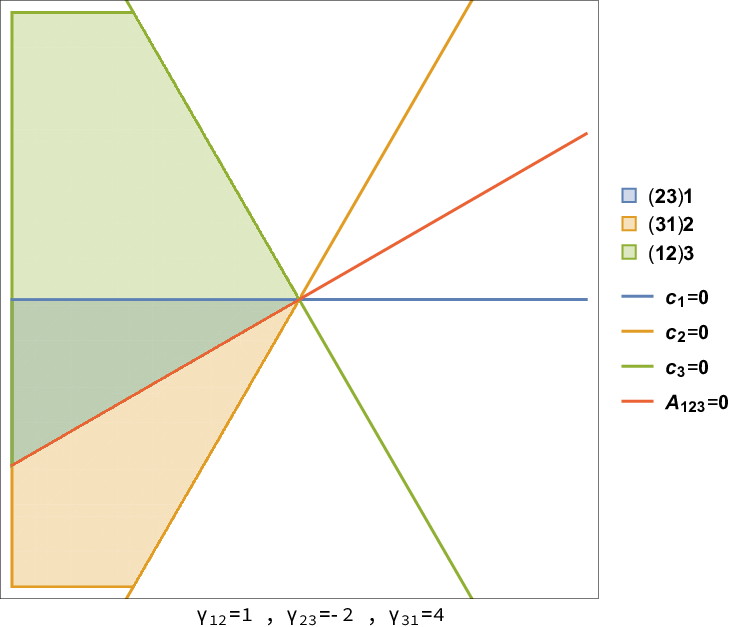
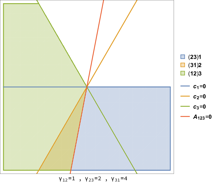
It is straightforward to check the consistency of the representation (2.34) with the primitive wall-crossing formula (2.24). For example, on the wall of marginal stability where vanishes we have and, as noted above (2.31), , and all have the same phase, so (2.33) reduces to
| (2.36) |
Using this in (2.32), the discontinuity of is then proportional to
| (2.37) |
consistently with the primitive wall-crossing formula (2.24).
On the other hand, it appears that (2.34) is discontinuous on the codimension one locus where the sign of changes, which does not coincide with any wall of marginal stability. However, due to the cyclic symmetry of , the discontinuity arises simultaneously for the flow tree and its images under cyclic permutations (see Fig. 4 for a plot of the stability regions of the various trees for two representative examples). As a result, while each of these contributions is discontinuous across , the sum over flow trees turns out to be smooth. Indeed, the coefficient of in (2.34) is the product of the ’s times
| (2.38) |
The key property ensuring the vanishing of this expression is the identity (valid for any )
| (2.39) |
Using it, one finds that (2.38) reduces to
| (2.40) |
Rewriting (2.33) as , it is now clear that this expression vanishes on the locus . Thus, after summing all trees, the total index is smooth across this locus and does not have any discontinuities beyond those predicted by wall crossing.
Given the fact that the discontinuity at cancels, one may wonder whether it is possible to rewrite the index in a form which does not involve at all, but only corresponding to the decay . To this end, let us rewrite the tree index (2.35) as
| (2.41) |
where we used the identity (2.39) to drop the term proportional to . Next, we use the same identity to replace
| (2.42) |
and relabel the charges after this replacement, arriving at
| (2.43) |
Finally, taking into account that and using the sign identity (A.1), one obtains that the tree index takes the form
| (2.44) |
This representation involves sign functions whose arguments are all expressed through the moduli at infinity and vanish only on the walls of marginal stability corresponding to the bound states of total charge .
2.6 Discrete attractor flow
As mentioned in §2.4, it appears that in order to compute the weight factor (2.23) ensuring the stability condition, one needs to solve the attractor flow along each edge in order to determine the explicit values of the moduli attached to each vertex. However, the weight factor (2.23) only depends on the moduli through the sign of evaluated at the parent vertex . We now explain how these signs can be determined in terms of asymptotic data without knowing itself, generalizing the procedure used above for .
The key property is again Eq. (2.13). Recalling the notation (2.26) and specializing to , it may be rewritten as
| (2.45) |
where are the coefficients (equal to 0 or 1) of the charge at the vertex on the basis spanned by the vectors assigned to the leaves, i.e. . This equation relates the coefficients , determining the stability of the BPS bound state , in terms of the coefficients , up to an irrelevant overall positive scale factor. While the relation (2.13) was derived in the context of a two-centered black hole with labelling the moduli at infinity, it holds just as well for nested sequences of two-centered bound states, where now labels the moduli at the parent vertex and the total charge should be replaced by . Thus, it allows to determine the coefficients at all vertices of the tree, starting from the root where and propagating them down the tree using the ‘discrete attractor flow’
| (2.46) |
at each vertex. Note that this relation is invariant under exchanging and , and ensures that . It is important however to keep in mind that the relation (2.46) assumes that the flow starting from can be continued all the way until it crosses the locus where (as opposed to terminating on a point where vanishes), and moreover that the central charges and are actually aligned at this point (as opposed to being anti-aligned).
For some purposes, it can be useful to have a formula expressing directly in terms of the moduli at spatial infinity, or more precisely in terms of the corresponding parameters . To this aim, let us consider a branch inside a flow tree, starting from the root and consisting of edges (see Fig. 5). We denote by the charges attached to the descendants of the vertices along the branch, such that it corresponds to the nested sequence of bound states
| (2.47) |
and . The charges () are in general linear combinations of the charges , () of the constituents attached to the leaves of the full tree, from which the branch has been extracted. We denote the moduli at the vertices along the tree by in the same order as charges, corresponding to the moduli at spatial infinity.

Our goal is to express the sign factor governing the stability of the innermost bound state in terms of . For this purpose, we define the following family of sign functions
| (2.48) |
where . The real parameters will be fixed momentarily in such a way that is related to its counterpart , in which the central charges are evaluated one step up along the attractor flow. To this end, we note that the discrete attractor flow equation (2.46) specialized for the vertex implies
| (2.49) |
where the proportionality coefficient is independent of and positive, and we defined
| (2.50) |
Since by definition is the point where the attractor flow crosses the wall of marginal stability , the central charges and have the same phase. Hence, one can replace the latter by the former in the left-hand side of (2.49), which then reproduces one term in the sum in (2.48). Thus, we find
| (2.51) |
where in the definition of on the right-hand side, we choose the first coefficients to be identical to the original ones, while the -th coefficient is related to the preceding ones by
| (2.52) |
The recursive relation (2.52) fixes all coefficients in terms of and . Moreover, due to , a shift of the initial conditions by results into an overall shift for all , which does not affect the ’s. Therefore, we can choose . Then (2.52) leads to
| (2.53) |
More generally, we find
| (2.54) |
for all . Using these relations, we can finally evaluate the relevant sign, which determines the stability of the innermost bound state in terms of ,1515 15 Note that, upon multiplying by the largest denominator , the argument of the sign becomes a homogenous polynomial of degree in the ’s.
| (2.55) |
Since the charges are linear combinations of the charges attached to the leaves of the full tree from which the branch is extracted, the argument of the sign can be written as a linear combination , where are defined in (2.26), and form a -dimensional real vector associated to the vertex and constructed out of the coefficients found above. In terms of these vectors, the weight factor (2.23) is rewritten as
| (2.56) |
which only depends on the asymptotic moduli through the variables defined in (2.26). This result gives a straightforward, algorithmic way of evaluating the tree index (2.22) in terms of asymptotic data without having to integrate the flow along each edge, provided such a flow exists. Furthermore, it shows that the tree index only depends on the charges through the DSZ matrix and on the moduli through the vector . The fact that the factor comes multiplied by in the definition (2.22) also shows that the tree index is a continuous function of for generic values of the ’s, justifying the prescription given in footnote 11 for dealing with the case of non-generic DSZ matrix.
Using the result (2.56), in appendix B we show that the tree index is also continuous across the ‘fake walls’ associated to the stability of intermediate bound states, despite the fact that contributions of distinct flow trees may jump on these loci. This is done with help of certain ‘flow vectors’ constructed from the coefficients . The recursive relation (2.52) allows to prove various symmetry properties of these vectors, which in turn reduce the proof of cancellation of the fake discontinuities to the cyclic property (2.39) of -factors. We defer this proof to the appendix because in the next subsection we shall provide a new representation for the BPS index which is manifestly smooth across all fake walls.
2.7 New formulae for the tree index
We have seen at the end of subsection 2.5 that for , it was possible to rewrite the tree index in such way that it was manifestly constant away from the physical walls of marginal stability corresponding to splittings of the total charge into . It is natural to expect that this should also be possible for any number of centers. Unfortunately, it is not straightforward to extend the tricks used for , due to the weights appearing explicitly in (2.22). While this can be done with some effort for , this procedure becomes extremely cumbersome.
To overcome this problem, we shall first rewrite the tree index in a form which does not contain the -factors anymore and is expressed in terms of another, -independent ‘partial index’. This form was inspired by the representation (4.4) of the Coulomb index, which will be the subject of section 4.
Proposition 1.
The tree index defined in (2.22) can be decomposed as
| (2.57) |
where runs over all permutations of and the ‘partial tree index’ is defined by1616 16 The subscript on is redundant since it equals the cardinality of the set . Nevertheless, we find it useful to display it and instead sometimes omit the arguments, the set of vectors and moduli .
| (2.58) |
where the sum runs over the set of planar flow trees with leaves carrying ordered charges .
Note that it is crucial to consider the refined index at for getting the representation (2.57), since each term in the sum over permutations is singular at . Nevertheless, the sum must be smooth in this limit, since the tree index (unlike the Coulomb index ) is a symmetric Laurent polynomial.
Proof.
To see the origin of the representation (2.57), let us expand all factors in (2.20) using the definition of in (2.18). Then each of the flow trees produces, up to a factor of , a sum of monomials of the form where . For each assignment of , there exists a unique permutation such that . For a given permutation , all trees contributing a term proportional to are planar flow trees ordered with respect to , i.e. trees ending on ordered points which can be drawn on the upper half plane without crossings.1717 17 For any , the number of such planar trees is , where is the -th Catalan number ( for ). The Catalan numbers satisfy the recursion relation , so that corresponding to the obvious ways of constructing a planar tree with leaves by merging two planar trees with and leaves, respectively. As for the usual flow trees, they are labelled by charges, with the charges assigned to the end-points, and contribute the weight given in (2.23) or (2.56). ∎
Since planar trees with end-points may be generated by merging two planar trees with and leaves, with running from 1 to (see footnote 17), it is easy to see that the partial index satisfies the following iterative equation1818 18 Throughout this section we assume that the second condition in (2.14) is automatically satisfied for the range of moduli of interest.
| (2.59) |
where we defined
| (2.60) |
while is the value of the moduli where the attractor flow crosses the wall for the decay . According to (2.46), this value corresponds to the parameters
| (2.61) |
While Eq. (2.59) allows for a very efficient evaluation of , it is also the starting point for obtaining new representations for the partial index which satisfy the properties stated at the beginning of this subsection.
To formulate our results, let us define the following quantities
| (2.62) |
and their specialization at , which we denote by
| (2.63) |
For all these objects are understood to be equal to one. For we have the vanishing property . In terms of these notations one can give two iterative representations for the partial index:
Proposition 2.
The partial tree index satisfies the following two recursion relations
| (2.64) |
where the sum runs over ordered partitions of , with largest size in the first relation, or in the second.1919 19 The restriction in the sum in the second line can be relaxed to . The stronger inequality is then automatically fulfilled due to . For , where is the number of parts, we defined
| (2.65) |
Note that the two representations differ only by a redistribution of the function : in the first one it contributes only to the sum over splittings of the set of charges into subsets, where in particular it arises as a factor in the last product, whereas in the second its effect is incorporated by the terms proportional to in (2.63). The two representations may be useful for different purposes. For instance, the second representation is suitable for the proof of convergence of the BPS partition function, whereas the first representation is more convenient for analyzing its modular properties [41], this is why we give here both of them. Since their proofs are essentially identical, we only present the proof for the first representation.
Proof.
Our proof will be inductive. It starts from in which case the formula (2.64) coincides with the definition of (see (C.3)). Let us now assume that it holds up to . Our aim is to show that the iterative equation (2.59) reduces to (2.64). Defining , we find that
| (2.66) |
Substituting (2.64) and (2.62) into the r.h.s. of (2.59) and denoting the second term in (2.64) by , one therefore gets
| (2.67) |
where we have used the sign identity (A.7). In the first contribution we immediately recognize the difference , whereas in the second contribution all terms can be combined into one sum over splittings by adding the condition . Denote the index for which this happens by . Then this contribution reads
| (2.68) |
Here we interchanged the two sums which allows to drop the condition , but adds the requirement (following from in the previous representation). In square brackets one recognizes the r.h.s. of (2.59) with replaced by . Hence, it is subject to the induction hypothesis which allows to replace this expression by and shows that (2.68) is equal to where the second term is due to the condition in the sum over splittings. Combining the two contributions, one finds which is exactly the first line in the required formula (2.64). The proof of the second line is similar using instead the sign identity (A.5). ∎
It is easy to verify the consistency of the representation (2.64) with the primitive wall-crossing formula (2.24). Since this essentially amounts to performing the manipulations used in the above proof in reverse, we shall omit this check, which is at any rate guaranteed by the previous results. On the other hand, for convenience of the reader, we have collected in appendix C.1 the explicit expressions for the partial indices in the form (2.64) up to . These expressions have been also checked by a direct recombination of signs in the original definition (2.58).
The representation (2.64) solves the problems about the sum over attractor flow trees formulated in section 2.4. However, it raises a new question: how can one extract the value of the tree index at ? Since by construction is a Laurent polynomial in , the limit is smooth, and therefore can be obtained by applying l’Hôpital’s rule to Eq. (2.57), i.e. acting on the numerator and on the denominator by before setting . This amounts to replacing the factor inside the sum by . Although this answers the question in principle, it may be desirable to have an alternative representation of the refined tree index where the monomials in are all combined into products of -factors. For , the result (2.44) provides such a representation. Ater recognizing the expression in the square brackets as the partial tree index in (C.4), it is natural to conjecture the following simple formula for any ,
Conjecture 1.
We have checked this conjecture by hand for and on Mathematica for higher . Since already the case is quite involved, we do not provide here these computations.
3 Attractor flows and quivers
In this section, we apply the flow tree formula to the context of quiver quantum mechanics, which describes the interactions of a set of mutually non-local BPS dyons in gauge theories or string theories with supersymmetry in four dimensions [22]. Using the well-known relation between the Higgs branch of this system and the moduli space of stable quiver representations, we obtain a formula which expresses the Poincaré polynomial of this moduli space, for arbitrary values of the stability conditions, in terms of Poincaré polynomials of quiver moduli space with lower dimension vectors evaluated at their respective attractor points.
3.1 A brief review of quiver quantum mechanics

Quiver quantum mechanics is a special class of 0+1 dimensional gauge theories with four supercharges [22]. Its field content is encoded in a antisymmetric integer matrix and a vector of positive integers known as the dimension vector. The model then includes vector multiplets for the gauge group and chiral multiplets transforming in the bifundamental representation if , or its complex conjugate if (note that we do not allow loops from any node to itself). We shall denote the bosonic component of these chiral multiplets by , where , , . The field content is conveniently represented by a quiver, i.e. a set of nodes associated to the gauge groups, and arrows going from node to node if , or in the opposite direction if . The antisymmetric matrix is the adjacency matrix of the graph formed by the nodes and arrows (see Fig. 6). When the quiver has oriented loops, the Lagrangian depends on a superpotential , which is a sum of -invariant monomials in the chiral multiplets . In addition, the Lagrangian depends on a real vector , whose entries are known as the Fayet-Iliopoulos (FI) parameters and associated to the center in each gauge group . For the purpose of counting BPS states, the overall scale of the ’s is irrelevant, so this vector can be viewed as a point in real projective space .
This supersymmetric quantum mechanics describes the interactions of a set of mutually non-local BPS dyons consisting of dyons of charge , dyons of charge , etc., upon identifying , and fixing the FI parameters as
| (3.1) |
where . Note that for an Abelian quiver (), this coincides with the definition of in (2.26). The superpotential (in case the quiver has oriented loops) may have a complicated dependence on the moduli, and we shall assume that it is generic in the sense that the Hessian at the critical points has maximal rank. Moreover, we stress that the quiver description is only valid in a region where the central charges are nearly aligned [5].
It will be convenient to introduce the -dimensional charge lattice spanned by the basis vectors , and the cone spanned by linear combinations with non-negative integer coefficients (and not vanishing simultaneously). Note that admits a natural partial order, if for all . For any charge vector , we denote . For the special case of the dimension vector , it follows from (3.1) that . Since the only dependence on the moduli arises through , we shall often use the symbol to denote the vector of FI parameters, without necessarily implying that they originate from a central charge function via (3.1).
Semi-classically, the quiver quantum mechanics admits two branches of supersymmetric vacua:
- •
the Higgs branch, where the gauge symmetry is broken to the center by the vevs of the chiral multiplet scalars ; the supersymmetric vacua are in one-to-one correspondence with the set of stable orbits of the action of the complexified gauge group restricted to the critical locus of the superpotential , where the stability condition is determined by the FI parameters. The set of supersymmetric vacua thus coincides with the moduli space of stable quiver representations widely studied in mathematics (see e.g. [44, 45] for entry points in the vast literature on this subject).
- •
the Coulomb branch, where the gauge symmetry is broken to and all chiral multiplets as well as off-diagonal vector multiplets are massive; the space of supersymmetric vacua is then isomorphic to the phase space which governs multi-centered BPS solutions in supergravity, where and indicates copies of the vector .
Quantum mechanically, BPS states on the Higgs branch are harmonic forms on the moduli space of quiver representations [22], while BPS states on the Coulomb branch are harmonic spinors on [42]. The group associated to physical rotations in acts on the cohomology of the Higgs branch via the Lefschetz action generated by contraction and wedge product with the Kähler form, while it acts on the cohomology of the Coulomb branch by lifting the Hamiltonian action of (2.7) on .
For the reasons explained below, the BPS index of interest in this set-up is the refined index of the BPS states on the Higgs branch. Mathematically, it is defined as the Poincaré polynomial of the moduli space of quiver representations with dimension vector and stability conditions , rescaled by a factor where is the complex dimension of :
| (3.2) |
Here, are the topological Betti numbers2020 20 It is also possible to define a two-variable polynomial which keeps track of the Hodge numbers and reduces to (3.2) at , and to the -genus at [27, §2.3]. Here we set for simplicity, but the flow tree formula has an immediate generalization to . of and stands for the set of FI parameters . In the case where the dimension vector is primitive and the superpotential is generic, is compact, so is a symmetric Laurent polynomial in , which can be viewed as the character of the Lefschetz action of on the moduli space . When is not primitive, is no longer compact, but one can still define the Poincaré polynomial using intersection cohomology. In that case, we define the rational invariant in the same way as in (2.15).
The simplest example is the Kronecker quiver, with two nodes of rank 1 and arrows from the first node to the second. The Higgs branch is either empty when , or given by the complex projective space . Its Poincaré polynomial is given by the same formula (2.17) which was arrived at by quantizing the Coulomb branch with . This coincidence between the cohomology of the Coulomb and Higgs branches is in fact a general property of quivers without oriented loops [20], and reflects the fact that the support of the BPS wave functions shifts from the Higgs branch to the Coulomb branch as the string coupling is increased [22]. For quivers with loops, the Coulomb branch is in general non-compact so the corresponding index is ill-defined. In contrast, the Higgs branch is compact for a generic choice of superpotential , at least for a primitive dimension vector. This is why we focus on the BPS index on this branch.
3.2 Flow tree formula for quivers
Since quiver quantum mechanics describes the dynamics of black hole bound states, it is natural to expect that the flow tree formula also applies in this context, and allows to express the total rational index in terms of sums of monomials in moduli-independent indices associated to all decompositions where the ’s lie in the positive cone . In order to formulate it however, we need to define the notions of ‘attractor flow’ and ‘attractor point’ in the context of quivers.
The first notion is obvious from the discussion in §2.6: the discrete attractor flow (2.46) only involves the parameters and the DSZ products associated to the constituents . In our setup they can be evaluated in terms of the coefficients of on the basis associated to the nodes of the quiver as
| (3.3) |
Note that these quantities define an auxiliary Abelian quiver with nodes associated to the constituents in the decomposition . From this data, one can then compute the tree index by constructing all stable attractor flow trees with leaves. The latter are rooted unordered binary trees , whose vertices are decorated by charge vectors with , such that the root carries charge , the leaves carry charges , and the charges add up at each vertex, . For a given decoration, we assign stability parameters at each vertex, equal to in (3.3) at the root and satisfying the ‘discrete attractor flow’ relation (2.46) along each edge,2121 21 Note that (2.46) assumed that the central charges were aligned on the walls of marginal stability, as opposed to being anti-aligned, but this assumption is automatically satisfied in the regime of validity of quiver quantum mechanics.
| (3.4) |
The tree index is then obtained via (cf. (2.20), (2.22), (2.23))2222 22 While only depends on vector through the DSZ matrix and parameters , for clarity we denote its arguments by .
| (3.5) |
where we recall that is defined in (2.18). In practice, it is easiest to generate the trees recursively, and discard those which do not satisfy the stability condition at one vertex without exploring further splittings. Alternatively, one may wish to use the representation (2.57) of as a sum of ‘partial tree indices’ defined by a sum over planar trees (see (2.58)), or the recursion formulae (2.59) and (2.64) of the previous section (see also (2.69) for a conjectural relation which does not require taking ).
As for the notion of attractor point, we observe that for a given dimension vector , the FI parameters defined by
| (3.6) |
are such that for any decomposition , the sign of is always opposite to the sign of , mimicking the property (2.9) of the supergravity attractor point [26]. Moreover, (3.6) automatically satisfies the condition , and is mapped to zero by the discrete attractor flow, as expected since a single-centered black hole should be described by a single node quiver. It is therefore natural to identify the attractor index with the Poincaré polynomial (3.2) evaluated for the charge vector and stability parameter . Of course, the attractor point can be defined in the same way for any vector , whether or not it coincides with the dimension vector of the original quiver.
With these identifications, we can now state the flow tree formula for quiver moduli in a mathematically precise way:
Conjecture 2.
For a -node quiver with adjacency matrix , dimension vector , stability parameters and generic superpotential , the rescaled Poincaré polynomial (3.2) of the quiver moduli space is given by (cf. (2.15))
| (3.7) |
where is the Moebius function and (cf. (2.21))
| (3.8) |
Here, the sum runs over all distinct unordered splittings of into sums of vectors with non-negative entries, is the order of the subgroup of the permutation group preserving the ordered set , is the ‘tree index’ defined using (3.3), and are the rational ‘attractor indices’, i.e. the same quantities as in (3.7) but evaluated for the dimension vector and stability parameters .
This conjecture is easily proven for Abelian quivers, i.e. when all . Indeed, (3.8) gives the correct value at the attractor point, since for vanishes by construction at that point, and it also satisfies the primitive wall-crossing formula, as shown in §2.4. In order to prove that (3.8) also holds for non-Abelian quivers, one would have to prove that it satisfies the general Kontsevich–Soibelman wall-crossing formula [2]. Unfortunately, we do not yet have a general proof of that fact.
For non-Abelian quivers without loops, however, we shall show in section 4.2 that the tree index coincides with the Coulomb index , so that the attractor indices coincide with the single-centered indices , and the flow tree formula becomes equivalent to the Coulomb branch formula reviewed in the next section. Since the latter has been shown [20] to be equivalent to Reineke’s formula [46] for non-Abelian quivers without loops, it follows that (3.8) also holds in this case. In particular, it must be consistent with the general wall-crossing formula.
For the most general case of non-Abelian quivers with loops, we do not have a direct proof that (3.8) is consistent with the general wall-crossing formula, but it is physically clear that the validity of the latter can only depend on general factorization properties of the tree index, and so should not be sensitive to the existence of loops (indeed, loops are responsible for existence of scaling solutions, but those are insensitive to wall-crossing). Hence we believe that the conjecture is true also in this general case, although this argument falls short of being a mathematical proof.
Alternatively, it may be possible to derive the flow tree formula from the Joyce-Song formula [3, 4], which relates the BPS indices and in arbitrary distinct chambers. Applying this formula for , we obtain a sum of products of with , all evaluated at the point . One can then repeat this process and express each of the ’s in terms of BPS indices at their respective attractor points . Since the charge of the constituents is always less than that of the total charge, this process terminates after a finite number of steps. It is interesting to note that the Joyce-Song formula also involves a sum over rooted decorated trees, albeit of a somewhat different type.
4 Comparing attractor and single-centered indices
In this final section, we compare the flow tree formula (2.21), expressing the total index in terms of attractor indices , with the Coulomb branch formula which expresses the same index in terms of single-centered indices . In §4.1, we briefly recall the statement of the Coulomb branch formula and the definition of the ‘Coulomb index’ which plays a central rôle in it. In §4.2 we show that the latter coincides with the tree index for charge configurations which do not allow scaling solutions, and conclude that for quivers without oriented loops. In the case where scaling solutions are allowed, corresponding to quivers with oriented loops, and in general differ, and so do and . While we do not yet know how to relate them explicitly in general, in §4.3 we work out their relation in the special cases of 3-centered and 4-centered configurations.
4.1 Review of the Coulomb branch formula
The Coulomb branch formula conjecturally expresses the total rational index defined in (2.15) in terms of single-centered indices as follows:
In both (4.1) and (4.2) the sums run over unordered decompositions of into sums of positive vectors or with . The functions are determined recursively by the so called “minimal modification hypothesis” (see [20, 28] for details) and their role is to ensure that the full refined index is a symmetric Laurent polynomial in . The function , known as the Coulomb index, is the only quantity on the r.h.s. of (4.1) which depends on the moduli . It is defined as the equivariant index of the Dirac operator on , computed by localization with respect to rotations around a fixed axis. The fixed points of the action of on are collinear solutions to the equations (2.6), classified by the order of the centers along the axis. Equivalently, they are critical points of the potential2323 23 It is worth noting that at the attractor point (3.6), the potential (4.3) becomes a sum of pairwise interactions, with , which is attractive for and repulsive for .
| (4.3) |
The sum over fixed points may be represented as a sum over all permutations of ,
| (4.4) |
where the ‘partial Coulomb index’ counts the critical points for a fixed ordering along the axis, weighted by the sign of the Hessian of after removing the trivial translational zero-mode. Under the reversal symmetry , picks up a sign , so that (4.4) is invariant under .
While the computation of the one-dimensional solutions to (2.6) becomes quickly impractical as increases, it was shown in [20] that the partial tree index can be efficiently evaluated by first rescaling by unless , and then dialing from (where only nearest neighbor interactions are kept) to (the configuration of interest).2424 24 This prescription assumes that the initial matrix is generic, in the sense explained in footnote 11 on page 11. For non-generic cases, one should first perturb the ’s such that they become generic, apply the previous prescription and then take the limit where the relevant ’s become zero. The value of the individual partial Coulomb indices may depend on the choice of deformation, but after summing over all permutations, the limit is independent of that choice [20]. The value at turns out to coincide with the function already introduced in (2.62).2525 25 In order to match this result with [20, (2.9)], observe that , where is the Heaviside step function, and are non-zero real numbers. Similarly, to make contact between (4.6) below and [20, (2.32)], note that and necessarily have the same sign whenever . In the absence of scaling solutions (or for quivers without loops), one can show that no jumps occur as increases from 0 to 1, so that is still given by its value at ,
| (4.5) |
In the presence of scaling solutions, the partial Coulomb index may jump several times as the deformation parameter is varied from 0 to 1. These jumps occur whenever the parameter is such that for some subset of , corresponding to all consecutive centers in colliding at one point. is then given by a sum over all possible jumps,
| (4.6) |
where are charge vectors with deformed inner product , and is the Coulomb index for colliding solutions. The latter vanishes for and satisfies its own recursion relation (see [20, §2.3.2]), initialized with the result for ,
| (4.7) |
Using this procedure, we can compute the Coulomb index for an arbitrary collection of non-zero vectors and generic stability parameters (collectively denoted by ). When the charges are such that no scaling solution is allowed, the result is the equivariant Dirac index of the compact phase space [18, 43], and is therefore a symmetric Laurent polynomial in with integer coefficients. In the presence of scaling solutions however, the phase space is non-compact and the above definition of produces instead a rational function of . While it might in principle be possible to construct a compactification of and incorporate additional fixed points from boundary components in order to produce a Laurent polynomial in , the Coulomb branch formula uses the rational function as defined above, but requires adjusting the functions in such a way that the full index obtained via (4.1) is a symmetric Laurent polynomial, provided the single-centered indices are. The minimal modification hypothesis of [20] gives a unique prescription for computing , based on the assumption that the missing contributions from the boundary of carry the minimal possible angular momentum. Note that this prescription does not take into account the condition of absence of closed timelike curves, which is presumably irrelevant in the context of quiver quantum mechanics, but needs to be checked by hand in more general cases (see e.g. [18, §3.2] for an example where this condition makes an important difference).
It follows from the results in [8] that the formula (4.1) is consistent with the general wall-crossing formula of [2, 3]. In cases where none of the decompositions allow for scaling solutions, relevant for quivers with no loops, all the factors in (4.2) vanish, so the Coulomb branch formula reduces to
| (4.8) |
which closely resembles (2.16). Indeed, we shall see in §4.2 than in this simplified case, the single-centered indices agree with the attractor indices .
A different simplification occurs when is primitive and such that all charge vectors appearing in each decomposition are distinct and primitive. In this case, relevant for Abelian quivers, the Coulomb branch formula (4.1) simplifies to
| (4.9) |
In this case, the rational functions are fixed by demanding that the coefficient of the monomial in be a Laurent polynomial in . Requiring that are invariant under and vanish at fixes them uniquely [18]. The reason why (4.9) differs from (2.16) is that the attractor indices include contributions both from single-centered black holes and scaling solutions.
4.2 Quivers without loops
In this subsection, we shall show that for quivers without loops, such that no scaling solutions are allowed, the tree index and Coulomb index coincide for any set of charges and moduli. This will turn out to imply that the attractor and single-centered indices, and , also coincide for all .
In order to show the equality , the main observation is that the corresponding partial indices and are locally constant functions of the parameters whose only discontinuities lie on the walls of marginal stability where , where they both jump according to the primitive wall-crossing formula. Therefore, it suffices to show that they coincide at one value of the .
A convenient choice is to take the attractor point (3.6) which in our case is . It is an immediate consequence of the iterative equation (2.59) that at this point the partial tree index vanishes. On the other hand, the partial Coulomb index (4.5) reduces to the function defined in (2.63). We shall now show that this function vanishes whenever is the adjacency matrix of a generic -node quiver without loops. The result for non-generic matrices then follows by continuity.
First, note that there exists different choices of signs for (out of ) such that the quiver has no oriented loops, and all those choices are related by permutations (indeed, any generic quiver defines a total order on ). For each of these choices of signs, there exists a unique source and sink . Consider the restricted quiver obtained by keeping only nearest neighbor interactions. The restricted quiver has a set of sources and sinks which lie either at the endpoints , , or at the points where changes sign. Obviously, and . Now, assume that was non-zero. This means that for each in , the sign of is the same as the sign of . Thus, whenever changes sign, so does . The key observation is the following: whenever and have opposite sign, then the sign of is opposite to the sign of , which is equal to . Thus, if is a sink of the restricted quiver distinct from the endpoints, i.e. , , then , hence , which shows that cannot be a sink of the full quiver. Similarly, if is a source of the restricted quiver distinct from the endpoints, then it cannot be a source of the full quiver. Thus, the source and sink of the full quiver must be the endpoints. But again, cannot be the source nor the sink, since and have the same sign. Similarly, cannot be the source nor the sink. Thus, we have reached a contradiction with the hypothesis that was non-zero. Therefore, the partial Coulomb index at the attractor point vanishes for any generic quiver without oriented loops. As a result, we conclude that , and therefore . Since both and are continuous functions of (for generic, fixed values of ), this equality continues to hold even if is not generic.
Having established that , we can now apply the Coulomb branch formula (4.8) for equal to . Since (and therefore ) vanishes at that point whenever , it immediately follows that for any dimension vector. The flow tree formula (2.21) is therefore equivalent to the Coulomb branch formula (4.8), which is known to agree with Reineke’s formula for quivers without loops provided whenever is one of the basis vectors and zero otherwise [20]. We conclude that the flow tree formula holds for quivers without loops.
4.3 Abelian quivers with loops
Let us now allow for loops in the quiver diagram, and hence for the presence of scaling solutions, restricting to the Abelian case. This corresponds to the inclusion of the second term in the partial Coulomb index (4.6) and, given the results of the previous subsection, of the second term in the second representation of the partial tree index given in (2.64). Besides, we have to take into account the contributions to the BPS index generated by the functions and captured by the formula (4.9). Unfortunately, we have not yet been able to find general relation between the attractor and single-centered indices following from equating the two expansions. Below we provide explicit results for two particular cases: and .
4.3.1 Three centers
For , the partial tree index can be found in (C.4), whereas the partial Coulomb index is given in (C.6). In the latter formula, the term in the first line is the result for a quiver with nearest-neighbor interactions, while the second line arises from contributions of scaling solutions when the parameter is changed from to . It is easy to check that the second line vanishes unless all have the same sign (so that the quiver has an oriented loop) and satisfy , in which case it equals . The latter condition implies that satisfy the triangular inequalities (so that scaling solutions are allowed), the restriction that be the largest of all three being due to the special choice of ordering.
The matching of the first terms in (C.4) and (C.6) is just the statement (4.5). The second terms are however different. Using the sign identity (A.1) repeatedly, one can rewrite the difference between the two partial indices as
| (4.10) |
which is moduli-independent and vanishes unless all have the same sign and satisfy . The moduli-independence is a consequence of the fact that and have the same discontinuities across the walls of marginal stability and . Because vanishes at the attractor point, the conditions for non-vanishing of the difference are, of course, the same which ensure the non-vanishing of itself.
The difference between the Coulomb and tree indices, and , can be obtained by summing (4.10) over permutations. If, for example, , which is a configuration allowing scaling solutions, then the difference reads
| (4.11) |
Note that in this case is a rational function with a double pole at , while is always a symmetric Laurent polynomial in .
We can now relate the single-centered invariant to the attractor index . For this purpose, we compare the Coulomb branch formula (4.9) with (2.21) for . Using the fact that for basis vectors, for sums of two basis vectors, and for any pairs of vectors , we conclude that
| (4.12) |
Applying the minimal modification hypothesis to determine [20], for the case considered in (4.11) we arrive at
| (4.13) |
where is the parity (0 or 1) of . By construction, the difference is a symmetric Laurent polynomial.
4.3.2 Four centers
For , the two partial indices are given in (C.5) and (C.10). While the first terms in each expression coincide, the remaining terms are quite different, and the moduli-dependence does not cancel in their difference . This is in fact consistent with the structure of the two expansions of the BPS index. Indeed, comparing (4.9) and (2.21) and taking into account (4.12), one finds
| (4.14) |
Thus, the moduli-dependence of the difference of the two indices at must be non-trivial, so as to cancel the moduli-dependence in the second line. To check that this is indeed the case, note that the relation (4.14) can be rewritten as
| (4.15) |
where
| (4.16) |
Evaluating this combination using in particular (4.10), one arrives at
| (4.17) | |||||
As expected, the result is moduli-independent, as required for the consistency of (4.15). Moreover, vanishes if is the adjacency matrix of a generic quiver without loops. Unfortunately, the result (4.17) does not immediately suggest a generalization to .
Acknowledgments.
The authors are grateful to Jan Manschot for collaboration at an initial stage of this project, and to Sibasish Banerjee, Frederik Denef, Greg Moore and Ashoke Sen for discussions. The hospitality and financial support of the Theoretical Physics Department of CERN, where this work was initiated, is also gratefully acknowledged.Appendix A Sign identities
In this appendix we collect several sign identities which are used in the main text. The basic identity, which is used in most manipulations, is
| (A.1) |
Its validity follows from that its two sides are locally constant functions with the same discontinuities and having the same value for, say, positive .
Next, let us prove the following identity2626 26 If , the r.h.s. can be rewritten as .
| (A.2) |
We proceed by induction. For it trivially holds. Assuming that it holds for , we find the smallest and order the variables so that this is . This allows to write
| (A.3) | |||||
where at the second step we have used the induction hypothesis.
The identity (A.2) can be used to derive another one. Let us choose in (A.2) to run from 0 to and take . Then the identity gives
| (A.4) |
Taking the sum of this new relation with (A.2) and rearranging the terms, one then obtains
| (A.5) |
Finally, a useful particular case of the above identities is obtained by setting . In this way, one finds
| (A.6) | |||||
| (A.7) |
where is the parity of , i.e. it equals 1 if is odd and 0 if is even.
Appendix B Flow vectors and cancellation of fake discontinuities
Given the results of section 2.6, it is natural to attach to each vertex on the flow tree a -dimensional vector
| (B.1) |
where is the depth of the vertex and the coefficients are constructed from charges , attached to the branch of the tree joining the vertex with the root (see Fig. 5), as in (2.54). The arguments of the sign functions appearing in the stability conditions will then reduce to inner products of with the ‘central charge vector’ where (cf. (2.26)). However, this construction must be slightly modified in order to take into account that the coefficients are defined only up to an overall shift. Moreover, it is useful to allow for a non-trivial metric on , depending on the physical context,2727 27 For instance, for the D4-D2-D0 brane system on a Calabi-Yau threefold, the relevant metric is where are the triple intersection numbers, is the D4-component of the electromagnetic charge , and are the Kähler moduli of the Calabi-Yau. so that the inner product takes the form . The results presented here are completely independent of this metric, so for the purposes of the present analysis we could take .
Thus, we define the flow vector assigned to a vertex as the projection of on the hyperplane orthogonal to the unity vector ,
| (B.2) |
or in terms of components
| (B.3) |
where and . We also modify the definition of the central charge vector taking its components to be
| (B.4) |
It is then easy to see that by virtue of we have
| (B.5) |
i.e. the flow vectors correctly encode the moduli dependent signs entering in (2.23).
Note that if one of the charges, say , can be decomposed into a sum (for instance, can be the charges assigned to the leaves of the tree), then the above construction has a natural embedding into . To display it, let us introduce two operations: embedding and contraction. For arbitrary vectors and , they are defined by and where
| (B.6) |
and have also obvious extension to matrices. Then, if we require that and take the -dimensional central charge vector to be defined as above with the set of charges replaced by , it is easy to check that the vector satisfies . Thus, both constructions are equally suitable for describing the stability conditions of the flow tree.
This freedom allows to avoid the inconvenience of working with vectors of different size. To this end, it is sufficient to expand all charges in the basis of charges assigned to the leaves of the tree and embed all vectors into using the above prescription. In practice, however, this is not necessary. In this appendix we will work simultaneously with at most two vectors when we define their mutual orthogonal projections. In such case the relevant branch is shown in Fig. 7 and in the notations of the picture it is enough to embed the vectors corresponding to vertices and in the minimal common space . Moreover, if (i.e. belongs to the branch connecting with the root), only one of the vectors requires the embedding. Below we always choose the flow vectors in the minimal possible representation and drop the dimension label.

The flow vectors turn out to be very handy for showing the cancellation of discontinuities across ‘fake walls’ in the sum over flow trees. Moreover, very similar vectors play a crucial role in the study of convergence and modular properties of indefinite theta series defining the BPS partition function for D4-D2-D0 black holes [47, 48, 41]. Before turning to the first of these topics however, we state some important properties satisfied by the flow vectors, referring to subsection B.1 for the proofs.
Proposition 3.
If is not the root vertex, the vector has the form
| (B.7) |
where is the set of vertices on the path from towards the root (including the root), and is a vector which is cyclically symmetric in , and (assuming that belongs to the left branch of , i.e. that ).
Next, let us introduce the projection of on the subspace orthogonal to
| (B.8) |
Such projections naturally appear when one evaluates the discontinuities of BPS indices across walls determined by equations . It turns out that the projections also possess certain symmetry properties summarized in the following proposition:
Proposition 4.
Depending on the relative position of vertices and on the tree, one has four different situations:
- 1.
If is the root vertex of an attractor flow tree and belongs to its left branch, then coincides with which is constructed for the tree obtained from by removing the root and its right branch. Equivalently,
(B.9) i.e. the attractor flow is undone by one step and the central charges are evaluated at the moduli corresponding to the parent to parent vertex.
- 2.
If is not the root vertex and is either ancestor of , or a child of one of its ancestors, then is the same for the three trees shown in Fig. 8.

Figure 8: Three attractor flow trees relevant for the case 2 of the Proposition. Here the circles denote the branches of the flow tree attached to the corresponding vertices, whereas the dots indicate that there can be any number of vertices with the corresponding branches. - 3.
If is a descendant of , then
(B.10) where has the same symmetry as , i.e. it is cyclically symmetric in , and .
- 4.
If the pair does not correspond to any of the previous cases, i.e. a path from to goes at least 2 steps up and some steps down, then is cyclically symmetric in , and .
The first part of Proposition 4 immediately allows to see the consistency of the attractor flows with the primitive wall-crossing formula (2.24). Indeed, the discontinuity of the weight (2.56) due to the sign factor arising at the root vertex evaluates to
| (B.11) |
where and are the two branches of the tree growing from the root vertex and we defined
| (B.12) |
for a subtree not containing . Here we indicated explicitly with an upper index that the vector is defined for the tree . But due to Proposition 4 (case 1), for it coincides with the vector defined for either or so that . Thus, one obtains
| (B.13) |
After multiplying by , by the product of the attractor indices , and summing over all trees, this is indeed in agreement with the primitive wall crossing formula.

While only the first part of Proposition 4 entered this proof, the remaining three parts ensure the cancelation of the fake discontinuities appearing due to the sign factors in (2.23) attached to non-root vertices. To see this, note that due to Proposition 3, the same fake wall arises for three different trees whose parts containing vertex are shown in Fig. 9. They are obtained by cyclic permutations of the subtrees , and . Their discontinuities at the fake wall are given by
| (B.14) |
where the factors have been defined in (B.12), is the part of not shown in Fig. 9, and the last factor comes from (B.7). Case 2 of the Proposition 4 ensures that the factors are the same for all three choices of , whereas cases 3 and 4 tell us the same about
| (B.15) |
Finally, one finds that
| (B.16) |
where the factor in the square brackets is the same for all trees shown in Fig. 9. Thus, only the first two -factors in (B.16) differ the three discontinuities. It remains to note that in the notations of Fig. 9, for the first tree, and , whereas for other trees they are given by cyclic permutations. Then the cancellation of fake discontinuities follows from the identity (2.39).
B.1 Proof of the symmetry properties of the flow vectors
Now we fill the gap and prove the symmetry properties of the flow vectors and their orthogonal projections stated above. We concentrate only on the relevant branch of the tree and label the charges as in Fig. 7. The flow vectors are constructed from the coefficients (2.54) as explained in the beginning of this section. These coefficients satisfy an important symmetry property under permutations of , which will be the starting point of our analysis.
Lemma 1.
Under a permutation of , the coefficients transform as
| (B.17) |
where is the parity of the permutation.
Proof.
Let us use the freedom of shifting all by the same constant and define
| (B.18) |
where, as usual, . Then
| (B.19) |
are permuted under permutations of with the sign given by , while are invariant up to the same sign, as can be shown inductively from the recursion
| (B.20) |
and the fact that is invariant under cyclic permutations of whenever . Returning to the original coefficients , we arrive at the transformation (B.17). ∎
Using this Lemma, it is straightforward to prove Proposition 3.
Proof of Proposition 3:
In this case it is sufficient to consider only the branch of the tree connecting vertex to the root. Our aim is to prove that is mapped by a cyclic permutation to .2828 28 We multiply the argument of the sign by only, whereas in (B.7) the factor is extracted. But for depend on the first three charges only in the combination and therefore are cyclically symmetric in these charges. Thus, they are irrelevant for the present discussion. This can be done using the explicit expression (B.3) for the components of the vector and Lemma 1. Indeed, the transformation law (B.17) implies (for a cyclic permutation )
| (B.21) |
which is the required statement. ∎
In the following we will also need the coefficients of , which is, in the notations of Fig. 5, the flow vector assigned to vertex and embedded into , the habitat of the flow vector for . From (B.6) it follows that
| (B.22) |
where the coefficients are obtained by the following substitution
| (B.23) |
Note that under this substitution, for . For , only such appear in the expression for (2.54). Then one has the following
Lemma 2.
Under a permutation of , the coefficients transform as
| (B.24) |
where
| (B.25) |
Proof.
The check of the transformation for is straightforward. For we use the recursive formula
| (B.26) |
Proceeding by induction and noticing that the sum in (B.26) can be extended to start from , one obtains
| (B.27) |
where we changed the summation variable and used the property as well as the two recursion relations (2.52), (B.26). ∎
These shifted coefficients are useful, in particular, to make explicit the properties of under the exchange of and for . Indeed, whereas for , are independent of these charges, for we can write
| (B.28) |
where are defined by the recursion relation (cf. (2.52))
| (B.29) |
It is immediate to see that
| (B.30) |
where
| (B.31) |
whereas , defined by
| (B.32) |
are invariant under the exchange of and .
Let us also introduce
| (B.33) |
Using (B.28), one finds
| (B.34) |
Furthermore, using (B.30), one obtains
| (B.35) |
Lemma 3.
Under the exchange of and , the coefficients transform as
| (B.36) |
Proof.
Now we are ready to prove Proposition 4.
Proof of case 1:
If is the root vertex, the components of and embedded into are given by
| (B.37) |
| (B.38) |
where and we label the charges as in Fig. 5 with and . One finds for these vectors
| (B.39) |
| (B.40) |
This implies
| (B.41) |
This is precisely the vector corresponding to the tree obtained by removing the root. This proves the first statement of the Proposition. ∎
Proof of case 2:
Labeling the charges as in Fig. 8, the components of the vectors and , corresponding to the first tree and embedded into , can be found in (B.38) and (B.22), respectively. For these vectors, one obtains
| (B.42) |
| (B.43) |
This implies
| (B.44) |
where is defined in (B.33).
First, to show the equality of for the first two trees, we need to show that the vector (B.44) is invariant under the exchange of and . Using that under this exchange transform as in (B.17) where one should replace by and by , whereas the transformation of is given by Lemma 3 (see (B.36)), it is immediate to see that
| (B.45) |
For the third tree, we need to consider the embedding . The components of such vector are given by
| (B.46) |
where
| (B.47) |
On the other hand, the vector , due to Proposition 3, coincides up to a factor, which anyway cancels in the orthogonal projection, with . Thus, now
| (B.48) |
where
| (B.49) |
Let us find the coefficients explicitly. First, we have
| (B.50) |
Note, in particular, the following property
| (B.51) |
where the quantity on the r.h.s. was defined in (B.31). Next, we have (cf. (B.28))
| (B.52) |
where the tilde means the same substitution as in (B.47). In particular, one has
| (B.53) | |||||
The resulting recursive relation coincides with (B.32), which allows to conclude that
| (B.54) |
Furthermore, using the linearity of in (which follows from the linearity of in ), it is easy to see that
| (B.55) |
The last term can be evaluated using Lemma 2, which gives
| (B.56) |
As a result, one obtains
| (B.57) |
Substituting this into the definition (B.49), it is straightforward to verify that the result coincides with (B.34) and (B.35), i.e.
| (B.58) |
Then comparing (B.48) and (B.44), one concludes that the vectors describing orthogonal projections for the two trees indeed coincide,
| (B.59) |
This completes the proof of the second statement of the Proposition. ∎
Proof of case 3:
In this case, if is not a child of , the statement is trivial. Indeed, in this case depends on , and only through the sum of these charges so that it is automatically cyclically symmetric. Furthermore, by Proposition 3, is also cyclically symmetric up to an overall factor, but this factor cancels in the orthogonal projection . This allows to conclude that is cyclically symmetric, and since also depends only on the sum of the permuted charges, the statement follows.
Thus, it remains to analyze the case when is a child of . Let us label the charges as in Fig. 5 with and so that the components of the vectors and are given by
| (B.60) |
where the coefficients are defined in (B.23). For these vectors, one obtains
| (B.61) |
| (B.62) |
This implies
| (B.63) |
Applying the transformations (B.17) and (B.24) for a cyclic permutation (), one finds
| (B.64) | |||||
where the last term vanishes due to symmetrization in . This result proves the third statement of the Proposition. ∎
Proof of case 4:
The proof in this case is analogous to the previous one for the case when was not a child of . Indeed, in the present case again depends on , and only through their sum, whereas is cyclically symmetric by Proposition 3 up to a factor which is canceled in the projection. Thus, is indeed cyclically symmetric. ∎
Appendix C Explicit expressions for partial indices
In this appendix we provide explicit expressions for the partial tree and Coulomb indices up to . The results are conveniently formulated in terms of
| (C.1) |
C.1 Tree index
C.2 Coulomb index
The partial Coulomb index coincides with (C.3), whereas the result for follows from (4.6) and is given by [20, (2.57)]
| (C.6) |
The expression for is already much more complicated. It is found to be [20, (2.61)]
| (C.7) | |||||
and is determined by the function [20, (2.59)]
| (C.8) |
evaluated at if , and if , where the parameters are given by2929 29 The necessary condition that is ensured by the fact that a rational number lies in iff (in which case and ) and by non-vanishing of the sign factors in (C.7) multiplying the sign dependent on given .
| (C.9) |
Substituting into (C.7) and applying repeatedly the sign identity (A.1), one can show that
| (C.10) | |||||
References
- [1] B. Pioline, “Four ways across the wall,” J.Phys.Conf.Ser. 346 (2012) 012017, 1103.0261.
- [2] M. Kontsevich and Y. Soibelman, “Stability structures, motivic Donaldson-Thomas invariants and cluster transformations,” 0811.2435.
- [3] D. Joyce and Y. Song, “A theory of generalized Donaldson-Thomas invariants,” American Mathematical Soc., 2012, 0810.5645.
- [4] D. Joyce, “Generalized Donaldson-Thomas invariants,” 0910.0105.
- [5] F. Denef and G. W. Moore, “Split states, entropy enigmas, holes and halos,” JHEP 1111 (2011) 129, hep-th/0702146.
- [6] D. Gaiotto, G. W. Moore, and A. Neitzke, “Four-dimensional wall-crossing via three-dimensional field theory,” Commun.Math.Phys. 299 (2010) 163–224, 0807.4723.
- [7] E. Andriyash, F. Denef, D. L. Jafferis, and G. W. Moore, “Wall-crossing from supersymmetric galaxies,” JHEP 1201 (2012) 115, 1008.0030.
- [8] J. Manschot, B. Pioline, and A. Sen, “Wall Crossing from Boltzmann Black Hole Halos,” JHEP 1107 (2011) 059, 1011.1258.
- [9] E. Diaconescu and G. W. Moore, “Crossing the wall: Branes versus bundles,” Adv. Theor. Math. Phys. 14 (2010), no. 6, 1621–1650, 0706.3193.
- [10] T. Dimofte and S. Gukov, “Refined, Motivic, and Quantum,” Lett. Math. Phys. 91 (2010) 1, 0904.1420.
- [11] D. Gaiotto, G. W. Moore, and A. Neitzke, “Framed BPS States,” Adv. Theor. Math. Phys. 17 (2013), no. 2, 241–397, 1006.0146.
- [12] F. Denef, “Supergravity flows and D-brane stability,” JHEP 0008 (2000) 050, hep-th/0005049.
- [13] B. Bates and F. Denef, “Exact solutions for supersymmetric stationary black hole composites,” JHEP 11 (2011) 127, hep-th/0304094.
- [14] S. Ferrara, R. Kallosh, and A. Strominger, “ extremal black holes,” Phys. Rev. D52 (1995) 5412–5416, hep-th/9508072.
- [15] F. Denef, B. R. Greene, and M. Raugas, “Split attractor flows and the spectrum of BPS D-branes on the quintic,” JHEP 05 (2001) 012, hep-th/0101135.
- [16] E. Andriyash, F. Denef, D. L. Jafferis, and G. W. Moore, “Bound state transformation walls,” JHEP 1203 (2012) 007, 1008.3555.
- [17] J. Manschot, “Wall-crossing of D4-branes using flow trees,” Adv.Theor.Math.Phys. 15 (2011) 1–42, 1003.1570.
- [18] J. Manschot, B. Pioline, and A. Sen, “A Fixed point formula for the index of multi-centered N=2 black holes,” JHEP 1105 (2011) 057, 1103.1887.
- [19] A. Collinucci and T. Wyder, “The Elliptic genus from split flows and Donaldson-Thomas invariants,” JHEP 05 (2010) 081, 0810.4301.
- [20] J. Manschot, B. Pioline, and A. Sen, “On the Coulomb and Higgs branch formulae for multi-centered black holes and quiver invariants,” JHEP 05 (2013) 166, 1302.5498.
- [21] A. Chowdhury, S. Lal, A. Saha, and A. Sen, “Black Hole Bound State Metamorphosis,” JHEP 1305 (2013) 020, 1210.4385.
- [22] F. Denef, “Quantum quivers and Hall/hole halos,” JHEP 10 (2002) 023, hep-th/0206072.
- [23] K. Hori, H. Kim, and P. Yi, “Witten Index and Wall Crossing,” JHEP 01 (2015) 124, 1407.2567.
- [24] C. Cordova and S.-H. Shao, “An Index Formula for Supersymmetric Quantum Mechanics,” 1406.7853.
- [25] C. Hwang, J. Kim, S. Kim, and J. Park, “General instanton counting and 5d SCFT,” JHEP 07 (2015) 063, 1406.6793. [Addendum: JHEP04,094(2016)].
- [26] J. Manschot, B. Pioline, and A. Sen, unpublished (2013).
- [27] J. Manschot, B. Pioline, and A. Sen, “From Black Holes to Quivers,” JHEP 1211 (2012) 023, 1207.2230.
- [28] J. Manschot, B. Pioline, and A. Sen, “The Coulomb Branch Formula for Quiver Moduli Spaces,” Confluentes Mathematici 2 (2017) 49–69, 1404.7154.
- [29] I. Bena, M. Berkooz, J. de Boer, S. El-Showk, and D. Van den Bleeken, “Scaling BPS Solutions and pure-Higgs States,” JHEP 1211 (2012) 171, 1205.5023.
- [30] A. Sen, “Entropy Function and AdS(2) / CFT(1) Correspondence,” JHEP 0811 (2008) 075, 0805.0095.
- [31] A. Sen, “Arithmetic of Quantum Entropy Function,” JHEP 08 (2009) 068, 0903.1477.
- [32] A. Dabholkar, J. Gomes, S. Murthy, and A. Sen, “Supersymmetric Index from Black Hole Entropy,” JHEP 1104 (2011) 034, 1009.3226.
- [33] S.-J. Lee, Z.-L. Wang, and P. Yi, “Quiver Invariants from Intrinsic Higgs States,” JHEP 1207 (2012) 169, 1205.6511.
- [34] S.-J. Lee, Z.-L. Wang, and P. Yi, “BPS States, Refined Indices, and Quiver Invariants,” JHEP 1210 (2012) 094, 1207.0821.
- [35] J. M. Maldacena, A. Strominger, and E. Witten, “Black hole entropy in M-theory,” JHEP 12 (1997) 002, hep-th/9711053.
- [36] J. Manschot, “Stability and duality in N=2 supergravity,” Commun.Math.Phys. 299 (2010) 651–676, 0906.1767.
- [37] E. Andriyash and G. W. Moore, “Ample D4-D2-D0 Decay,” 0806.4960.
- [38] J. de Boer, F. Denef, S. El-Showk, I. Messamah, and D. Van den Bleeken, “Black hole bound states in ,” JHEP 0811 (2008) 050, 0802.2257.
- [39] S. Alexandrov, J. Manschot, and B. Pioline, “D3-instantons, Mock Theta Series and Twistors,” JHEP 1304 (2013) 002, 1207.1109.
- [40] S. Alexandrov, S. Banerjee, J. Manschot, and B. Pioline, “Multiple D3-instantons and mock modular forms I,” Commun. Math. Phys. 353 (2017), no. 1, 379–411, 1605.05945.
- [41] S. Alexandrov and B. Pioline, “Black holes, instantons and mock modular forms”, 1808.08479, to appear in Commun. Math. Phys. (2019).
- [42] J. de Boer, S. El-Showk, I. Messamah, and D. Van den Bleeken, “Quantizing N=2 Multicenter Solutions,” JHEP 05 (2009) 002, 0807.4556.
- [43] H. Kim, J. Park, Z. Wang, and P. Yi, “Ab Initio Wall-Crossing,” JHEP 1109 (2011) 079, 1107.0723.
- [44] H. Derksen and J. Weyman, “Quiver representations,” Notices of the AMS 52 (2005), no. 2, 200–206.
- [45] M. Reineke, “Moduli of representations of quivers,” Proceedings of ICRA XII, Toruń, Poland, August 15-24, 2007, 0802.2147.
- [46] M. Reineke, “The Harder-Narasimhan system in quantum groups and cohomology of quiver moduli.,” Invent. Math. 152 (2003), no. 2, 349–368.
- [47] S. Alexandrov, S. Banerjee, J. Manschot, and B. Pioline, “Indefinite theta series and generalized error functions,” Selecta Mathematica 24 (2018) 3927–3972, 1606.05495.
- [48] S. Alexandrov, S. Banerjee, J. Manschot, and B. Pioline, “Multiple D3-instantons and mock modular forms II,” Commun. Math. Phys. 359 (2018), no. 1, 297–346, 1702.05497.