Unconditional Stability for Multistep ImEx Schemes: Practice
Abstract
This paper focuses on the question of how unconditional stability can be achieved via multistep ImEx schemes, in practice problems where both the implicit and explicit terms are allowed to be stiff. For a class of new ImEx multistep schemes that involve a free parameter, strategies are presented on how to choose the ImEx splitting and the time stepping parameter, so that unconditional stability is achieved under the smallest approximation errors. These strategies are based on recently developed stability concepts, which also provide novel insights into the limitations of existing semi-implicit backward differentiation formulas (SBDF). For instance, the new strategies enable higher order time stepping that is not otherwise possible with SBDF. With specific applications in nonlinear diffusion problems and incompressible channel flows, it is demonstrated how the unconditional stability property can be leveraged to efficiently solve stiff nonlinear or nonlocal problems without the need to solve nonlinear or nonlocal problems implicitly.
Keywords: Linear Multistep ImEx, Unconditional stability, ImEx Stability, High order time stepping.
AMS Subject Classifications: 65L04, 65L06, 65L07, 65M12.
1 Introduction
This paper builds on the theoretical work [53] on the unconditional stability of linear multistep methods (LMMs). While [53] introduced a new unconditional stability theory for implicit–explicit (ImEx) methods, and presented a novel class of ImEx LMMs that involve a stability parameter, this paper develops strategies on how to select the time stepping parameter and the ImEx splitting in an optimal fashion. The key focus is on problems for which an ImEx splitting is warranted in which both the implicit and the explicit terms are stiff, for example because the stiff terms are difficult to treat implicitly.
Conventional ImEx splittings often treat all stiff terms implicitly to ensure that one does not encounter a stiff time step restriction (one usually accepts a time step restriction from the non-stiff explicit part). However, as demonstrated in [53], this is not always required: one may treat stiff terms explicitly and nevertheless avoid a stiff time step restriction, provided the implicit term and the scheme are properly chosen. This paper provides strategies on how to make these choices (splitting and scheme) in practical problems. We do so through the use of the unconditional stability theory from [53], which is based on geometric diagrams that play a role analogous to the absolute stability diagram in conventional ordinary differential equation (ODE) stability theory. Specifically, we present strategies on how to achieve unconditional stability via (i) choosing the splitting for a given scheme; (ii) modifying a time-stepping scheme for a given splitting; and (iii) designing the splitting and the scheme in a coupled fashion. In addition, we employ the stability theory to provide new insights on the limitations of popular semi-implicit backward differentiation formulas (SBDF). In fact, we show that the new ImEx LMMs generalize SBDF methods, in a way that they overcome some of their fundamental stability limitations.
1.1 Problem setting
We are concerned with the time-evolution of linear ODEs of the form
| (1.1) |
Here , , and is an external forcing. We assume that gives rise to asymptotically stable solutions — i.e. solutions to the homogeneous ODE decay in time (the eigenvalues of are in the strict left-half-plane). This assumption can be relaxed; however then additional caveats are required (see §6 for when has a zero eigenvalue, or §8 for when has purely imaginary eigenvalues).
For the right hand side , an ImEx splitting is conducted [7, 18, 60, 34], i.e. is split into two parts, , where is treated implicitly (Im) and is treated explicitly (Ex). Clearly, the splitting is non-unique, and in fact, any matrix defines a splitting by choosing . For this ImEx splitting, we now require the time-stepping scheme to be unconditionally stable. This is a stringent, but very practical property (especially when is stiff) as it allows one to choose a time step as large as accuracy requirements permit.
Note that the theory in this paper is developed for linear ODEs, as this assumption allows for a rigorous geometric stability theory involving unconditional stability diagrams. However, we then extend the results, in an ad-hoc but rather natural fashion, to nonlinear problems as well.
1.2 Examples from partial differential equations
A crucial source of stiff problems is the method-of-lines (MOL) semi-discretization of a partial differential equation (PDE). In that situation, rather than having one single right hand side , one faces a family (with the mesh size) that approximates a spatial differential operator . A key property of the time-stepping strategies studied here is that for many PDE problems, the choice of ImEx splitting and scheme can in fact be conduced on the level of differential operators, or equivalently, to hold for the family , uniformly in (see Sections 6 and 7).
An important PDE situation in which unconditional stability is important is the MOL discretization of diffusion. A fully explicit treatment of diffusion gives rise to a stiff time step restriction . Hence, for problems in which diffusion represents the highest spatial derivative, a common approach is to include all of the discretization of into the implicit part , and leave as the remaining non-stiff terms. Such an approach will then avoid a stiff time step restriction. However, treating all stiff terms of implicitly may in general be costly (see §6); and in fact it is not always necessary. Having new approaches that allow one to treat (some of the) stiff terms explicitly, without incurring a stiff time step restriction, can be a significant practical benefit. In problems where is stiff and costly to treat fully implicitly, this opens the door for designing a well-chosen ImEx splitting where contains only part of the stiff components of , and is much more efficient to treat implicitly.
1.3 Background and relation to other works
ImEx unconditional stability has been studied in numerous theoretical and practical works. On the theoretical side, general abstract sufficient conditions for unconditional stability and arbitrary multistep schemes are stated in [2, 3, 4, 5]. Although these conditions have the advantage of incorporating nonlinear terms (i.e. is allowed to be a nonlinear operator), they have the drawback that they require the implicit matrix be larger (in the sense of an appropriate norm) than , and are overly restrictive for the problems we consider (e.g. they do not apply to Example 2).
Generally speaking, in the context of multistep methods, proofs for unconditional stability are commonplace for first and second order methods. Meanwhile, for higher order schemes, unconditional stability is usually only studied numerically, and in limited settings. This gap is likely due to the limitations that existing high-order methods encounter (see §5). Important works in which unconditional stability is proved for first or second order methods, or numerically observed in higher order schemes, are the following papers (and references therein). Some of the first applications involving unconditional stability originated in the 1970s, with alternating direction implicit (ADI) methods [19]. Others include magneto-hydrodynamics [30]; unconditional stability (also referred to as unconditionally energy stable, or as convex-concave splitting methods) for phase-field models [23, 9, 22, 54, 57, 25, 26, 61, 22, 8]; applications to fluid-interface problems [21]; incompressible Navier-Stokes equations [39, 48, 31, 41, 43, 49]; Stokes-Darcy systems [45], compressible Navier-Stokes equations [10, 11], and PDEs with the explicit treatment of non-local terms [6, 59]. One disadvantage of low (i.e. first or second) order methods is that they can also have large error constants for dissipative PDEs [16] and dispersive PDEs [15], thus further reducing their applicability for the long-time numerical simulations. We differ from these previous works in several ways:
- 1.
We include higher order schemes as part of the study.
- 2.
Whereas many existing works use von-Neumann analysis or energy estimates that are tailored to a specific problem, we make use of recently introduced unconditional stability diagrams [53]. The diagram approach simplifies the design of high-order unconditionally stable schemes and is applicable to a wider range of applications.
- 3.
We include variable ImEx time stepping coefficients. It may be surprising that stability considerations for ImEx schemes do not require all stiff terms to be included in . In fact, ImEx schemes can even go far beyond such a restriction: not only can be stiff, it can (in some sense) even be larger than , while still retaining unconditional stability. The underlying mechanism is that is chosen in a way that stabilizes the numerical instabilities created by the explicit treatment of with a suitable (simultaneous) choice of a splitting and time stepping scheme.
It should also be stressed that there are numerous time stepping approaches (not strictly multistep methods) for specific application areas that possess good stability properties. Recently, high order unconditional stable methods for ADI applications have been obtained by combining second order multistep schemes with Richardson extrapolation [12, 13, 14]. For PDE systems that have a gradient flow structure, new conditions [55] allow for the design of third order, unconditionally energy-stable Runge-Kutta (RK) methods. Other techniques include: semi-implicit deferred correction methods [51]; semi-implicit matrix exponential schemes where the linear terms are treated with an integrating factor [42, 40, 50]; and explicit RK schemes with very large stability regions for parabolic problems [1].
1.4 Outline of this paper
This paper is organized as follows. After introducing the key notation and definitions (§2), a self-contained review of the employed unconditional stability theory is provided that takes a different viewpoint than [53] by placing a practical emphasis on the eigenvalues of , . Section 4 and onward (including A) contain new results. Section 4 provides recipes for designing (optimal) unconditionally stable ImEx schemes that minimize the numerical error. Section 5 characterizes the limitations of the well-known SBDF methods. Section 6 uses insight from §5 to overcome the limitations of SBDF and devise optimal high order (i.e. beyond 2nd order) unconditionally stable schemes for the variable-coefficient and non-linear diffusion problems. This section includes new formulas for ImEx splittings and schemes (accompanied by rigorous proofs in A); as well as computational examples. Section 7 studies an application example that is motivated by incompressible Navier-Stokes flow in a channel and provides general insight into stability issues in computational fluid dynamics. Section 8 provides an outlook and conclusions, and B lists the specific ImEx coefficients to be used in practice.
2 Introduction to the ImEx schemes and unconditional stability property
This section introduces the assumptions, notations, and ImEx schemes used throughout the paper. As discussed above, we are interested in unconditional stability for ImEx splittings of equation (1.1) where in general both the implicit matrix , and the explicit matrix are allowed to be stiff.
We restrict to splittings in which is Hermitian (symmetric in the real case) negative definite, i.e. has strictly negative eigenvalues:
| (2.1) |
Here we have adopted the standard notation on vectors (or ):
Note that itself is not assumed symmetric/Hermitian or negative definite. Furthermore, assumption (2.1) on is not overly restrictive, because for any given one can choose symmetric negative definite, and then set . Note that spectral methods (for the spatial discretization of PDEs) may give rise to a complex matrix , which is why we do not restrict to be real. It is also worth noting that much of the theory we present still persists even when is not Hermitian and negative definite (see Section 8).
Finally, we remark that the implicit treatment of a matrix in multistep methods (or even Runge-Kutta methods), requires one to solve linear systems with coefficient matrices of the form , where is a constant and is the time step. For symmetric negative definite, those system matrices are positive definite and thus favorable for fast solvers (chapter IV, lecture 38, [58]).
We will generally assume that the problem gives rise to a preferred/natural matrix structure (symmetric, negative definite) that one wishes to treat implicitly; however, its overall magnitude is up to choice. In other words, the user fixes and would accept any implicit matrix of the form (with the splitting parameter ), provided that such an yields unconditional stability. This is in a spirit similar to [19]. For example, in spatial discretizations of a variable coefficient diffusion PDE where , the user may prefer an implicit treatment of the constant coefficient Laplacian , however, would accept any constant multiple as well, i.e. . Writing where is fixed, introduces the scalar as a key parameter. This paper shows how to choose in a systematic fashion to obtain unconditionally stability.
We restrict our attention to ImEx versions of linear multistep methods (LMMs) [7, 18]; however it is worth noting that some of the concepts developed here may extend to other time stepping schemes as well, such as Runge-Kutta (multi-stage) ImEx schemes. The general form of an -step LMM applied to the ODE (1.1) with a splitting is:
| (2.2) |
Here is the time step, the variable (so that is explicit in (2.2)), is the numerical solution (with a slight abuse of notation) evaluated at the -th time step, and . We refer to the values , with as the ImEx (time stepping) coefficients. The LMMs of the form (2.2) require initial conditions . The computation of these initial conditions to sufficient accuracy is a separate problem (chapter 5.9.3, [47]), and is not considered here. When discussing stability it will be useful to define the polynomials , , , using the ImEx coefficients in (2.2):
| (2.3) |
Given the ImEx coefficients, one may write down the polynomials , , , or alternatively, given polynomials , , , one may read off the different coefficients in front of to obtain the time stepping coefficients .
In this work we utilize a one-parameter family of ImEx coefficients, introduced in [53], that have desirable unconditional stability properties. The new ImEx coefficients are characterized by a parameter , i.e. they are functions of a single ImEx parameter , and are defined for orders through . Formulas for the new coefficients , in terms of , may be found in Table 4; and substituting different values of into these formulas yields different ImEx schemes. For example, the new one-parameter ImEx schemes for first () and second order () take the form:
| (2.4) | ||||
| (2.5) | ||||
For brevity we have set in the formulas (2.4)–(2.5), however one may include it in the explicit term (or even the implicit term) as in equation (2.2). Although the formulas for the coefficients might appear unruly, they have simple polynomial expressions.
Remark 1.
(ImEx coefficients from Table 4 written in polynomial form) For orders , and , the ImEx coefficients , for from Table 4 correspond to the following polynomials:
| (2.6) | ||||
| (2.7) |
The relationships between the polynomials, i.e. , and as the -th order Taylor polynomial of ensure that the ImEx coefficients satisfy the order conditions required to define an -th order scheme.
Note that in the Remark 1, the polynomial has roots that approach as . This is not an accident, and it is this property that will eventually lead to good unconditional stability properties for the new schemes.
Equations (2.4)–(2.5), as well as the 3rd, 4th, 5th order schemes in Table 4, define families of time-stepping schemes. When the value is substituted into the coefficient formulas in equations (2.4)–(2.5), one obtains the well-known backward differentiation formulas for the coefficients of , also referred to as semi-implicit backward differentiation formulas (SBDFr, where denotes the order of the scheme):
Choosing values yields different (new) schemes. We have only displayed orders in the above expressions, however coefficients are also given for orders in Table 4. Lastly we note that the new ImEx schemes are zero-stable for any value , and the coefficients satisfy the order conditions [53] to guarantee that they define an -th order scheme (i.e. solving (2.2) using the coefficients approximates the solution to (1.1) with an error that scales like as ).
Each fixed set of ImEx coefficients, such as SBDF (), or ImEx versions of Crank-Nicolson, or even schemes not considered in this paper, provide unconditional stability for only a certain set of matrix splittings — and these may not include a practitioner’s desired splitting for a given problem. Introducing the one-parameter family of ImEx schemes (parameterized by ) provides the flexibility needed to attain unconditional stability for new classes of matrices beyond the capabilities of what is possible using a fixed set of coefficients. This point becomes particularly apparent in §5, in the discussion of the limitations of SBDF methods. This gain in unconditional stability offered by the parameter may come with a trade-off of increasing the numerical approximation error constants. Thus, an important discussion (see §4) is how to choose an ImEx scheme (i.e. how to choose ) for a given problem splitting (i.e. ) to balance the trade off of gaining unconditional stability while minimizing the numerical error. Or, even better, how to choose the splitting and scheme in a coupled fashion.
Our goal is to avoid unnecessarily small time step restrictions in the numerical scheme (2.2). To do this we examine when (2.2) is unconditionally stable — i.e. the numerical scheme (2.2) with remains stable regardless of how large one chooses the time step . Formally, we adopt the following definition:
Definition 2.1.
(Unconditional stability) A scheme (2.2) is unconditionally stable if: when , there exists a constant such that
Note that may depend on the matrices , , and the coefficients , but is independent of the time step , the time index , and the initial vectors , .
It is important to note that unconditional stability of an ImEx LMM like (2.2) can be difficult to determine in practice, as this question depends simultaneously on the choice of coefficients and the splitting . The purpose of introducing a new stability theory in [53] was to remedy this difficulty and formulate unconditional stability (or failure thereof) in terms of two separate computable quantities: one quantity that depends only on the coefficients , and one that depends only on the splitting . The theory then allows for a variety of possibilities:
- (i)
- (ii)
- (iii)
3 The unconditional stability theory
In this section we review the unconditional stability theory from [53] — which imposes conditions on and the time-stepping coefficients that (when satisfied) ensure the unconditional stability of (2.2). The stability theory will then provide a guide for choosing the ImEx coefficients and/or splitting that guarantee unconditional stability for a given problem (i.e. ). The unconditional stability theory is somewhat analogous to the classical absolute stability theory (chapter 7, [47]), as it relies on a stability diagram — and we highlight the parallels with an example here:
Example 1.
(Absolute stability theory) Given an ODE of the form , the absolute stability diagram is defined as
| (3.1) | ||||
The scheme (3.1) is stable with time step , if and only if every eigenvalue of (i.e. ) satisfies (with the possible exception of repeated eigenvalues , and time steps that lie on the boundary ).
A key feature of the absolute stability theory is that it decouples the stability criteria into (i) a property of the matrix only (i.e. the eigenvalues), in relation to (ii) a property of the time stepping scheme only (i.e. ). Decoupling the stability theory is extremely useful; for instance, it allows one to determine which matrices can be solved using a given time stepping scheme. The unconditional stability theory in this section will parallel that of the absolute stability theory, and:
- •
Introduce the unconditional stability diagram (defined solely by ); and provide formulas for the diagrams to the schemes corresponding to Table 4.
- •
Provide computable quantities in terms of that are analogous to the eigenvalues of in Example 1. Unconditional stability will then be framed in terms of the computable quantities lying inside the unconditional stability region.
3.1 The unconditional stability diagram
The absolute stability theory in Example 1 was obtained by replacing the matrix with one of its eigenvalues — resulting in a (simpler) stability analysis of a scalar ODE. In a similar spirit, if can be simultaneously diagonalized (for instance when they are commuting and diagonalizable matrices), then may be replaced by their eigenvalues — resulting likewise in a scalar ODE. The unconditional stability diagram can then be derived from this scalar ODE. We stress that although the diagram is derived here assuming are simultaneously diagonalizable, the diagram is also applicable to general matrices (i.e. that do not commute), as outlined below. Suppose is a simultaneous eigenvector to and and satisfies
| (3.2) |
Here (and real) since is symmetric/Hermitian and positive definite. Substituting into the ODE (1.1) yields the scalar equation
| (3.3) |
One can then examine stability for the ImEx scheme (2.2), applied to equation (3.3) (with the term treated implicitly and the term explicitly), in the usual way: set , to obtain a polynomial equation for the growth factors
| (3.4) |
Here are the polynomials defined in (2.3). Note that the polynomial equation (3.4) was used in [7] for the purpose of determining CFL-type time step stability restrictions for advection-diffusion problems; and also in [24] in the context of computing absolute stability-type diagrams for ImEx schemes (see also [44] for a treatment of delay differential equations). In both cases, the matrices were assumed to be simultaneously diagonalizable, and neither study was focused on unconditional stability. Equation (3.4) is also sometimes used as a (non-rigorous) model for stability in the case when are not simultaneously diagonalizable. The study of unconditional stability digresses from prior work by re-parameterizing equation (3.4) with the substitution and :
| (3.5) |
Note that takes on all values as varies between and ; and that . For a fixed mode, i.e. fixed and , unconditional stability demands that the growth factors solving equation (3.4) are stable for all . Viewed in the context of (3.5), this requirement leads to the definition of the unconditional stability diagram : the values for which the growth factors to (3.5) are stable for all (including )
Here we say that is stable if ; and for technical convenience we exclude (non-repeated) values of . Thus far, the definition for is very general and may be computed for any set of ImEx LMM coefficients . It is also crucial to note that is defined only in terms of the ImEx scheme coefficients.
It was proved (Thm. 8, Prop. 9 [53]) that for the schemes in Table 4, the value of (i.e. requiring stability for large time steps, ) imposes the most severe restriction on the growth factors in equation (3.5). This theoretical result has the consequence that the set is completely determined by setting in (3.5), leading to the simplification
| (3.6) |
We stress that (3.6) is not necessarily a general property of ImEx LMM — but it holds for the schemes in Table 4. Equation (3.6) is useful as it allows one to compute (Thm. 8 [53]) in terms of a boundary locus formulation (chapter 7.6, [47]) with the polynomials and introduced in Remark 1:
- (B1)
The set (for orders ) includes the origin (i.e. ) and has the boundary
(3.7) - (B2)
The right-most point and left-most point of are on the real axis with:
- (B3)
In the asymptotic limit , the set approaches the circle , where
Note that has a center at and radius ; and hence becomes arbitrarily large as . Therefore, becomes large as .
Figure 1 plots the stability diagrams for different orders and values — and also shows that asymptotically approaches (as ) the large circle . Having formulas for the shape and size of as functions of will be important for designing unconditionally stable schemes (2.2), and for characterizing the limitations of well-known schemes such as SBDF. Lastly, we note that the ImEx schemes parameterized by bare some similarity to the non-ImEx schemes with large regions of absolute stability originally examined in [35, 36]. However, we will eventually choose the parameter value to be as large as possible (to minimize the error), while maintaining unconditional stability. This is of a fundamentally different nature than the non-ImEx study carried out in [35, 36].

We now come to our first condition for unconditional stability — which is stated in terms of the generalized eigenvalues
| (3.8) |
Note that a negative sign was added, for convenience, in the definition of to make positive definite; and that is equivalent to the eigenvalues of .
Condition 1.
(Unconditional stability when are simultaneously diagonalizable) Given time stepping coefficients with diagram , and simultaneously diagonalizable matrices with generalized eigenvalues , we have the following…
-
Sufficient conditions: The scheme (2.2) is unconditionally stable if every generalized eigenvalue lies in , i.e. .
-
Necessary conditions: If a generalized eigenvalue is not in , i.e. , then the scheme (2.2) is not unconditionally stable.11 1 Strictly speaking, the precise theorem (Proposition 10, [53]) is that if , or where is the boundary locus of , then the scheme is not unconditionally stable. However, for practical purposes, the boundary locus can be ignored since it is a curve.
In Condition 1, the (NC) and (SC) are essentially identical and give a sharp characterization of unconditional stability. Although Condition 1 is useful when are simultaneously diagonalizable, we also wish to consider matrices and that do not commute. The results in [53] generalize the (SC) in Condition 1 to arbitrary matrices ( still symmetric positive definite) by replacing the set with a (somewhat larger) set defined in terms of a numerical range (also known as the field of values). Specifically, let be any real number (different values of will eventually be useful for different problem matrices ), and introduce the following sets:
| (3.9) |
The set can also be written, using a change of variables , as:
| (3.10) | ||||
| (3.11) |
Here is the definition of the numerical range of a matrix; and is a well-known set (chapter 1, [33]) that may be computed using a sequence of eigenvalue computations [37]. Note that depends only on the matrix splitting and is independent of the time stepping coefficients. Condition 1 may then be modified as follows.
Condition 2.
((Theorem 5, [53]) Unconditional stability for a general splitting )
Note that in Condition 2 the (NC) are the same as in Condition 1, however the (SC) are no long the same — due to the non-commuting matrices. In Conditions 1–2 the (SC) provide a target criterion that will ensure unconditional stability; while the (NC) will provide insight into when a scheme may fail to be unconditionally stable.
We provide a brief explanation here for why one should replace with the sets in Condition 2. If one seeks an eigenvector solution to (2.2) of the form ; and then multiplies equation (2.2) from the left by , then one obtains equation (3.5), with the modification that the value is no longer a generalized eigenvalue, but is given by a general Rayleigh quotient:
Hence, ensuring guarantees that the value of in (3.5) lies within the unconditional stability region.
Remark 2.
(Properties of the numerical range and ) Since the sets can be written in terms of a numerical range, they exhibit all the well-known properties of a numerical range. The numerical range for a matrix is convex (Hausdorf-Toeplitz theorem), bounded, and always contains the eigenvalues of , i.e. . In the case when is a normal matrix, is the convex hull of the eigenvalues. Hence, the convex hull of is contained in (for all ).
Remark 3.
Different values of may modify the size of in the complex plane. Condition 2 only requires one value of to satisfy (even if other values of violate ).
4 How to choose the ImEx parameter and splitting
In this section we provide general recipes for choosing the ImEx parameter and the matrix splitting for a problem matrix . The recipes are based on minimizing a proxy for the numerical error while ensuring that the sufficient conditions (SC) are satisfied.
Solely based on the formulas for , one could think that one should use ImEx coefficients with very large unconditional stability region , by taking . After all, such a choice would increase the chance of unconditional stability by ensuring that fits inside thereby satisfying the (SC) in Conditions 1–2.
However, choosing small without any regard for the error is not a good strategy. Specifically, there is a trade-off between schemes with good unconditional stability properties (i.e. small and large ) and the resulting numerical accuracy. Ideally, one would choose so that the scheme’s numerical approximation error is minimized, while still guaranteeing unconditional stability. However, because the true error is generally not accessible, we use as a proxy for the approximation quality, which is justified by the following remark.
Remark 4.
(Dependence of the global truncation error constant on ) The global truncation error (GTE) at time is defined by . Because the ImEx schemes in Remark 1 are formally of -th order, for any fixed , the GTE scales (for small) like . The error constant depends on , , , and the time stepping coefficients. Formulas for the behavior of the GTE error constants in a LMM may be computed in terms of the polynomials (see equation (2.3), p. 373, in [28]) and . In particular, one may compute two separate error constants. One error constant is obtained when the ImEx scheme is applied as a fully implicit scheme (i.e. , ) as . A second error constant may be computed when the ImEx scheme is applied to a fully explicit splitting (i.e. , ), where . In general, for a fixed splitting , one then has a GTE that scales like
| (4.1) |
A more detailed description, along with numerical error tests verifying the asymptotic formula (4.1) may be found in [53].
Remark 4 indicates that for a fixed splitting , the GTE error is (asymptotically) minimized by taking a maximum value of . Moreover, as a secondary trend, if a family of ImEx splittings is considered, then it is generally observed that smaller values of yield a smaller GTE. Hence, one should generally choose as large as possible and small, while still satisfying the (SC) constraint in Conditions 1–2.
We now provide recipes for three different scenarios that may arise in practice. Recipe 1 specifies how to choose the ImEx parameter to achieve unconditional stability when a fixed matrix splitting is specified (i.e. this a special case where and ).
Example 2.
(Simple example using the Recipe 1) Consider the ODE , with implicit part and explicit part (this ODE splitting was also examined in [53]), for which we wish to devise a 3rd order () unconditionally stable scheme. For this splitting, the matrices and are (trivially) simultaneously diagonalized with . Condition 1 then requires for both the (NC) and (SC). For a 3rd order scheme, , we use the formulas for and in (B2) so that the constraint reads:
| (4.2) |
The largest value that satisfies the inequality (4.2) (with replaced by ) is: . Any value will guarantee unconditional stability — i.e. one could take a fraction so that . Substituting this value into the formulas in Table 4 yields the ImEx coefficients.
In situations where one is using a pre-programmed ODE or black-box solver, it may not be possible to modify the time stepping coefficients . Instead, one may have the ability to modify the matrix splitting by varying the parameter . Recipe 2 outlines how one may choose the parameter when the scheme and the matrix are fixed. The recipe uses the sets and , whose dependence on is characterized by the following remark.
Remark 5.
(Dependence of and on ) The sets and are simple transformations of the -independent sets and :
| (4.3) |
Here the identities (4.3) follow from a direct calculation using :
| (4.4) | ||||
| (4.5) |
Due to properties (4.3), one can, for fixed and , pre-compute the sets and . The range and generalized eigenvalues are then simply rescaled versions (w.r.t. the point 1 in the complex plane) of the corresponding range and eigenvalues using and , where yields the scaling parameter. This becomes important in §5 when we examine and overcome the fundamental limitations of SBDF.
Section 5 provides examples that illustrate Recipe 2. Recipes 1 and 2 are in line with a common perspective on ImEx schemes. Either, one has to determine the ImEx parameter when the matrix splitting is fixed; or choose the splitting parameter when the scheme is fixed. In practice, there may be cases in which neither of these two approaches is able to achieve unconditionally stability.
We therefore advocate, whenever possible, to allow to simultaneously vary the ImEx parameter and the splitting parameter . It turns out that this yields an enormous amount of flexibility when designing unconditionally stable schemes. Many splittings of the form , where and are chosen and predetermined from the problem (see Sections 6–7 for specific PDE applications), can be stabilized this way.
4.1 Additional details for PDEs: choosing
When arises as the spatial discretization of a PDE with meshsize , one does not have a fixed matrix splitting , or , but rather a family of splittings parameterized by : , or . In this situation, it is crucial to be able to choose the parameters independent of the meshsize — i.e. to have one and the same ImEx scheme be unconditionally stable for an entire family of splittings , or . If, for example, unconditional stability required one to choose the ImEx parameter as a function of the grid size (i.e. such as ), then such a choice would have a deleterious effect on the GTE (GTE ), and limit the benefits of unconditional stability.
To be able to choose a single set of parameters that stabilizes the family of splittings for all , some care must be taken to ensure the matrix is properly chosen relative to . Once a suitable choice of is fixed, one may use the Recipe 3 to simultaneously choose for unconditional stability.
Remark 6.
(Guidelines for choosing when is the spatial discretization of a PDE) Generally speaking, it is a good idea to ensure that has the same derivative order as , as backed up by the following heuristic scaling argument. Suppose
A natural choice for might be
(one could include a variable coefficient approximation as well). Many spatial approximation methods yield the scaling , hence one may expect some of the eigenvalues of to scale like . The re-scaling formulas in Remark 5 then imply that there may be generalized eigenvalues that scale like . This gives rise to three cases for choosing :
- •
If , some of the generalized eigenvalues diverge as . Using formula (B3) for the asymptotic behavior of , the ImEx parameter would then have to scale like as (and fixed ) to ensure that these large eigenvalues remain inside (to satisfy the (NC)). Hence, cannot be chosen independent of the mesh .
- •
If , some of the generalized eigenvalues as (and fixed ). In this case, the formulas in (B2) show that only order schemes contain the point (see Figure 1). Hence, is generally not a good choice if one is looking for a scheme with orders .
- •
If , then all generalized eigenvalues have a chance (based solely on the scaling of ) to be uniformly bounded (i.e. do not become arbitrarily large) as ; and also remain strictly bounded away from as . In this case, there is a chance to obtain high order by means of choosing the parameters independent of .
5 Limitations of unconditional stability for SBDF schemes
In §3, the unconditional stability region was used to derive sufficient (SC) and necessary (NC) conditions for unconditional stability. Using these conditions, this section illustrates how the geometrical properties of can be used to understand the fundamental limitations that classical SBDF methods possess with regards to unconditional stability. Specifically, two significant qualitative transitions occur: (i) moving from 1st to 2nd order schemes for non-symmetric matrices ; and (ii) moving from 2nd to 3rd order for symmetric matrices . Guided by Recipe 2, we discuss under which circumstances a choice of exists so that a splitting is unconditionally stable with SBDF.
Case 1: non-symmetric. Let be a non-symmetric matrix that, together with , has both a range and eigenvalues with negative real part, i.e. they lie strictly in the left-half plane, but are not necessarily contained on the real line. Such a situation occurs for instance in discretizations of advection–diffusion PDEs (with an implicit diffusion, and explicit advection). The following transition arises between first and second order SBDF when the ImEx splitting is taken as :
- 1.
SBDF1 can always be made unconditionally stable, by choosing suitably large. This is due to the fact that for SBDF1 is a circle with its right-most point at . Hence one can always rescale (see Remark 5) so that .
- 2.
SBDF2 can, in general, not be made unconditionally stable by means of choosing . This is a result of the cusp at in (see Figure 2). If, for instance, the imaginary part of is larger (in absolute value) than its real part, then the scaled eigenvalue (see Remark 5) will never enter , regardless of the value of .
We highlight these insights with the following simple example.
Example 3.
(A non-symmetric ) Consider the following non-symmetric matrix and choice of matrix :
The generalized eigenvalues are , and is a triangle consisting of the convex hull22 2 The matrix is normal, which results in a simple expression for the range . of the eigenvalues. Note that, for simplicity, we have chosen an example in which and commute. Hence, Condition 1 may be used. We also plot to illustrate how to apply Condition 2 (which is stronger than Condition 1) when one is faced with matrices that do not commute. Figure 2 visualizes that SBDF1 can be made unconditionally stable with , while SBDF2 cannot be made unconditionally stable by only varying . However, high order schemes (i.e. ) that are unconditionally stable for (3) are possible by varying both , as seen in Figure 3.


Case 2: symmetric. Let be a symmetric negative definite matrix. Assume now that is such that the range of and eigenvalues are real and strictly negative. Such a situation arises for instance in the discretization of a purely parabolic (gradient flow) problem. The following transition occurs between second- and third-order schemes for the splittings :
- 1.
SBDF2 can always be made unconditionally stable, by choosing suitably large. This is due to the fact that the right-most point of for SBDF2 is , and is real and negative, so one can always rescale (see Remark 5) into .
- 2.
SBDF3 can, in general, not be made unconditionally stable by means of choosing . This is because the right-most point of is (instead of ), so that a negative real may be impossible to contain within via the choice of .
Unconditional stability limitations of SBDF, applied to splittings , may be overcome by simultaneously choosing , i.e. by following Recipe 3.
Example 4.
(A symmetric ) Consider the following symmetric matrices:
Then , and is an interval along the real axis. Figure 4 shows that SBDF2 can be made unconditionally stable with , while SBDF3 cannot be made unconditionally stable by only varying . In contrast, third to fifth order schemes that are unconditionally stable for (4) are possible by varying both , as seen in Figure 5.
6 Examples from diffusion PDEs
In this section we apply the unconditional stability theory from §4.1 and Recipe 3 to PDE diffusion problems with spatially varying, and even non-linear diffusion coefficients. The presented methodology highlights how one can avoid a stiff time step restriction (here: of diffusive type , where is the smallest grid size) — or any time step restriction for that matter — while inverting only simple constant coefficient matrices. This allows one to leverage fast solvers where an implicit treatment of (i.e. using the fast Fourier transform) can be carried out much more rapidly than a fully implicit treatment of (i.e. that contains all the stiff diffusive terms). The new ImEx coefficients (see §5) enable high order time stepping beyond what is possible using only SBDF methods.
6.1 Numerical discretization
We start by providing numerical details for the one-dimensional Fourier spectral methods used. Computations in three dimensions are then conducted by naturally extending the one-dimensional approach via Cartesian products. We use a periodic computational domain ; discretize space using a uniform grid with an even number of grid points ; and approximate the function at by , where:
Because our analysis is based on the matrices that are written in terms of Fourier transforms, it is useful to introduce notation for the discrete Fourier transform (DFT) matrix , and for the spectral differentation matrix — even though in practice one will never use those matrices, but rather use the fast Fourier transform (FFT) to compute . The DFT matrix has the coefficients:
The (spectral) differentiation of a function defined on the uniform grid amounts to a scalar multiplication in Fourier space, i.e. . Hence, the matrix takes the form: , where denotes the matrix with diagonal entries of the vector:
Since , the matrix is skew-Hermitian and the matrix is Hermitian. If is diagonalized by , then solving for in the implicit step of the evolution (2.2), i.e. , is done via two FFTs.
6.2 An FFT-based treatment for the variable coefficient diffusion equation
We now devise unconditionally stable ImEx schemes for the variable coefficient diffusion equation (with diffusion coefficient )
| (6.4) |
that make use of an FFT-based treatment of the implicit matrix . The choice of splitting is guided by §4.1, and the choice of parameters by Recipe 3. To ensure a high spatial accuracy, we adopt a spectral discretization of equation (6.4) and set:
Note that is a dense matrix and (due to the -dependence of ) is not diagonalized via the DFT matrix . To seek an ImEx splitting of , we follow the guidelines in Remark 6: the matrix has two factors of and hence the implicit matrix should have two factors of as well. This motivates the following matrix splitting:
| (6.5) |
i.e. and .
Our goal is to determine, following Recipe 3, the parameters that guarantee unconditional stability. Before doing so, we must discuss a caveat: the matrices and are not invertible — which was an assumption in the derivation of the conditions for unconditional stability. We do not provide a general treatment for when is not invertible due to subtleties that may arise (for instance when the null space of interacts with through the ImEx evolution). However, for the specific splitting (6.5), the unconditional stability theory presented in §3 (and recipes in §4) can be applied with only a minor adaptation, namely: the definition/computation of the sets and are done on the subspace where is invertible, as follows.
The matrix has a null space spanned by the constant vector . Hence, and have the null space , and column space (range) where:
Using the orthogonal projection onto , and noting that (and also ) satisfies , so that , the evolution equation
| (6.6) |
decouples into separate components that lie in the subspaces and (i.e. and are invariant subspaces of equation (6.6)):
| (6.7) | ||||
| (6.8) |
Equation (6.7) shows that the mean of , i.e. , remains constant. Any zero-stable ImEx scheme (such as the ones we use) applied to (6.6) automatically ensures that evolves according to (6.7) with stable growth factors (independent of , given by ). Hence, the mean is unconditionally stable. In turn, equation (6.8) can be viewed as the restriction of equation (6.6) to the space . Because is invertible on , the stability theory outlined in §3 applies to equation (6.8), where the sets and are computed on the subspace instead of . To summarize the results:
Remark 7.
(Modification of and for a non-invertible ) The splitting (6.5) with the discretization in §6.1 leads to a matrix that is not invertible. This violates the assumptions for the necessary and sufficient conditions in §3. Nevertheless, Conditions 1–2 may be used, provided is computed on the space :
and likewise, are restricted to the eigenvalues with corresponding eigenvectors .
With a slight abuse of notation, we continue to use and throughout this section with the understanding that they are computed only on the subspace .
Owing to the simple structure of in relation to , we can compute (almost exactly) the (modified) set described in Remark 7, as well as the minimum and maximum eigenvalues (the eigenvalues in this case are real) in terms of the discrete vector and diffusion coefficient . To do so, we introduce the notation
as well as the discrete values
The sets and max/min values in then satisfy:
Proposition 6.1.
The set for any splitting of the form (6.5) is strictly real and contained inside the interval:
Moreover, the generalized eigenvalues are all real, and are bounded by
Remark 8.
(Motivation based on operators) The intuition for the proof of Proposition 6.1 arises at the continuum level of differential operators. Roughly speaking, one can write and , so one may expect . This yields the operator product , which allows for the computation of . The proof of Proposition 6.1 in A effectively formalizes this operator computation at the level of matrices. Moreover, due to the continuum nature of the argument, Proposition 6.1 carries over to other spatial discretizations, such as other spectral methods, finite differences, etc..
Proposition 6.1 is useful as it allows the design of unconditionally stable ImEx schemes by choosing so that . It is significant for two more reasons. First, the bounds on and in Proposition 6.1 do not depend on . This allows one to chose a single ImEx parameter (independent of ) to stabilize an entire family of splittings . Second, the proposition is almost exact:
Remark 9.
(Proposition 6.1 is almost exact) Although the formulas in Proposition 6.1 are inequalities, they are almost exact. For smooth functions , the values are at least close to and . Hence, the bounds for or are sharp to within . In a similar fashion, it can be shown that the inequalities on the set in Proposition 6.1 are accurate to within an error .
We now follow Recipe 3 to choose both to design an unconditionally stable scheme:
- 1.
Retrieve the formulas for . Since both and are real, it is sufficient to use the interval of on the real line via the formulas (B2).
- 2.
The second step is heuristic only: establish a range of -values that ensure the (NC), i.e. . In this case, the upper (resp. lower) estimate for (resp. ) agrees exactly with the upper (resp. lower) estimate on . Therefore, there is (essentially) no difference in trying to ensure that , versus .
- 3.
Apply the (SC) to determine feasible -values. Setting requires that the endpoints of lie within :
(6.9) (6.10) Equations (6.9)–(6.10) can be rewritten as:
(6.11) The inequalities (6.11), along with , , establish the feasible points that guarantee unconditional stability. This feasible set is always non-empty, because as , (6.11) yields for . Hence, one can always achieve unconditional stability, by choosing small enough.
- 4.
The last step is to choose a value in the feasible set that maximizes — which is a proxy for minimizing the numerical truncation error.
Case 1: . Here the maximum value of is feasible (i.e., one may use SBDF). The upper bound inequality (6.11) is satisfied since yields . The lower bound constraint on leads to a range of possible values:(6.12) Generally speaking, choosing large leads to large truncation errors. This motivates a choice of close to the minimum possible values above.
Case 2: . In this case, SBDF may not be able to guarantee unconditional stability (see §4) when the value is outside the inequalities (6.11). Figure 7 displays the allowable -values defined by the inequalities in (6.11) for some representative and values. Note that the optimal point (i.e. maximum ) occurs at the intersection of the inequalities (6.11), and is below . To solve for the optimal values, we set the upper and lower bounds in (6.11) almost equal to each other. Specifically, introduce a gap parameter , and set the left and right hand inequalities for in (6.11) equal to within a factor of to eliminate :(6.13) Equation (6.13) defines an optimal (largest, up to a error) value. Substituting this back into (6.11) yields a range (roughly of size ) of feasible values. Among those, we choose (somewhat arbitrarily) as the average of the two bounds in (6.11). Formulas for the (almost) optimal solutions are given as follows: fix a gap parameter (smaller values of are more optimal) and order :
(6.14)
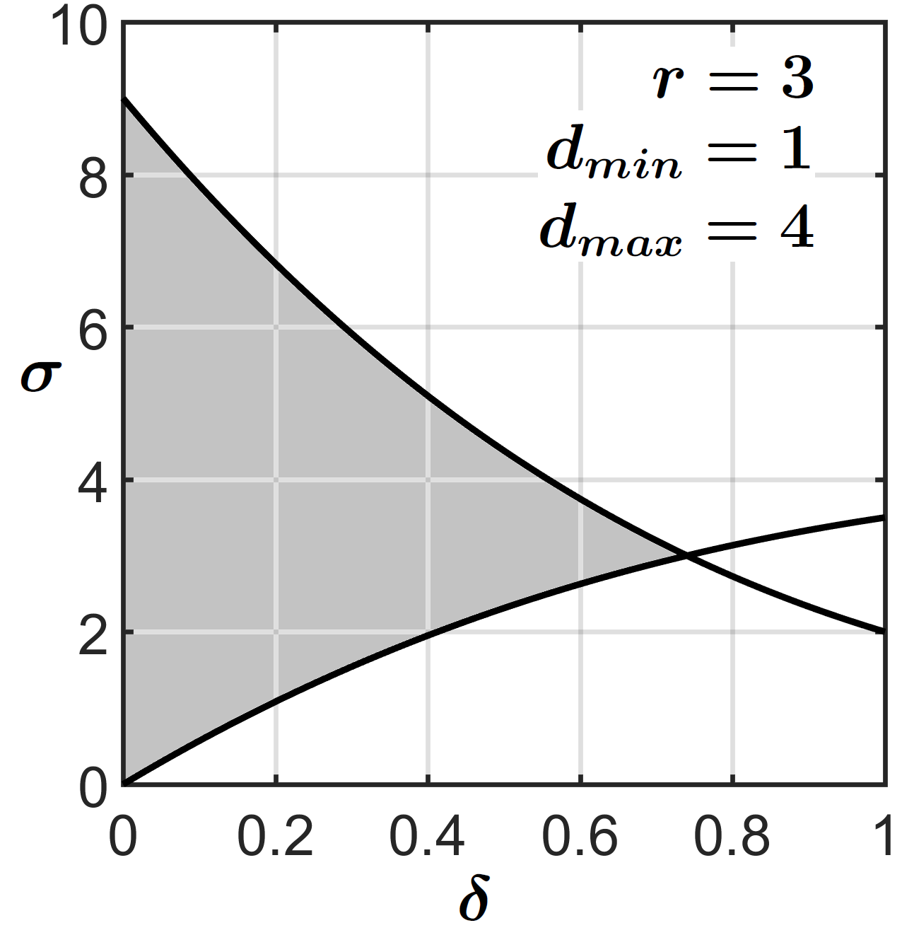

Remark 10.
(Failure of unconditional stability for SBDF and orders ) The necessary conditions for unconditional stability require that the generalized eigenvalues . The formulas from Proposition 6.1 lead to the requirement that:
These two inequalities cannot be simultaneously satisfied if , where is given by , , for orders , respectively. Note that is (up to ) a measure of the ratio . As a result, if the ratio between the maximum and minimum diffusion coefficient values exceed , then SBDF cannot provide unconditional stability for splittings of the form (6.5).
Remark 11.
(Overcoming limitations for SBDF and orders ) The formulas (6.14) provide a way to overcome the unconditional stability limitations encountered with SBDF methods for variable coefficient diffusion problems — regardless of the diffusion coefficient .
To demonstrate that the new approach works in practice, we conduct a convergence test of equation (6.4) with the variable diffusion coefficient
This ratio exceeds the value that can be stabilized by SBDF (see Remark 10). Using a value of in (6.14), and order yields the ImEx and splitting parameters . Since the unconditional stability region becomes smaller as the order increases, using automatically guarantees unconditional stability for all orders . We manufacture the forcing to generate an exact solution
| (6.15) |
run up to final time . The multistep scheme is initialized with the exact data: for . The spatial resolution is .
Table 1 shows the error , using the discrete maximum norm , capped at . Convergence rates for are reported. Note that with , the diffusive time step restriction is . Hence, time steps can be used that are orders of magnitude larger than those required by an explicit scheme. This highlights the benefits of unconditional stability when performing computations with progressively smaller grids.
| Num. | Error | Rate | Error | Rate | Error | Rate | Error | Rate | Error | Rate | |
|---|---|---|---|---|---|---|---|---|---|---|---|
| Steps | |||||||||||
| 5 | 7.9e+00 | - | 4.7e+01 | - | 3.4e+02 | - | 9.0e+02 | - | 8.8e+02 | - | |
| 10 | 3.4e+00 | 1.2 | 6.7e+01 | -0.5 | 4.9e+02 | -0.5 | 2.2e+03 | -1.3 | 4.3e+03 | -2.3 | |
| 20 | 4.3e+00 | -0.4 | 2.4e+01 | 1.5 | 5.6e+02 | -0.2 | 3.7e+03 | -0.7 | 6.3e+03 | -0.5 | |
| 40 | 1.3e+00 | 1.7 | 3.5e+01 | -0.5 | 5.4e+02 | 0.1 | 6.3e+03 | -0.8 | 5.8e+04 | -3.2 | |
| 80 | 6.9e-01 | 1.0 | 7.1e+00 | 2.3 | 1.3e+01 | 5.4 | 7.4e+02 | 3.1 | 6.0e+03 | 3.3 | |
| 160 | 2.7e-01 | 1.4 | 1.0e+00 | 2.8 | 1.1e+01 | 0.2 | 5.3e+01 | 3.8 | 5.7e+01 | 6.7 | |
| 320 | 2.2e-01 | 0.3 | 6.0e-01 | 0.8 | 2.5e+00 | 2.2 | 2.8e+00 | 4.2 | 7.1e+00 | 3.0 | |
| 640 | 2.9e-01 | -0.4 | 5.3e-01 | 0.2 | 6.3e-01 | 2.0 | 1.5e-01 | 4.3 | 4.0e-01 | 4.1 | |
| 1280 | 2.5e-01 | 0.2 | 2.2e-01 | 1.3 | 5.0e-02 | 3.7 | 3.6e-02 | 2.1 | 2.5e-02 | 4.0 | |
| 2560 | 1.6e-01 | 0.6 | 5.6e-02 | 2.0 | 4.9e-03 | 3.4 | 3.5e-03 | 3.4 | 2.8e-04 | 6.4 | |
| 5120 | 9.1e-02 | 0.8 | 1.2e-02 | 2.2 | 8.5e-04 | 2.5 | 2.0e-04 | 4.1 | 1.0e-05 | 4.8 | |
| 1.0e+04 | 4.8e-02 | 0.9 | 2.8e-03 | 2.1 | 1.3e-04 | 2.7 | 1.1e-05 | 4.2 | 3.8e-07 | 4.7 | |
| 2.0e+04 | 2.5e-02 | 1.0 | 6.7e-04 | 2.1 | 1.8e-05 | 2.9 | 6.1e-07 | 4.2 | 1.3e-08 | 4.9 | |
| 4.1e+04 | 1.2e-02 | 1.0 | 1.6e-04 | 2.0 | 2.4e-06 | 2.9 | 3.6e-08 | 4.1 | 1.1e-09 | 3.5 | |
| 8.2e+04 | 6.3e-03 | 1.0 | 4.0e-05 | 2.0 | 3.0e-07 | 3.0 | 2.2e-09 | 4.0 | 1.4e-09 | - | |
| 1.6e+05 | 3.1e-03 | 1.0 | 9.8e-06 | 2.0 | 3.8e-08 | 3.0 | 2.3e-10 | 3.3 | 2.8e-09 | - |
6.3 A nonlinear example: Diffusion in porous media and anomalous diffusion rates
Thus far, the unconditional stability theory has been applied exclusively to linear problems. Now we use the linear theory as a guide for choosing in nonlinear problems, and numerically demonstrate that the new concepts work. In spirit, the presented methodology shares some similarities with Rosenbrock methods (chapter VI.4, [29]) in that it also avoids nonlinear implicit terms by means of a properly chosen linear implicit term. A key difference — other than the fact that Rosenbrock methods are multistage schemes — is that we do not compute Jacobian matrices (which can be dense and time-dependent), but rather always invert a simple constant coefficient matrix determined from the theory. Hence, the new approach offers more flexibility for choosing efficiency-based implicit terms.
We consider a nonlinear model for a gas diffusing into a porous medium [46, 52]:
Here is the intrinsic permeability of the medium, and is the effective viscosity. Combined with the equation of state , where is the adiabatic constant ( for an ideal monatomic gas), the porous media equation takes the form:
| (6.16) |
The constant may, without loss of generality, be set to any positive value by re-scaling time.
We discretize (6.16) in three space dimensions using Fourier modes on the periodic domain . Our goal is to achieve unconditional stability by choosing the discrete matrix proportional to the constant coefficient Laplacian (which is easy to treat implicitly). This approach then avoids an implicit treatment of nonlinear terms, thereby bypassing the need for nonlinear solvers. Due to the nonlinearity in the diffusion coefficient, our choice of via the formulas (6.14) requires estimates for the maximum and minimum values of the solution over the simulation. At first glance, it may seem troubling to require time stepping parameters based on the solution; however this is not unusual — numerical simulations for nonlinear PDEs often require choosing a time step that may depend on the solution.
To test the approach for unconditional stability and accuracy, we perform convergence tests of (6.16) with and , using the manufactured solution
| (6.17) |
We initialize the ImEx scheme with the exact initial data for . We estimate the maximum and minimum value of the nonlinear diffusion coefficient:
Using formulas (6.14) with , , , and (so that the resulting scheme is stable for all orders through ), yields: .
Table 2 shows the numerical error , using the discrete norm evaluated at the final time , using grid points (). In addition to confirming the convergence orders, the table demonstrates that the scheme is stable for -values far larger than required by a fully explicit scheme. Moreover, we have confirmed the observations using other values and other manufactured solutions (not shown here).
| Num. | Error | Rate | Error | Rate | Error | Rate | Error | Rate | Error | Rate | |
|---|---|---|---|---|---|---|---|---|---|---|---|
| Steps | |||||||||||
| 8 | 1.0e+00 | - | 8.3e-01 | - | 6.4e-02 | - | 9.7e-02 | - | 3.4e-04 | - | |
| 16 | 7.7e-01 | 0.4 | 3.8e-01 | 1.1 | 3.4e-02 | 0.9 | 2.2e-02 | 2.1 | 8.1e-04 | -1.2 | |
| 32 | 5.0e-01 | 0.6 | 8.3e-02 | 2.2 | 8.6e-03 | 2.0 | 1.9e-03 | 3.6 | 1.2e-04 | 2.7 | |
| 64 | 2.6e-01 | 0.9 | 1.5e-02 | 2.4 | 1.4e-03 | 2.6 | 1.2e-04 | 4.0 | 7.6e-06 | 4.0 | |
| 128 | 1.3e-01 | 1.0 | 3.6e-03 | 2.1 | 1.9e-04 | 2.8 | 6.6e-06 | 4.2 | 3.0e-07 | 4.7 | |
| 256 | 6.4e-02 | 1.0 | 8.6e-04 | 2.1 | 2.5e-05 | 2.9 | 3.8e-07 | 4.1 | 1.3e-08 | 4.5 | |
| 512 | 3.2e-02 | 1.0 | 2.1e-04 | 2.0 | 3.2e-06 | 3.0 | 2.2e-08 | 4.1 | 6.2e-09 | - | |
| 1024 | 1.6e-02 | 1.0 | 5.2e-05 | 2.0 | 4.0e-07 | 3.0 | 9.8e-10 | 4.5 | 1.2e-08 | - | |
| 2048 | 7.8e-03 | 1.0 | 1.3e-05 | 2.0 | 5.0e-08 | 3.0 | 6.9e-10 | - | 2.4e-08 | - |
Now we conduct a test in which the nonlinear behavior is natural to equation (6.16): a decaying/spreading profile without forcing. We use a Gaussian as initial data, which is not exactly periodic, but is sufficiently resolved in space using Fourier modes () to carry out temporal convergence studies. We choose , and set , which for the given initial data will lead to dynamics that evolve on an time scale. Using (6.14) with , , , and , we obtain . To generate the initial data required to start the high-order multistep methods, we use the low order ( and ) unconditionally stable schemes with many subgrid time steps.
Table 3 provides a verification for the test, by computing the convergence rate estimate
| (6.18) |
where denotes the discrete solution at computed using time step . Table 3 confirms that at small values, converges to the order of the scheme.
| , | 1.22 | 1.58 | 1.52 | 1.28 | 1.14 | 1.07 | 1.03 | 1.02 | 1.01 |
|---|---|---|---|---|---|---|---|---|---|
| , | 0.39 | 5.12 | 2.06 | 2.02 | 1.96 | 1.95 | 1.96 | 1.97 | 1.98 |
| , | 1.38 | 3.54 | 1.63 | 8.52 | 2.83 | 2.74 | 2.81 | 2.88 | 2.93 |

Finally, guided by the data in Table 3, we choose a time step , and compute the solution towards (i.e. merely 32 time steps). Figure 8 visualizes level sets of the solution for different times and compares them to a reference solution (obtained using the fully explicit, second-order scheme with , i.e. Adams-Bashforth, with , i.e. 65536 time steps). The unconditionally stable method is successfully capturing the solution, albeit using very large time steps.
Meanwhile, Figure 9 highlights the nonlinear effect (anomalous diffusion) in the solution with plots of the decay rate of the peak relative to the mean value . For reference, the decay rate for a linear constant coefficient diffusion problem () is shown as well. The plot shows, against the reference solution, the ImEx schemes with (64 time steps, a small error) and (256 time steps, visually indistinguishable).

7 Incompressible channel flow
In this section we perform a study that zooms in on the question of unconditional stability for ImEx splittings that arise in fluid dynamics problems. Specifically, for the time-dependent Stokes equation in a channel geometry, we devise unconditionally stable ImEx schemes that treat the pressure explicitly and viscosity implicitly. High-order ImEx schemes that are provably unconditionally stable for the incompressible Navier-Stokes equations are notoriously difficult to attain (see for instance [27, 48, 49]). This study highlights some peculiar challenges that arise with ImEx schemes for incompressible flows, for instance that unconditional stability may depend on model parameters such as the shape and size of the domain. The new unconditional stability theory may provide new ways to stabilize operator splittings in fluid dynamics applications that might otherwise be unstable.
It is worth mentioning that in fluid flow, the alternative to unconditional stability may not necessarily be detrimental (in fact, the situation here is of that type). For instance, when unconditional stability is not attained, an ImEx approach may still provide competitive stability benefits, by incurring a time step restriction that is (i.e. independent on the spatial mesh), and thus not stiff. This type of stability restriction has been recently referred to as quasiunconditional stability [10, 11] (and has been applied to the compressible Navier-Stokes equations in an alternate direction implicit (ADI) setting). Nonetheless the question of whether unconditionally stable schemes can be devised is of interest, as in other situations the lack of unconditional stability may not be as forgiving as the quasiunconditional stability scenario.
We focus on reformulations of the incompressible Navier-Stokes equations [32, 38, 39, 49, 56], that take the form of a pressure Poisson equation (PPE) system (sometimes also referred to as an extended Navier-Stokes system). They replace the divergence-free constraint by a non-local pressure operator (defined via the solution of a Poisson equation), and thus allow for the application of time-stepping schemes without having to worry about constraints. In contrast to projection methods [39, 49, 32, 56], PPE systems are not based on fractional steps, and thus allow in principle for arbitrary order in time. In turn, the use of ImEx schemes allows for an explicit treatment of the pressure — which (in contrast to fully implicit time-stepping) avoids large saddle-point problems in which velocity and pressure are coupled together. The challenge is that the explicit pressure term may become stiff (because it can be recast as a function of the viscosity term [39, 56]).
For simplicity, we restrict this presentation to the linear Navier-Stokes equations (i.e. without the advection terms), because these equations already capture the key challenges arising from the interaction between viscosity and pressure. One could also investigate (unconditional) stability for incompressible flows with advection terms; however we do not pursue this here. For a two dimensional domain , we use the PPE reformulation by Johnston and Liu [39, 38] for problems with no-slip boundary conditions:
| (7.1) |
where is the solution of
| (7.2) |
Equation (7.1) is the standard momentum equation for the velocity field , while equation (7.2) is the PPE reformulation for the pressure, acting to keep the flow incompressible. Note that the last requirement in equation (7.2) is added to uniquely define the pressure. Here, is the outward facing normal on , and is the body force. The viscosity terms and are the stiff terms that are treated implicitly (matrix ), while the pressure terms are linear functions of the velocity that are treated explicitly (matrix ). We consider a channel geometry, , that is periodic in the -direction.
The simple geometry allows us to solve for the pressure analytically, and convert equations (7.1)–(7.2) into a non-local PDE for the velocity . This simplifies the computation of the set and provides fundamental insight into why existing ImEx splittings that treat the viscosity terms implicitly and pressure terms explicitly may become unstable. In more general problems, one would of course need to conduct a full spatial discretization of equations (7.1)–(7.2), and apply the recipes described in §4 to the resulting large ODE system. It is important to note that, while theoretical insights are less clear in that situation, there is no fundamental problem with applying the methodology.
To derive the non-local PDE for the velocity , we start off by setting (unconditional stability does not depend on the forcing). Because is periodic in the -direction, we conduct a Fourier expansion in the -direction and set and . The system (7.1)–(7.2) then becomes:
| (7.3) | ||||
| (7.4) |
The allowable wave numbers are given by and natural numbers . The pressure equation (7.4) is uniquely solvable for all ; while for , the integral constraint in (7.2), together with (7.4), fixes . For , equation (7.4) can be solved analytically to obtain:
| (7.5) |
The pressure can then be substituted back into equation (7.3) to yield a non-local PDE for the horizontal velocity (for ):
| (7.6) |
Solving equation (7.6) for at every wave number then allows one to reconstruct . In a similar fashion, one can use (7.5) to reconstruct . Once either or is known, the vertical velocity can then be obtained by solving either (i) the -component of equation (7.3) with the pressure as a prescribed forcing, or (ii) using the fact that the PPE reformulation automatically enforces the divergence constraint so that . Collectively, the solutions from (7.5)–(7.6) solve the original PDEs (7.1)–(7.2) with . Thus, devising unconditionally stable ImEx splittings for (7.6) can be used as a guide for stabilizing discretizations of the full equations (7.1)–(7.2).
7.1 Numerical discretization and ImEx splitting for equation (7.6)
In line with prior examples, we seek ImEx splittings of equation (7.6) in which the pressure terms are treated explicitly, while a portion of the viscosity is treated implicitly:
| (7.7) |
Although equation (7.6) is a non-local PDE, the highest derivative degree is so that the splitting (7.7) still adheres to the guidelines in Remark 6. As with prior discussions, the inclusion of the splitting parameter in (7.7) provides additional flexibility in devising stable schemes, compared to many existing splittings that effectively fix .
To obtain the matrices we discretize the -direction using equispaced grid points , and spacing , so that , for . A standard 3-point finite difference stencil for (with Dirichlet boundary conditions at ) leads to the following discretization: , where
| (7.8) |
In a similar fashion, we set where is a matrix that computes the pressure. The matrix is built using equation (7.5) as
| (7.9) |
Here the vectors and approximate the derivatives and , and thus encode the boundary conditions . The vectors are discretizations of the functions
Note that for each fixed value of , the matrix is the sum of two rank- matrices.
7.2 Applying the unconditional stability theory to determine
Now we follow the guidelines in Remark 6 to determine . We directly focus on computing an appropriate set to be used in the stability theory.
Unlike prior examples, for the channel flow application considered here, the choice is most useful for the analysis of the sets. This is because the maximum size and shape of the sets are effectively independent of . In contrast, numerical experiments show that the sets arising from (7.7) tend to grow as . It is worth noting that is also motivated by [39], in which a version of the set was studied to prove that SBDF1 is unconditionally stable when applied to the channel flow PDEs (7.1)–(7.2). Here, we apply the full new unconditional stability theory to systematically investigate stability for high order schemes.
To compute , we use the scaling property from Remark 5 to write
| (7.10) |
and use Chebfun’s numerical range (field of values) routine [20] to compute ; from which is obtained via a shift and re-scaling. Note that Chebfun employs an algorithm due to Johnson [37] that reduces the computation of to a collection of eigenvalue computations.
A theoretical study of the set where continuum operators and were used instead of discrete matrices (note that the set is still defined using operators), was carried out in part of the work [39]. They showed that the set , using continuum operators, was real and contained in the interval . Our numerical computations of also show that for each fixed value of , the sets are within a discretization error (at most ) of the interval .
To quantify the region that occupies along the real axis, let
Figure 10 plots the sets for and grid spacing . Figure 11 plots for different wave numbers (where is a special case and excluded from the plot) and grids . The plot shows that decreases (monotonically) with increasing — which is important for the simultaneous stabilization of all wave numbers that arise in a channel geometry. The minimum value is always zero, i.e. .


Since the sets lie along the real axis, the procedure for choosing parallels that of the diffusion example in §6.2. For instance, we can use equations (6.12) (for ) and (6.14) (for ) via the substitutions and to ensure that . This approach determines the parameters that ensure unconditional stability for the PDE (7.9) for one fixed wave number . In practice, however, stabilizing equation (7.6) for a channel geometry requires that it be unconditionally stable for all allowable wave numbers . The following remark shows that it suffices to ensure unconditional stability for the smallest non-zero wave number (which then stabilizes all others).
Remark 12.
(Choosing one that works for all wave numbers ) Unconditional stability for equations (7.1)–(7.2) corresponds to ensuring that (7.6) is stable for all modes . Here we argue why it suffices to ensure that only the smallest mode is stable, i.e., to require that , where is the smallest positive wave number.
To show this, we use the simple property that the sets may be written as a numerical range. First, one can view the simultaneous solution of equation (7.6) over all allowable , as solving one very large system of equations with matrices and that are written as direct sums. Specifically, write and , where the direct sum is over the wave numbers and natural numbers (i.e. are infinite block diagonal matrices with each block being or ). Now use the fact that the set may be written as a numerical range (see Remark 2) — and that the numerical range of the direct sum of two matrices is the convex hull of their two numerical ranges, i.e. . As a result, the set is the convex hull of the sets over all allowable wave numbers. Lastly, we observe that the set contains (up to at most an error ) each of the sets for all and . This shows that the convex hull of the sets over all is approximately equal to the set . Specifically:
- •
For the mode , we have . Hence is a single point contained in the set .
- •
The matrices and are even functions of . Hence the sets are the same for both values.
- •
Hence we have that , where the sign (as opposed to an sign) denotes the fact that there may be an error.
Based on this important insight, we now choose for a channel geometry of length and smallest positive wave number . For grid size , the set is obtained by inserting the values and (see Figure 11) into equation (7.10). A crucial observation is that the largest and smallest generalized eigenvalues equal the maximum and minimum values of , see Figure 11 — and the gap between these generalized eigenvalues exceeds the unconditional stability capabilities of SBDF3 (see Remark 10). Hence, the new coefficients (i.e. ) must be used to achieve unconditional stability. Using a gap parameter of , order , and values , in equation (6.14), leads to . Figure 12 verifies that this choice in fact satisfies the sufficient conditions for unconditional stability.

We conclude this section with a few important observations. For a fixed value of , the maximum value remains bounded below as . This implies that one value of may be used to stabilize an entire family of splittings. On the other hand, the sets do depend on — and Figure 11 implies that the sets (and also the generalized eigenvalues ) become large when . This observation is important because it implies that designing unconditionally stable schemes requires a choice of that depends on the domain size , and also on the fact that the domain is a channel geometry.
A natural question then arises: what values can take for a general fluid dynamics problem? Because the set may depend on the geometry shape (for instance whether has corners, see [17]) and size of the computational domain, one would expect that numerical computations may be required to determine or estimate . For instance, one may perform a few rapid computations of using a coarse mesh (i.e. large ) and thus small matrices and , to obtain a guide for determining the parameters for the fully resolved problem.
8 Conclusions and outlook
With this work on unconditionally stable ImEx multistep methods we wish to stress two key messages: first, we advocate to conduct the selection of the ImEx splitting and selection of the time-stepping scheme in a simultaneous fashion; and second, it is often possible to achieve unconditional stability in significantly more general settings than one might think at first glance.
The examples and applications discussed herein may serve as a blueprint for how to approach many other types of problems, by using the new stability theory and new ImEx schemes to determine feasible and optimal parameters that characterize the scheme and splitting, respectively.
The theoretical foundations of this work establish necessary and sufficient conditions for unconditional stability, resulting from unconditional stability diagrams (that depend only on the scheme) and computable matrix quantities (that depend only on the ImEx splitting). This analysis is then used to explain fundamental limitations of the popular SBDF schemes. In particular, it is shown why SBDF can frequently not be extended beyond first or second order — and how the new schemes can overcome this barrier.
The variable coefficient and nonlinear diffusion examples highlight the practical impact that the new methodology can bring: being able to treat problems whose stiff terms are challenging to invert, without stiff time step restrictions and without having to conduct challenging solves. In addition, the theory serves to provide some fundamental insight into unconditional stability (or breakdown thereof) in incompressible fluid flow simulations.
A key limitation of this work is the formal restriction to positive definite matrices . This excludes many splittings that would be warranted for intrinsically non-symmetric problems, such as advection or dispersion. Regarding this limitation, it should first be noted that much of the theory persists when the assumptions on are relaxed (for instance, may be a normal matrix with eigenvalues having complex arguments that are not too large). Second, the extension of the theory to truly non-symmetric is an important subject of future work.
Acknowledgments
The authors wish to acknowledge support by the National Science Foundation through grants DMS–1719640 (B. Seibold and D. Zhou) and DMS–1719693 (D. Shirokoff). D. Shirokoff was supported by a grant from the Simons Foundation ().
Appendix A Proof of Proposition 6.1
Throughout this section we suppress the subscript on the matrices , and simply write . We start with computing the set
| (A.1) | ||||
| (A.2) |
In the expression in (A.2), we have used the fact that the derivative matrix is skew-symmetric . Note that is invertible on the space (i.e. is orthogonal to — which is the nullspace of ). Making the change of variables in (A.2), we observe that as varies over , varies over . This yields:
where . Since , each value is real and confined to the region (note that because , not all vectors are allowed — only those having zero mean). Combining the results leads to the following inequality:
Hence, the set is real and bounded by:
This concludes the first part of the proof. To prove the eigenvalue bounds on , the upper bound estimates (i.e. the bounds overestimating the largest and underestimating the smallest ) follow directly from using the established bounds on with the fact that . Thus, it suffices to prove only the lower bounds. We are interested in bounding the eigenvalues of with eigenvectors restricted to . Substituting and into the eigenvalue equation yields:
As before, let , which is an invertible transformation on . Then
or alternatively
| (A.3) |
for some . We now solve equation (A.3) for two separate cases:
Case 1: . Here for all . This is only possible if for all , i.e. one has a constant coefficient diffusion, and thus identically. Dotting (A.3) through by further shows that , thereby forcing all . Hence, Proposition 6.1 is satisfied (trivially) because and .
Case 2: . In this case, we solve equations (A.3) by first writing the components of in terms of the unknown eigenvalue :
Applying the constraint to the vector , shows that the eigenvalues are roots to the following equation:
Ordering the poles of along the real axis from smallest to largest shows that there is at least one root of between the smallest two values (or largest two values) of . Hence, Proposition 6.1 follows.
Appendix B Formulas for the ImEx coefficients
| Order | |||||
|---|---|---|---|---|---|
| 1 | . | . | |||
| . | . | 1 | (-1) | ||
| . | . | 0 |
| Order | |||||
|---|---|---|---|---|---|
| 2 | . | ||||
| . | 1 | ||||
| . | 0 |
| Order | |||||
|---|---|---|---|---|---|
| 3 | |||||
| 1 | |||||
| 0 |
| Order | ||||
|---|---|---|---|---|
| 4 | . | |||
| . | 1 | |||
| . | 0 | |||
| Order | |||
|---|---|---|---|
| 5 | |||
| 1 | |||
| 0 | |||
References
- [1] A. Abdulle and A. A. Medovikov, Second order Chebyshev methods based on orthogonal polynomials, Numer. Math., 90 (2001), pp. 1–18.
- [2] G. Akrivis, Implicit-explicit multistep methods for nonlinear parabolic equations, Math. Comput., 82 (2012), pp. 45–68.
- [3] G. Akrivis, M. Crouzeix, and C. Makridakis, Implicit-explicit multistep finite element methods for nonlinear parabolic problems, Math. Comput., 67 (1998), pp. 457–477.
- [4] , Implicit-explicit multistep methods for quasilinear parabolic equations, Numer. Math, 82 (1999), pp. 521–541.
- [5] G. Akrivis and F. Karakatsani, Modified implicit-explicit BDF methods for nonlinear parabolic equations, BIT Numer. Math., 43 (2003), pp. 467–483.
- [6] M. Anitescu, W. Layton, and F. Pahlevani, Implicit for local effects, explicit for nonlocal is unconditionally stable, ETNA, 18 (2004), pp. 174–187.
- [7] U. Ascher, S. J. Ruuth, and B. Wetton, Implicit-explicit methods for time dependent partial differential equations, SIAM J. Numer. Anal., 32 (1995), pp. 797–823.
- [8] V. Badalassi, H. Ceniceros, and S. Banerjee, Computation of multiphase systems with phase field models, J. Comput. Phys., 190 (2003), pp. 371–397.
- [9] A. Bertozzi, N. Ju, and J.-W. Lu, A biharmonic-modified forward time stepping method for fourth order nonlinear diffusion equations, Discrete and Continuous Dynamical Systems, 29 (2011), pp. 1367–1391.
- [10] O. P. Bruno and M. Cubillos, Higher-order in time quasi-unconditionally stable ADI solvers for the compressible Navier-Stokes equations in 2D and 3D curvilinear domains, J. Comput. Phys., 307 (2016), pp. 476–495.
- [11] , On the quasi-unconditional stability of BDF-ADI solvers for the compressible Navier-Stokes equations, SIAM J. Numer. Anal., 55 (2017), pp. 892–922.
- [12] O. P. Bruno and E. Jimenez, Higher-order linear-time unconditionally stable ADI methods for nonlinear convection-diffusion PDE systems, J. Fluids Eng., 136 (2014), pp. 060904–060904–7.
- [13] O. P. Bruno and M. Lyon, High-order unconditionally stable FC-AD solvers for general smooth domains I. basic elements, J. Comput. Phys., 229 (2010), pp. 2009–2033.
- [14] , High-order unconditionally stable FC-AD solvers for general smooth domains II. Elliptic, parabolic and hyperbolic PDEs; theoretical considerations, J. Comput. Phys., 229 (2010), pp. 3358–3381.
- [15] H. Ceniceros, A semi-implicit moving mesh method for the focusing nonlinear Schroedinger equation, Comm. on Pure and Appl. Anal., 1 (2002), pp. 1–14.
- [16] A. Christlieb, J. Jones, K. Promislow, B. Wetton, and M. Willoughby, High accuracy solutions to energy gradient flows from material science models, J. Comput. Phys., 257 (2014), pp. 193–215.
- [17] E. Cozzi and R. L. Pego, On optimal estimates for the Laplace-Leray commutator in planar domains with corners, Proc. Amer. Math. Soc., 139 (2011), pp. 1691–1706.
- [18] M. Crouzeix, Une méthode multipas implicite-explicite pour l’approximation des équations d’évolution paraboliques, Numer. Math, 35 (1980), pp. 257–276.
- [19] J. Douglas and T. Dupont, Alternating-direction Galerkin methods on rectangles, in Numerical Solution of Partial Differential Equations, B. Hubbard, ed., vol. II, College Park, Md., 1971, SYNSPADE-1970, Univ. of Maryland, Academic Press, New York, pp. 133–213.
- [20] T. A. Driscoll, N. Hale, and L. N. Trefethen, eds., Chebfun Guide, Pafnuty Publications, Oxford, 2014.
- [21] L. Duchemin and J. Eggers, The explicit-implicit-null method: removing the numerical instability of PDEs, J. Comput. Phys., 263 (2014), pp. 37–52.
- [22] M. Elsey and B. Wirth, A simple and efficient scheme for phase field crystal simulation, M2AN, 47 (2013), pp. 1413–1432.
- [23] D. Eyre, Unconditionally gradient stable time marching the Cahn-Hilliard equation, in Computational and Mathematical Models of Microstructural Evolution, J. W. Bullard, R. Kalia, M. Stoneham, and L. Chen, eds., vol. 53, Warrendale, PA, USA, 1998, Materials Research Society, pp. 1686–1712.
- [24] J. Frank, W. Hundsdorfer, and J. Verwer, On the stability of IMEX LM methods, Appl. Numer. Math., 25 (1997), pp. 193––205.
- [25] K. Glasner and S. Orizaga, Improving the accuracy of convexity splitting methods for gradient flow equations, J. Comput. Phys., 315 (2016), pp. 52–64.
- [26] Z. Guan, J. Lowengrub, C. Wang, and S. Wise, Second-order convex splitting schemes for periodic nonlocal Cahn-Hilliard and Allen-Cahn equations, J. Comput. Phys., 277 (2014), pp. 48–71.
- [27] J.-L. Guermond and P. Minev, High-order time stepping for the incompressible Navier-Stokes equations, SIAM J. Sci. Comput., 36 (2015), pp. A2656–A2681.
- [28] E. Hairer, S. P. Nørsett, and G. Wanner, Solving ordinary differential equations I: Nonstiff problems, Springer-Verlag, Berlin, second ed., 1987.
- [29] E. Hairer and G. Wanner, Solving ordinary differential equations II: Stiff and differential-algebraic problems, Springer-Verlag, Berlin, second ed., 1991.
- [30] T. Heister, M. A. Olshanskii, and L. G. Rebholz, Decoupled, unconditionally stable, higher order discretizations for MHD flow simulation, J. Sci. Comput., 71 (2017), pp. 21–43.
- [31] , Unconditional long-time stability method for the 2D Navier-Stokes equations, Numer. Math., 135 (2017), pp. 143–167.
- [32] W. D. Henshaw, A fourth-order accurate method for the incompressible Navier-Stokes equations on overlapping grids, J. Comput. Phys., 113 (1994), pp. 13–25.
- [33] A. Horn and C. Johnson, Topics in matrix analysis, Cambridge University Press, 1991.
- [34] W. Hundsdorfer and J. Verwer, Numerical solution of time-dependent advection-diffusion-feaction equations, Springer Series in Comput. Math. 33, Springer, 2003.
- [35] R. Jeltsch and O. Nevanlinna, Stability of explicit time discretizations for solving initial value problems, Numer. Math., 37 (1981), pp. 61–91.
- [36] , Stability and accuracy of time discretizations for initial value problems, Numer. Math., 40 (1982), pp. 245–296.
- [37] C. R. Johnson, Numerical determination of the field of values of a general complex matrix, SIAM J. Numer. Anal., 15 (1978), pp. 595–602.
- [38] H. Johnston and J.-G. Liu, A finite difference method for incompressible flow based on local pressure boundary conditions, J. Comput. Phys., 180 (2002), pp. 120–154.
- [39] , Accurate, stable and efficient Navier-Stokes solvers based on explicit treatment of the pressure term, J. Comput. Phys., 199 (2004), pp. 221–259.
- [40] L. Ju, J. Zhang, L. Zhu, and Q. Du, Fast explicit integration factor methods for semilinear parabolic equations, J. Sci. Comput., 62 (2015), pp. 431–455.
- [41] G. Karniadakis, M. Israeli, and S. A. Orszag, High-order splitting methods for the incompressible Navier-Stokes equations, J. Comput. Phys., 97 (1991), pp. 414–443.
- [42] A.-K. Kassam and L. N. Trefethen, Fourth-order time-stepping for stiff PDEs, SIAM J. Sci. Comput., 26 (2005), pp. 1214–1233.
- [43] J. Kim and P. Moin, Application of a fractional step method to incompressible Navier-Stokes equations, J. Comput. Phys., 59 (1985), pp. 308–323.
- [44] T. Koto, Stability of implicit-explicit linear multistep methods for ordinary and delay differential equations, Front. Math. China, 4 (2009), pp. 113–129.
- [45] W. Layton and C. Trenchea, Stability of two IMEX methods, CNLF and BDF2-AB2, for uncoupling systems of evolution equations, Appl. Numer. Math., 62 (2012), pp. 112––120.
- [46] L. S. Leibenzon, General problem of the movement of a compressible fluid in a porous media, Izv. Akad. Nauk SSSR, Geography and Geophysics, 9 (1945), pp. 7–10. (Russian).
- [47] R. J. LeVeque, Finite difference methods for ordinary and partial differential equations: Steady-state and time-dependent problems, SIAM, Philadelphia, first ed., 2007.
- [48] J.-G. Liu, J. Liu, and R. L. Pego, Stability and convergence of efficient Navier-Stokes solvers via a commutator estimate, Comm. Pure Appl. Math., 60 (2007), pp. 1443–1487.
- [49] , Stable and accurate pressure approximation for unsteady incompressible viscous flow, J. Comput. Phys., 229 (2010), pp. 3428–3453.
- [50] P. A. Milewski and E. G. Tabak, A pseudo-spectral algorithm for the solution of nonlinear wave equations, SIAM J. Sci. Comput., 21 (1999), pp. 1102–1114.
- [51] M. L. Minion, Semi-implicit spectral deferred correction methods for ordinary differential equations, Commun. Math Sci., 1 (2003), pp. 471–500.
- [52] M. Muskat, The flow of homogeneous fluids through porous media, McGrawHill, New York, 1937.
- [53] R. Rosales, B. Seibold, D. Shirokoff, and D. Zhou, Unconditional stability for multistep ImEx schemes – Theory, SIAM J. Numer. Anal., 55 (2017), pp. 2336–2360.
- [54] G. Sheng, T. Wang, Q. Du, K. Wang, Z. Liu, and L. Q. Chen, Coarsening kinetics of a two phase mixture with highly disparate diffusion mobility, Commun. Comput. Phys., 8 (2010), pp. 249–264.
- [55] J. Shin, H. Lee, and J.-Y. Lee, Unconditionally stable methods for gradient flow using convex splitting Runge-Kutta scheme, J. Comput. Phys., 347 (2017), pp. 367–381.
- [56] D. Shirokoff and R. R. Rosales, An efficient method for the incompressible Navier-Stokes equations on irregular domains with no-slip boundary conditions, high order up to the boundary, J. Comput. Phys., 230 (2011), pp. 8619–8646.
- [57] P. Smereka, Semi-implicit level set methods for curvature and surface diffusion motion, J. Sci. Comput., 19 (2003), pp. 439–456.
- [58] L. N. Trefethen and D. Bau, Numerical Linear Algebra, SIAM, Philadelphia, 2000.
- [59] C. Trenchea, Second order implicit for local effects and explicit for nonlocal effects is unconditionally stable, Romai J., 12 (2016), pp. 163–178.
- [60] J. M. Varah, Stability restrictions on second order, three level finite difference schemes for parabolic equations, SIAM J. Numer. Anal., 17 (1980), pp. 300–309.
- [61] Y. Yan, W. Chen, C. Wang, and S. Wise, A second-order energy stable BDF numerical scheme for the Cahn-Hilliard equation, Commun. Comput. Phys., 23 (2018), pp. 572–602.