One-dependent colorings of the star graph

Finitely dependent processes have received considerable interest in probability theory and dynamical systems. They have a variety of applications including economic theory [17, 18], statistics [2, 6], queueing systems [9, 25], stochastic geometry [8], and biology [4, 21]. Early work of Ibragimov and Linnik [16] explored a representation of finitely dependent processes via block-factors. A block-factor can be expressed as a finite-range function of a family of independent and identically distributed random variables. It is straightforward that a block-factor is stationary finitely dependent, and they showed that the converse is true for Gaussian processes. This left the question of whether any stationary finitely dependent process is a block-factor for decades. It was not until the late 1980s that Aaronson, Gilat, Keane and de Valk [1] discovered stationary $1$-dependent processes which are not $2$-block-factors. There have now been a rich body of literature on finitely (and especially one-) dependent processes, with topics such as classical limit theory, examples in connection with integrable probability and combinatorial interpretations; see [3, 14] for an overview.

The constructions in [1] and many subsequent works are purely technical and counter-intuitive. An important question is whether ‘natural’ examples of finitely dependent processes are all block-factors. In fact, several works [7, 19, 20] assumed a block-factor assumption in the study of finitely dependent processes: if natural finitely dependent processes are block-factors, then there is little to be lost by making this assumption. In their groundbreaking work [14], Holroyd and Liggett considered stationary finitely dependent proper colorings, providing the first natural finitely dependent processes that are not any block-factors. Proper coloring has applications in computer science. Colors may represent time schedules for job tasks in a network, where any adjacent pair of job tasks are not permitted to conflict with each other. Finite dependence introduces a security benefit – an adversary can get access to information of some job tasks only within a fixed finite range. To proceed further, we need a few vocabularies.

In the last five years, there has been much effort in understanding stationary finitely dependent colorings of the integers, i.e. $V=\mathbb{Z}$ and $G$ is the infinite $2$-regular tree. It is obvious that stationary finitely dependent $2$-coloring of $\mathbb{Z}$ fails to exist. Holroyd, Schramm and Wilson [15] showed that there is no stationary $1$-dependent $3$-coloring of $\mathbb{Z}$. Holroyd and Liggett [14] found a stationary $1$-dependent $4$-coloring and a stationary $2$-dependent $3$-coloring of $\mathbb{Z}$, which imply the existence of stationary $k$-dependent $q$-colorings for all $k\geq 1$ and $q\geq 3$ except $(k,q)=(1,3)$ by splitting a color into further colors using external randomness. However, such constructed colorings are not symmetric under permutations of the colors for a general $q$. Further in [13], they constructed for each $q\geq 4$ a stationary $1$-dependent $q$-coloring which is invariant in law under permutations of the colors and under reflection. Precisely, they provided the following remarkable deletion-concatenation recursion for the cylinder probability $P^{*}$ of the $q$-coloring ${\bf x}\in[q]^{n}$ (which represents a sequence of consecutive colors along a path):

where $\widehat{\bf x}_{j}$ is obtained by deleting the $j^{th}$ entry of ${\bf x}$, and $C(n):=T_{n}(\sqrt{q}/2)$ for $n\geq 0$ and $D(n):=\sqrt{q}U_{n-1}(\sqrt{q}/2)$ for $n\geq 1$, with $T_{n}$ and $U_{n}$ the Chebyshev polynomials of the first and second kind respectively. More explicitly,

Later Holroyd, Hutchcroft and Levy [12] gave a probabilistic construction of the $1$-dependent $q$-coloring defined by (1) along with other stationary finitely dependent colorings of $\mathbb{Z}$ using the Mallows permutations. They also considered the problem of expressing a stationary finitely dependent coloring as a finitary factor of an independent and identically distributed sequence. See [5, 11] for other finitely dependent coloring models, and [10, 27] for recent progress on finitary factors.

As the readers may notice, recent works of finitely dependent colorings focused mostly on the integer case and its obvious extensions. For instance, it is easy to use the construction (1) to build a $1$-dependent $4^{d}$-coloring of $\mathbb{Z}^{d}$, which is stationary but is not invariant under all isometries of $\mathbb{Z}^{d}$. In fact, very little is known about ‘fully’ symmetric (or automorphism invariant) finitely dependent colorings of graphs such as $\mathbb{Z}^{d}$ for $d\geq 2$ and homogeneous trees. One main open problem is to find an automorphism invariant $1$-dependent coloring of $\mathbb{Z}^{d}$ for each $d\geq 2$, or more generally, of the $d$-regular tree for each $d\geq 3$. Note that any automorphism invariant coloring of $\mathbb{Z}^{d}$ or the $d$-regular tree (if it exists), when restricted to a copy of $\mathbb{Z}$, is a coloring of $\mathbb{Z}$ that is invariant under permutations of the colors. Moreover, it was conjectured in [12, 14] that the distribution (1) defines the unique $1$-dependent coloring which is invariant in law under permutations of the colors, under translation and reflection. So it is natural to look for a $1$-dependent coloring of an infinite graph such that

1. $(i)$

   the coloring is invariant in law under permutations of the colors;

2. $(ii)$

   the restriction to any path is distributed as (1).

As pointed out in [14], there is a close connection between proper colorings and hard-core processes. A hard-core process on $G$ is a process $(J_{v})_{v\in V}\in\{0,1\}^{V}$ such that almost surely we do not have $J_{u}=J_{v}=1$ whenever $u$ and $v$ are neighbors. So if $X$ is a $q$-coloring of $G$, then $J_{v}:=1_{\{X_{v}=x\}}$ defines a hard-core process for any given color $x\in[q]$; if $X$ is $1$-dependent, then so is $J$. As an immediate consequence, the number of colors needed for a $1$-dependent coloring of $G$ is bounded from below by $1/p_{h}(G)$, where

is referred to as the critical point. Motivated by the study of the repulsive lattice gas, Scott and Sokal [22, 23] showed that for any infinite connected graph $G$ of maximum degree $d$,

The lower bound in (4) is known to be achieved by the $d$-regular tree [24], which is a version of the Lovász local lemma. So any (symmetric) $1$-dependent coloring of the $d$-regular tree requires at least $d^{d}/(d-1)^{d-1}$ colors, e.g. $7$ colors for the $3$-regular tree, and $10$ colors for the $4$-regular tree or $\mathbb{Z}^{2}$. For $d=2$, the lower bound for the number of colors needed for a symmetric $1$-dependent coloring of $\mathbb{Z}$ is achieved by the construction (1). But it remains unknown whether one can find an automorphism invariant $1$-dependent $q$-coloring for any $q$ of the $d$-regular tree with $d>2$.

The purpose of this paper is to provide further study of symmetric $1$-dependent colorings of general graphs. As we will see later, this does not seem to be a simple task even going slightly beyond the integer case. Defining cylinder probabilities via recursion similar to (1) is arguably the most direct and promising way to construct any $1$-dependent coloring of a graph. However, the idea of deletion-concatenation is not easily replicated if some vertices have degree greater than $2$, and the question is how to genuinely concatenate its neighbors once a vertex is deleted. In view of this, we consider for any $d\geq 3$ the $d$-ray star graph and its subgraphs, which are building blocks for general graphs. Particular focus will be placed on the $3$-ray star graph.

The $d$-ray graph $\mathscr{S}^{d}$ has a distinguished vertex of degree $d$ and all the others of degree $2$, and it consists of $d$ rays ${\bf v}^{1}=(v_{11},v_{12},\ldots)$, ${\bf v}^{2}=(v_{21},v_{22},\ldots),\ldots$, and ${\bf v}^{d}=(v_{d1},v_{d2},\ldots)$, emanating from the distinguished vertex $v_{0}$. We also identify the $2$-ray star graph $\mathscr{S}^{2}$ with the integers. See Figure 1 below for a $3$-ray star graph.

Let $\mathbb{N}:=\{1,2,\ldots\}$ be the set of positive integers. For ${\bf n}:=(n_{1},\ldots,n_{d})\in\mathbb{N}^{d}$, let $\mathscr{S}^{d}_{\bf n}$ be the finite subgraph of the $d$-ray star graph, with $d$ rays of lengths $n_{1},\ldots,n_{d}$ respectively. Our first result gives an explicit formula for the critical point of $\mathscr{S}^{d}_{\bf n}$ for each $d\geq 2$ and ${\bf n}\in\mathbb{N}^{d}$, thus providing a lower bound for the number of colors needed for a symmetric $1$-dependent coloring of the $d$-ray star graph.

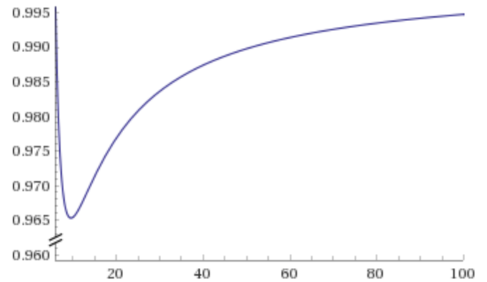
It is easy to derive from (7) that $p_{h}(\mathscr{S}^{2})=1/4$, $p_{h}(\mathscr{S}^{3})=\sqrt{5}-2$, $p_{h}(\mathscr{S}^{4})=\frac{1}{3}\bigg(2-11$ $\left(\frac{2}{9\sqrt{93}-47}\right)^{\frac{1}{3}}+\left(\frac{9\sqrt{93}-47}{2}\right)^{\frac{1}{3}}\bigg)$, and $p_{h}(\mathscr{S}^{d})\sim\ln d/d$ as $d\rightarrow\infty$. Table $1$ below displays the numerical values of $p_{h}(\mathscr{S}^{d})$ as $d$ ranges from $2$ to $11$.

TABLE 1. Numerical values of $p_{h}(\mathscr{S}^{d})$, $2\leq d\leq 11$.

Theorem 1.2 is essentially a consequence of [14, Lemma 24], which is related to the smallest real zero of the partition function or the independence polynomial of the hard-core model. The explicit formula (7) for the critical point of $\mathscr{S}^{d}$ is new. For ease of reference, we prove Theorem 1.2 in Section 3.

Recall that the lower bound in (4) is achieved by the $d$-regular tree, and an interesting question is whether the upper bound in (4) for $d\geq 3$ can also be achieved by some subgraph of the $d$-regular tree with at least one vertex of degree $d$. Since any infinite connected graph of maximum degree $d$ contains a copy of $\mathscr{S}^{d}_{(1,\ldots,1,n)}$ for each $n$, we get the following corollary.

Note that the bounds in (9) are tight, and the upper bound is improved for all $d\geq 4$. The formula (10) for $\lim_{n\to\infty}p_{h}(\mathscr{S}^{d}_{(1,\ldots,1,n)})$ is derived similarly as (7) for $p_{h}(\mathscr{S}^{d})$ (see Section 3.1). It is also easy to see that $(d-1)^{d-1}/d^{d}\sim 1/(ed)$ and $p_{\star}(d)\sim\ln d/d$ as $d\rightarrow\infty$. Table $2$ below displays the numerical values of $p_{\star}(d)$ as $d$ ranges from $2$ to $11$.

TABLE 2. Numerical values of $p_{\star}(d)$, $2\leq d\leq 11$.

Now we focus our attention on the $3$-ray star graph and its subgraphs. Recall that our goal is to find a $1$-dependent coloring of the graph which satisfies the conditions $(i)$-$(ii)$. According to Theorem 1.2, such a coloring requires at least $5$ colors. But constructing such a $q$-coloring for any $q\geq 5$ still seems to be far-fetched. A potentially less challenging task is to find a symmetric $1$-dependent coloring of the subgraph $\mathscr{S}^{3}_{(m,n,\infty)}$ for some finite $m,n$. Again by Theorem 1.2, it is easy to get a lower bound for the number of colors required for the coloring, e.g.

• •

  for $(m,n)=(1,1)$ or $(1,2)$, the number of colors needed is at least $4$;

• •

  for $m,n\geq 2$, the number of colors needed is bounded from below by $5$.

The next result shows that it is impossible to construct a $1$-dependent $4$-coloring of $\mathscr{S}^{3}_{(1,1,\infty)}$ and $\mathscr{S}^{3}_{(1,2,\infty)}$ which satisfies $(i)$-$(ii)$ above.

The proof of Proposition 1.4 is deferred to Section 4. Note that Proposition 1.4 does not exclude the possibility of finding a $1$-dependent $4$ coloring of $\mathscr{S}^{3}_{(1,1,\infty)}$ or $\mathscr{S}^{3}_{(1,2,\infty)}$ with restriction to any copy of $\mathbb{Z}$ a symmetric $1$-dependent $4$-coloring of $\mathbb{Z}$. Proving or disproving this fact are both of interest. If one proves such a coloring is impossible, it gives the first example where the lower bound for the number of colors specified by the inverse critical point is not attained. Otherwise, one can construct a $1$-dependent $4$-coloring whose restriction to ${\bf v}^{1}v_{0}{\bf v}^{2}$, ${\bf v}^{1}v_{0}{\bf v}^{3}$, ${\bf v}^{2}v_{0}{\bf v}^{3}$ is a symmetric coloring but different from that given by (1).

So far we have not seen any example of $1$-dependent coloring of an infinite graph other than $\mathbb{Z}$, which satisfies $(i)$-$(ii)$. Here we aim to construct the first such coloring of $\mathscr{S}^{3}_{(1,1,\infty)}$. Write $\begin{array}[]{c}\bf x\\[-3.0pt] x_{L}\,x_{0}\,x_{R}\end{array}$ for a generic $q$-coloring of $\mathscr{S}^{3}_{(1,1,n)}$, with ${\bf x}:=(x_{1},\ldots,x_{n})\in[q]^{n}$ and $x_{L},x_{0},x_{R}\in[q]$. Based on small cases computation, we arrive at the following construction which is in a similar flavor to (1) but in a more intricate way.

The proof of Theorem 1.5 is given in Section 5. Here are a few examples of cylinder probabilities: $P(121)=\frac{1}{q^{2}(q-1)}$, $P(123)=\frac{1}{q^{2}(q-2)}$,

Note that the construction (11) distinguishes whether $x_{L}=x_{R}$ or not. The case $x_{L}\neq x_{R}$ is specified by a deletion-concatenation recursion (11) which is similar to (1). Additional difficulties come from the subtraction recursion (11), where the nonnegativity is also not obvious. Theorem 1.5, together with Proposition 1.4 give a whole picture of symmetric $1$-dependent colorings of $\mathscr{S}^{3}_{(1,1,\infty)}$ which satisfy the additional condition (ii). However, we do not know any symmetric coloring of $\mathscr{S}^{3}_{(1,1,\infty)}$ which does not satisfy (ii). The situation is even more complicated for $1$-dependent colorings of $\mathscr{S}^{3}_{(m,n,\infty)}$ where at least one of $m,n$ is greater than $1$. It remains unknown whether one can find a $1$-dependent $q$-coloring for any $q\geq 5$ of $\mathscr{S}^{3}_{(1,2,\infty)}$ which satisfies the conditions $(i)$-$(ii)$. We hope this work can provide some insights into symmetric $1$-dependent colorings of general graphs, and trigger further research in this direction.

Organization of the paper. In Section 2, we provide background on the coefficients $C(n)$ and $D(n)$ used in our construction of $1$-dependent coloring. We also explain where these formulas come from. In Section 3, we give a proof of Theorem 1.2 regarding the $1$-dependent hard-core processes. Proposition 1.4 is proved in Section 4. In Section 5, we prove Theorem 1.5 which is the main result of this paper. We conclude with a list of open problems in Section 6.

This section provides background on the ‘mysterious’ Chebyshev coefficients $C(n)$ and $D(n)$, which appear in the constructions (1) and (11) of $1$-dependent colorings of $\mathbb{Z}$ and $\mathscr{S}^{3}_{(1,1,\infty)}$ respectively. We also give hints of these constructions. To start, we record some initial values of $C(n)$ and $D(n)$.

Note that $C(\cdot)$ is an even function, and $D(\cdot)$ is an odd function. Moreover, $C(n)$ and $D(n)$ satisfy the recursion

The following lemma collects a few useful identities of $C(n)$ and $D(n)$, which we will use later. The results are read from [13], which are consequences of the recursion (12).

Here we explain why the constructions (1) and (11) are expected. For a coloring ${\bf x}$ of $\mathbb{Z}$, assume that the recursion is of form

The deletion-concatenation recursion is similar in spirit to the deletion-contraction recursion, which is a powerful tool in enumerative combinatorics. Given ${\bf x}=(x_{1},\ldots,x_{n})$ ${\bf y}=(y_{1},\ldots,y_{m})$ with $x_{n}\neq y_{1}$, the one-dependence condition implies that $\sum_{a\neq x_{n},y_{1}}P({\bf x}a{\bf y})=P({\bf x})P({\bf y})$. By induction, we write

Note that the first and the last term in (18) can easily create the term $P({\bf x})P({\bf y})$, so the only annoying term is the middle one. Thus, we need to kill this term by sending its coefficient to zero. For this reason, the coefficients $c_{i}$ in (17) are forced to satisfy:

with the convention $c_{0}=c_{n+1}:=0$. Further by symmetry under reflection and small cases computation, the coefficients $c_{i}$ are uniquely determined which is given by (1). Similarly, for a coloring of $\begin{array}[]{c}\bf x\\[-3.0pt] x_{L}\,x_{0}\,x_{R}\end{array}$ of $\mathscr{S}^{3}_{1,1,\infty}$ with $x_{L}\neq x_{R}$, if assuming

then the coefficients $c_{i}$ are expected to satisfy:

where the additional condition $c_{1}=(q-3)c_{0}$ is due to the one-dependence condition at the distinguished vertex of degree $3$. Again by small cases computation, the coefficients $c_{i}$ are uniquely determined, which is given as in (11).

In this section, we prove Theorem 1.2. In Section 3.1, we provide an elementary probabilistic proof of Theorem 1.2. We also discuss how to derive the results from graph theory. In Section 3.2, we give an alternative proof that there is no $1$-dependent $4$-coloring of the $3$-ray star graph.

References

• [1] [author] Aaronson, J.J., Gilat, D.D., Keane, M.M. and de Valk, V.V. (1989). An algebraic construction of a class of one-dependent processes. Ann. Probab. 17 (1) 128-143.
• [2] [author] Amărioarei, AlexandruA. and Preda, CristianC. (2014). Approximations for two-dimensional discrete scan statistics in some block-factor type dependent models. J. Statist. Plann. Inference 151/152 107–120.
• [3] [author] Borodin, A.A., Diaconis, P.P. and Fulman, J.J. (2010). On adding a list of numbers (and other one dependent determinantal processes). Bull. Amer. Math. Soc. 47 (4) 639-670.
• [4] [author] Fang, XiaoX., Gan, Han L.H. L., Holmes, SusanS., Huang, HaiyanH., Peköz, ErolE., Röllin, AdrianA. and Tang, WenpinW. (2021). Arcsine laws for random walks generated from random permutations with applications to genomics. J. Appl. Probab. 58 851–867.
• [5] [author] Gavoille, CyrilC., Kachigar, GhazalG. and Zémor, GillesG. (2019). Localisation-resistant random words with small alphabets. In Combinatorics on Words. Lecture Notes in Comput. Sci. 11682 193–206. Springer, Cham.
• [6] [author] Glaz, JosephJ., Naus, JosephJ. and Wallenstein, SylvanS. (2001). Scan Statistics. Springer Series in Statistics. Springer-Verlag, New York.
• [7] [author] Götze, F.F. and Hipp, C.C. (1989). Asymptotic expansions for potential functions of i.i.d. random fields. Probab. Theory Related Fields 82 349–370.
• [8] [author] Heinrich, LotharL. (2013). Asymptotic methods in statistics of random point processes. In Stochastic Geometry, Spatial Statistics and Random Fields. Lecture Notes in Math. 2068 115–150. Springer, Heidelberg.
• [9] [author] Henderson, Shane G.S. G. and Glynn, Peter W.P. W. (2001). Regenerative steady-state simulation of discrete-event systems. ACM Transactions on Modeling and Computer Simulation (TOMACS) 11 313–345.
• [10] [author] Holroyd, Alexander E.A. E. (2017). One-dependent coloring by finitary factors. Ann. Inst. Henri Poincaré Probab. Stat. 53 (2) 753-765.
• [11] [author] Holroyd, Alexander E.A. E., Hutchcroft, TomT. and Levy, AviA. (2018). Finitely dependent cycle coloring. Electron. Commun. Probab. 23 Paper No. 64, 12.
• [12] [author] Holroyd, Alexander E.A. E., Hutchcroft, TomT. and Levy, AviA. (2020). Mallows permutations and finite dependence. Ann. Probab. 48 343–379.
• [13] [author] Holroyd, Alexander E.A. E. and Liggett, Thomas M.T. M. (2015). Symmetric 1-dependent colorings of the integers. Electron. Commun. Probab. 20 no. 31, 8.
• [14] [author] Holroyd, Alexander E.A. E. and Liggett, Thomas M.T. M. (2016). Finitely dependent coloring. Forum Math. Pi 4 e9, 43.
• [15] [author] Holroyd, Alexander E.A. E., Schramm, OdedO. and Wilson, David B.D. B. (2017). Finitary coloring. Ann. Probab. 45 2867–2898.
• [16] [author] Ibragimov, I. A.I. A. and Linnik, Yu. V.Y. V. (1971). Independent and stationary sequences of random variables. Wolters-Noordhoff Publishing, Groningen.
• [17] [author] Ibragimov, RustamR. (2005). Copula-based dependence characteriztions and modeling for time series. Harvard Institute of Economic Research Discussion Paper 2094.
• [18] [author] Ibragimov, RustamR. (2009). Copula-based characterizations for higher order Markov processes. Econometric Theory 25 819–846.
• [19] [author] Janson, SvanteS. (1984). Runs in mm-dependent sequences. Ann. Probab. 12 805–818.
• [20] [author] Janson, SvanteS. (2015). On degenerate sums of mm-dependent variables. J. Appl. Probab. 52 1146–1155.
• [21] [author] Magner, AbramA., Kihara, DaisukeD. and Szpankowski, WojciechW. (2016). A study of the Boltzmann sequence-structure channel. Proceedings of the IEEE 105 286–305.
• [22] [author] Scott, AlexanderA. and Sokal, AlanA. (2005). The repulsive lattice gas, the independent-set polynomial, and the Lovász local lemma. J. Stat. Phys 118 (5-6) 1151–1261.
• [23] [author] Scott, AlexanderA. and Sokal, AlanA. (2010). On dependency graphs and the lattice gas. Combin. Probab. Comput. 15 (1-2) 253 – 279.
• [24] [author] Shearer, James B.J. B. (1985). On a problem of Spencer. Combinatorica 5 241–245.
• [25] [author] Sigman, KarlK. (1990). One-dependent regenerative processes and queues in continuous time. Math. Oper. Res. 15 175–189.
• [26] [author] Sloane, N. J. A.N. J. A. The On-Line Encyclopedia of Integer Sequences, A001998. Available at https://www.oeis.org/A001998.
• [27] [author] Spinka, YinonY. (2020). Finitely dependent processes are finitary. Ann. Probab. 48 2088–2117.