Modelling the structure of star clusters with fractional Brownian motion

We generate FBM clusters by generating an FBM probability density distribution. From this, we randomly sample $E$-dimensional variates, i.e. stellar positions. FBM is an $E$-dimensional generalisation of classical Brownian motion, parameterised by a drift exponent $H$ (sometimes referred to as the Hurst index), which may take a value between 0 and 1. The field’s power spectrum is related to $H$ via the spectral index $\beta=E+2H$. For a 1-dimensional FBM curve $f(x)$, the value at $x+\Delta x$ is given by $f(x+\Delta x)=f(x)+\Delta f$, where $\Delta f$ is a random Gaussian increment. When $H=1/2$, i.e. classical Brownian motion, $\Delta f$ is uncorrelated with $f(x)$. When $H>1/2$, the curve is smoother, i.e. $\Delta f$ is correlated with $f(x)$. When $H<1/2$, the curve is rougher, i.e. $\Delta f$ is anticorrelated with $f(x)$. In $E$ dimensions, FBM structures have fractal dimension $D=E-H$. When $D$ is close to $E-1$, the structure is smooth and coherent (e.g. a single sheet, filament or core). When $D$ is close to $E$, the structure consists of multiple sub-clumps which are evenly distributed in space.

We generate the periodic field $f(\boldsymbol{r},H)$ numerically on an $E$-dimensional Cartesian grid. Along each axis, $r$ has integer values in the range $1\leq r\leq N_{\textsc{pix}}$ (for $E_{2}$, we set $N_{\textsc{pix}}=1000$; for $E_{3}$ we set $N_{\textsc{pix}}=100$). First, we generate the spectrum,

where $\boldsymbol{k}$ is a grid of wavevectors with integer $k$ values $\lfloor-N_{\textsc{pix}}/2\rfloor\leq k\leq\lceil N_{\textsc{pix}}/2\rceil$ along each axis. The amplitudes $A(\boldsymbol{k},H)$ and phases $\varphi(\boldsymbol{k})$ of each component of the spectrum are given by

and

The field $f(\boldsymbol{r},H)$ can be obtained by performing an inverse discrete Fourier transform on $\hat{f}(\boldsymbol{k},H)$.¹¹ 1 If $N_{\textsc{pix}}$ is even, the range of $k$-values along a given axis is reduced to $-N_{\textsc{pix}}/2\leq k\leq N_{\textsc{pix}}/2-1$. Here, the $N_{\textsc{pix}}/2$ wavenumber is equivalent to $-N_{\textsc{pix}}/2$. Values of $\hat{f}(\boldsymbol{k},H)$ with one or more coordinates $k=N_{\textsc{pix}}/2$ are superposed onto the corresponding $-N_{\textsc{pix}}/2$ values.Note that the first line of Eqn. 3 ensures that $\hat{f}(-\boldsymbol{k},H)$ is the complex conjugate of $\hat{f}(\boldsymbol{k},H)$ and therefore $f(\boldsymbol{r},H)$ is strictly real.

As noted by Peitgen & Saupe (1988) and JWL17, fractal structures in nature are self-similar over a limited range of length scales. It is therefore appropriate to introduce a length-scale $h$ at which the self-similarity of the structure ceases. This can be easily implemented by convolving $f(\boldsymbol{r},H)$ with a Gaussian kernel,

Here, $h$ is the smoothing length given in pixels widths. This is equivalent to applying a Gaussian filter to $\hat{f}(\boldsymbol{k},H)$ with standard deviation $k_{\textsc{max}}=N_{\textsc{pix}}/4h$.

The FBM field cannot directly be used as a PDF because, by construction, the distribution of $f^{\prime}(\boldsymbol{r},H,h)$ is roughly Gaussian with $\langle f^{\prime}(\boldsymbol{r},H,h)\rangle\approx 0$ and $\langle f^{\prime}(\boldsymbol{r},H,h)^{2}\rangle\approx 1$. However the fractal properties of a structure remain unchanged when its density is transformed via a one-to-one function. Here, we exponentiate the field:

where $\sigma$ is a free parameter. This changes the Gaussian distribution of densities into a lognormal distribution. Note that $\sigma$ is the standard deviation of the natural log of $g(\boldsymbol{r},H,h,\sigma)$.

Finally, We circularly shift the FBM field so that its periodic centre of mass lies at the centre of the grid. This tends to place coherent structures within high $H$ fields at the centre and lower density regions around the edges.

In summary, we generate a modified FBM field, defined using three parameters: $H$, $h$ and $\sigma$.²² 2 Strictly speaking, the field is defined by five parameters, if we include $N_{\textsc{pix}}$ and the random seed.This is then used as the PDF from which we sample $N_{\star}$ random positions (see Appendix A for a description of the random sampling technique). $E_{3}$ clusters are projected onto $E_{2}$ space by marginalising the distribution along one of its axes. We note that in most practical cases (i.e. $N_{\star}\leq 10^{4}$), $h$ is unlikely to have a strong impact on the distribution of points. Essentially, $h$ is a nuisance parameter which we include to randomise the field resolution without introducing coarse grid artefacts. For $E_{2}$ fields, we randomly pick a value of $h$ from the log-uniform distribution in the interval $[10^{-3}\,N_{\textsc{pix}},10^{-2}\,N_{\textsc{pix}}]$. For $E_{3}$ fields, computational limitations require we use a coarser grid (both grids have the same number of elements). Here, we skip Eqn. 4 and set $f^{\prime}(\boldsymbol{r},H,h)=f(\boldsymbol{r},H)$.

Fig. 1 shows how the structure of an $E_{2}$ FBM cluster varies with $H$ and $\sigma$. Here, we have used the same random seed for each realisation and set $h=10^{-3}N_{\textsc{pix}}$. We see that fixing $\sigma$ and varying $H$ alters the amount of substructure in a cluster. The outline of the cluster remains roughly the same shape, but the number of internal clumps increases with $H$. Fixing $H$ and changing $\sigma$ alters the dynamic range of the cluster surface-density. When $\sigma$ is high, the clumps are sharply defined. As $\sigma$ tends towards zero, the cluster structure tends towards uniform density distribution.

We generate a BF cluster with approximately $N_{\star}$ stars by taking an $E_{3}$ cube with unit edge-length, and bisecting it along each axis to make $2^{E}$ sub-cubes. A random set of $2^{D}$ sub-cubes are labeled as active, where $D$ has a value in the interval $(0,E]$. In cases where $2^{D}$ is non integer, the number of active sub-cubes if given by,

The method is recursively repeated on each active sub-cube a further $\left\lceil\log_{2}(N_{\star})/D\right\rceil-1$ times. Finally, a star is placed at a random position within the volume of each final generation cube. In order to perform the analysis in $E_{2}$ space, the BF structure is projected through a random line of sight.

We construct an $E_{3}$ RDP cluster by generating $N_{\star}$ random coordinates,

where $\alpha$ is the radial density exponent. The cluster has a density profile $\rho(r)\propto r^{-\alpha}$, where $\alpha$ may have any value in the interval $[0,E)$. Again, the $E_{3}$ cluster is projected onto $E_{2}$ space through a random line of sight.

CW04 define the statistic $\mathcal{Q}=\bar{m}/\bar{s}$, where $\bar{m}$ and $\bar{s}$ are respectively the normalised mean edge lengths of the MST and the CG:

Here, $m_{i}$ and $s_{i}$ are graph edge-lengths and $R$ is a characteristic length-scale of the system. Note that the $R$-terms cancel when calculating $\mathcal{Q}$.

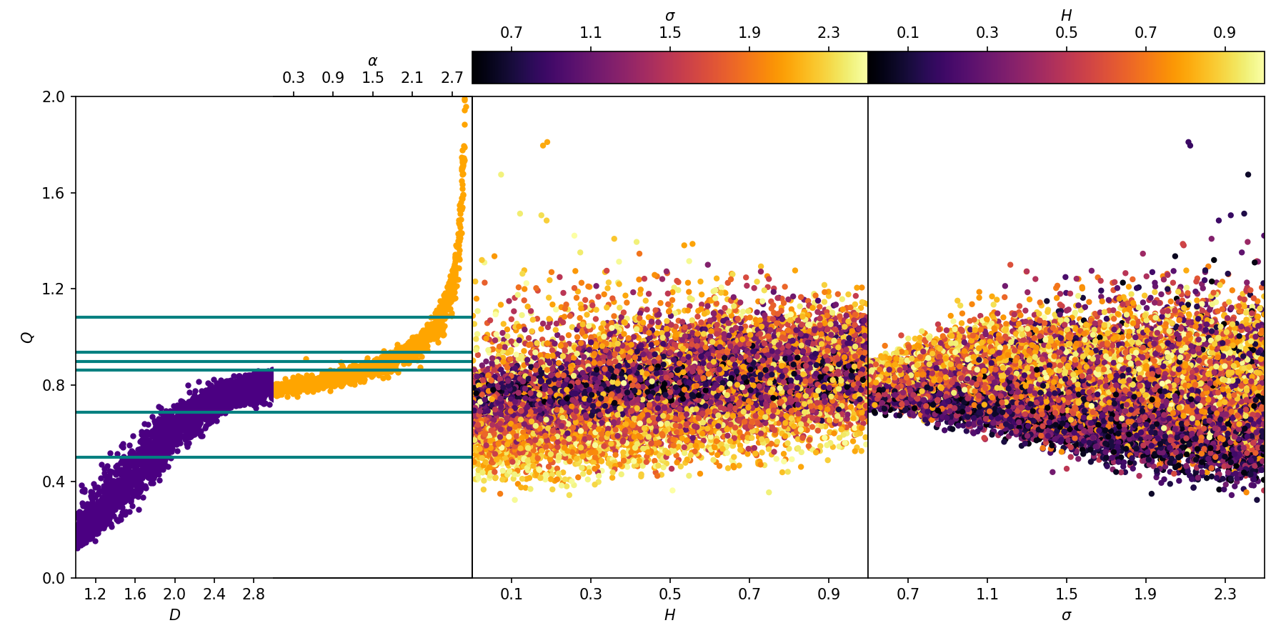
The CW04 calibration of $\mathcal{Q}$ involves calculating the statistic for BF and RDP clusters. A uniform density cluster (i.e. $D=3$ or $\alpha=0$) returns $\mathcal{Q}\sim 0.8$. BF clusters have $\mathcal{Q}\lesssim 0.8$ and RDP clusters have $\mathcal{Q}\gtrsim 0.8$. $\mathcal{Q}$ increases monotonically with both $D$ and $\alpha$. Fig. 3 shows the relationship between $\mathcal{Q}$ and $D$, and between $\mathcal{Q}$ and $\alpha$.

The $\mathcal{Q}$ values of Lupus 3, IC 348 and $\rho$ Oph suggest that they have radial density profiles with $\alpha\gtrsim 1.5$. The $\mathcal{Q}$ values of Cha I and Taurus suggest they are similar to BF structures with $D\lesssim 2.5$. The $\mathcal{Q}$ value of IC 2391 lies near a plateau on the plot, making its structural type difficult to determine.

Fig. 3 also shows how $\mathcal{Q}$ relates to the parameters of FBM clusters. Here, we see that there is a slight positive correlation between between $H$ and $\mathcal{Q}$. However, the scatter introduced by $\sigma$ exceeds the dynamic range of the correlation. There is no noticeable correlation between $\mathcal{Q}$ and $\sigma$. Therefore $\mathcal{Q}$ is a poor predictor of $H$ and/or $\sigma$.

C09 suggest that plots of $\bar{m}$ versus $\bar{s}$ provide a more robust diagnostic tool than $\mathcal{Q}$ alone. They show that BF and RDP clusters with fixed parameters fill distinct regions of the $\bar{m}$-$\bar{s}$ plot. However, there is a lack of agreement on which length scale $R$ should be used to normalise $\bar{m}$ and $\bar{s}$. In the original C09 publication, $R$ is set to the distance between the cluster’s centre of mass and its outer most point. This measure is problematic as (i) a single outlying star can dominate the length-scale and (ii) this value is not representative of the area of a cluster with a high aspect ratio. Both of these issues can add significant noise to the normalisation of $\bar{m}$ and $\bar{s}$ (see Parker, 2018, for a review of different $R$ normalisation methods). Instead, we use the Schmeja & Klessen (2006) scheme which sets $R$ to the square root of the area of the convex hull of the set of stars. This lessens (although does not necessarily eliminate) the issues with outliers and the aspect ratio.

The top frame of Fig. 4 shows how model clusters with different values of $D$ or $\alpha$ occupy different regions on the $\bar{m}$-$\bar{s}$ plot. Here, the parameter estimates for Lupus 3, IC 348 and $\rho$ Oph are unchanged from their respective $\mathcal{Q}$ estimates. In addition, the plot suggests that IC 2391 is similar to a BF cluster with $D\sim 2.8$. However, we find that Taurus and Cha I do not match up to any of the BF or RDP clusters. On visual inspection (see Fig. 2), they are clearly sub-clustered, but their $\bar{m}$-$\bar{s}$ values cannot be matched to any value of $D$.

The remaining two frames of Fig. 4 shows the $\bar{m}$-$\bar{s}$ values for FBM clusters. Here, unlike the BF and RDP models, the FBM clusters fill an area of the plot which overlaps all of the observed clusters. We see that FBM clusters with $H\sim 1$ fill the same region of the plot as RDP clusters. This is unsurprising, as they both represent smoothly distributed, centrally concentrated clusters. However, clusters with $H\lesssim 1$ do not appear to occupy distinct regions of the plot. Finally, We see a very strong negative correlation between $\bar{m}$ and $\sigma$. This shows that the mean edge-length of the minimum spanning tree is much more sensitive to the surface-density dynamic range of a cluster than its fractal properties.

$\mathcal{Q}$ and $\bar{m}$-$\bar{s}$ plots are often used to estimate underlying parameters by visual inspection. By this, we mean that a large ensemble of $\mathcal{Q}$ or $\bar{m}$-$\bar{s}$ measurements for a known set of models are plotted; parameters are attributed to an observation based on the plot-distance from the observation’s measurements to the equivalent model values. This methodology makes it difficult to quantify parameter uncertainties. Furthermore, we have shown that the BF model, which typically is used to calibrate the two methods, is unable to produce clusters with similar properties to Taurus or Cha I. The latter of these two problems may be addressed by implementing the FBM cluster model. However, the $\mathcal{Q}$ and $\bar{m}$-$\bar{s}$ methods are poor at distinguishing the underlying parameters. We address these shortcomings with a machine learning regressor which uses FBM clusters as training data.

A similar approach can be used to estimate the parameters of a star cluster. Here, $\boldsymbol{x}$ is a vector of statistics that are directly taken from the cluster (we define these in Section 3.4.1), and $\boldsymbol{y}=(H,\sigma)$ is the vector of underlying parameters. Here, the regressor $F(\boldsymbol{x})$ is an Artificial Neural Network (ANN). Complex ANNs are routinely used in fields such as image analysis (Lecun et al., 1998, e.g.). However, comparatively simple ANNs can be used for numerical regression problems with multiple inputs and outputs (Rafieferantsoa et al., 2018, e.g.).

Details of ANN used here, along with links to the full implementation in Python, are given in Appendix B. If the reader is not concerned about these technical details, they should simply note that the ANN hyperparameters are estimated from training data. Once trained, the ANN is applied to test data. This enables us to (i) ensure we are not overfitting the training data and (ii) quantify the uncertainties of the regressor. In the following sections, we discuss the training, testing and the results of the ANN.

We have shown that the BF star cluster model struggles to reproduce the observed features of substructured clusters. This because, as identified by JWL17, the BF model only produces clusters with very high surface-density variances. Therefore, we strongly suggest that the model should be retired from star cluster analysis. The FBM model presented here overcomes this problem. FBM clusters have independent parameters which (i) control the amount of fractal clustering and (ii) set the global level of surface-density variation. In addition, clusters with $H\sim 1$ fulfil the same role as centrally concentrated RDP clusters. This removes the need for using two unrelated models (i.e. BF and RDP) in the same analysis.

We find that $\mathcal{Q}$ and/or $\bar{m}$-$\bar{s}$ plot analyses are poorly suited to FBM clusters. Furthermore, they do not present robust uncertainties. This limits their efficacy, and we suggest that they should no longer be used as is. However, these analyses can be reformulated using modern machine learning techniques. Here, we present an ANN which makes robust estimates of star cluster parameters and their uncertainties. We note that alternatives to this method also exist. For example, JWL17 use principle component analysis to reduce a large range of observables to two principle features.

We have, where possible, avoided discussing these results in terms of fractal dimension. This is because $D$ does not uniquely describe a structure. For example, BF clusters with $D\sim 3$ have a roughly uniform distribution of stars. Decreasing $D$ increases the level of substructure in the distribution. Conversely, FBM clusters with $D\sim 3$ may be very substructured. Decreasing $D$ tends to fuse the sub-clumps together until the cluster is composed of one or two coherent objects. We therefore suggest caution when using the term “fractal dimension” in scientific statements. There appears to be little relation between the value of $D$ and the subjective clumpiness expressed in different models.

While the FBM model has several advantages over the BF model, there are some caveats we must address. The FBM fields generated in Section 2.1 fill a periodic box with no true centre. Here, we shift the field’s periodic centre of mass to the centre of the box. This generally places high density structures (if present) in the centre of the box, and low density regions around the edges. However, we acknowledge that this choice is arbitrary. Also, in some instances, the outline of the cluster can appear square (the effect is most pronounced when $\sigma$ is low; see Fig 2). We could address this by culling the distribution into a sphere, but this would arbitrarily remove stars from the edges of the distribution.

We have demonstrated that the ANN regressor performs well at classifying and differentiating stars clusters. However, we note that there is an infinitude of measurable features for any given cluster. We have experimented with a large number of features from different graphs (e.g. centile-based statistics, features from the Delaunay triangulation). We have found through testing that the features presented here are adequate. Adding further features to the ANN only yields very minor improvements to its estimation accuracy.

The values of $H$ and $\sigma$ are useful for categorising star clusters by their morphology. However, in order to infer physical meaning from these measures, we need to apply them to simulations. We hypothesise that, for a sub-virial substructured cluster, $\sigma$ should increase as the cluster collapses under its own gravity. Meanwhile, $H$ should increase as the collapse erases the cluster’s substructure. Conversely, for a super-viral equivalent of the same initial cluster, $\sigma$ should decrease over time as the cluster expands. It is not clear how $H$ will behave during this process. We will test these hypotheses by applying this analysis to an ensemble of $N$-body cluster simulations with various initial states.

The ANN method also provides a convenient way to compare the structure of the molecular clouds with that of star clusters. For example, Elia et al. (2014) find that molecular clouds in the galactic plane typically have $H\lesssim 0.4$, suggesting that they are similar in structure to Taurus, or Cha I. Previous numerical work has attempted to compare molecular cloud gas structure with that of embedded clusters (Lomax et al., 2011; Parker & Dale, 2015, e.g.). However, this was performed using $\mathcal{Q}$ analysis, which we have shown is unreliable. We will revisit this work and analyse the FBM properties of the stars and gas in molecular cloud simulations.

References

- André et al. (2010) André P., et al., 2010, A&A, 518, L102
- Barrado y Navascués et al. (2001) Barrado y Navascués D., Stauffer J. R., Briceño C., Patten B., Hambly N. C., Adams J. D., 2001, ApJS, 134, 103
- Bate & Bonnell (2005) Bate M. R., Bonnell I. A., 2005, MNRAS, 356, 1201
- Bontemps et al. (2001) Bontemps S., et al., 2001, A&A, 372, 173
- Cartwright (2009) Cartwright A., 2009, MNRAS, 400, 1427
- Cartwright & Whitworth (2004) Cartwright A., Whitworth A. P., 2004, MNRAS, 348, 589
- Cartwright & Whitworth (2009) Cartwright A., Whitworth A. P., 2009, MNRAS, 392, 341
- Comerón (2008) Comerón F., 2008, in Reipurth B., ed., Handbook of Star Forming Regions, Volume II. ASP Monograph Publications, p. 295
- Elia et al. (2014) Elia D., et al., 2014, ApJ, 788, 3
- Elmegreen & Falgarone (1996) Elmegreen B. G., Falgarone E., 1996, ApJ, 471, 816
- Falgarone et al. (1991) Falgarone E., Phillips T. G., Walker C. K., 1991, ApJ, 378, 186
- Federrath & Klessen (2012) Federrath C., Klessen R. S., 2012, ApJ, 761, 156
- Gaia Collaboration et al. (2016) Gaia Collaboration et al., 2016, A&A, 595, A1
- Gaia Collaboration et al. (2018) Gaia Collaboration Brown A. G. A., Vallenari A., Prusti T., de Bruijne J. H. J., Babusiaux C., Bailer-Jones C. A. L., 2018, preprint, (arXiv:1804.09365)
- Goodwin & Whitworth (2004) Goodwin S. P., Whitworth A. P., 2004, A&A, 413, 929
- Gouliermis et al. (2014) Gouliermis D. A., Hony S., Klessen R. S., 2014, MNRAS, 439, 3775
- Griffin et al. (2010) Griffin M. J., et al., 2010, A&A, 518, L3
- Jaffa et al. (2017) Jaffa S. E., Whitworth A. P., Lomax O., 2017, MNRAS, 466, 1082
- King et al. (2012) King R. R., Parker R. J., Patience J., Goodwin S. P., 2012, MNRAS, 421, 2025
- Lada et al. (2006) Lada C. J., et al., 2006, ApJ, 131, 1574
- Lecun et al. (1998) Lecun Y., Bottou L., Bengio Y., Haffner P., 1998, Proceedings of the IEEE, 86, 2278
- Lomax et al. (2011) Lomax O., Whitworth A. P., Cartwright A., 2011, MNRAS, 412, 627
- Luhman (2007) Luhman K. L., 2007, ApJS, 173, 104
- Luhman et al. (2010) Luhman K. L., Allen P. R., Espaillat C., Hartmann L., Calvet N., 2010, ApJS, 186, 111
- Molinari et al. (2010) Molinari S., et al., 2010, A&A, 518, L100
- Motte et al. (1998) Motte F., Andre P., Neri R., 1998, A&A, 336, 150
- Muench et al. (2007) Muench A. A., Lada C. J., Luhman K. L., Muzerolle J., Young E., 2007, ApJ, 134, 411
- Parker (2018) Parker R. J., 2018, MNRAS, 476, 617
- Parker & Dale (2015) Parker R. J., Dale J. E., 2015, MNRAS, 451, 3664
- Parker et al. (2014) Parker R. J., Wright N. J., Goodwin S. P., Meyer M. R., 2014, MNRAS, 438, 620
- Pedregosa et al. (2011) Pedregosa F., et al., 2011, Journal of Machine Learning Research, 12, 2825
- Peitgen & Saupe (1988) Peitgen H.-O., Saupe D., 1988, The Science of Fractal Images. Springer-Verlag
- Poglitsch et al. (2010) Poglitsch A., et al., 2010, A&A, 518, L2
- Rafieferantsoa et al. (2018) Rafieferantsoa M., Andrianomena S., Davé R., 2018, preprint, (arXiv:1803.08334)
- Schmeja & Klessen (2006) Schmeja S., Klessen R. S., 2006, A&A, 449, 151
- Schneider et al. (2013) Schneider N., et al., 2013, ApJL, 766, L17
- Smith et al. (2016) Smith R. J., Glover S. C. O., Klessen R. S., Fuller G. A., 2016, MNRAS, 455, 3640
- Steele (1988) Steele J. M., 1988, Ann. Probab., 16, 1767
- Stutzki et al. (1998) Stutzki J., Bensch F., Heithausen A., Ossenkopf V., Zielinsky M., 1998, A&A, 336, 697
- Williams et al. (2000) Williams J. P., Blitz L., McKee C. F., 2000, Protostars and Planets IV, p. 97
Acknowledgements
We thank the reviewer, Simon Goodwin, for his constructive comments. OL and APW gratefully acknowledge the support of a consolidated grant (ST/K00926/1) from the UK STFC. MLB gratefully acknowledges the support of a CDT in data intensive science (ST/P006779/1) from the UK STFC.
Appendix A Randomly sampling variates from 3 or 2 dimensional distributions
We can draw random coordinates from any gridded 3-dimensional distribution using random variates , drawn from the uniform distribution in the interval . First we calculate the cumulative distribution of along the -axis,