On the coupling of Model Predictive Control
and Robust Kalman Filtering

We briefly review the usual MPC formulation [22, Chapter 2]. We consider the discrete-time state-space model

where $x_{t}\in\mathbb{R}^{n}$, $u_{t}\in\mathbb{R}^{q}$, $y_{t}\in\mathbb{R}^{p}$, $v_{t}\in\mathbb{R}^{m}$, denote the state, the input, the output and unmeasured noise, respectively. We assume that $x_{0}$ is Gaussian distributed with mean $\bar{x}_{0}$ and covariance matrix $\bar{P}_{0}$ positive definite. For simplicity in what follows we assume that $GD^{T}=0$, that is the state noise and the observation noise are independent. Assume that our task is for the output $y_{t}$ to follow a certain reference signal $r_{t}$. To this end, we introduce the following quadratic cost function:

Here $\hat{y}_{t+k|t}$ represents the prediction of $y_{t+k}$ at time $t$ with $k>0$; $\Delta\hat{u}_{t+k|t}:=\hat{u}_{t+k|t}-\hat{u}_{t+k-1|t}$ is the predicted variation of the input from time $t+k-1$ to $t+k$ and $\textbf{u}_{t}:=[u^{T}_{t|t}\ .\ .\ .\ u^{T}_{t+H_{u}-1|t}]^{T}$. The prediction and control horizons have length $H_{p}$ and $H_{u}$, respectively, and $H_{u}\leq H_{p}$. Lastly, $Q_{k}\in\mathbb{R}^{p\times p}$ and $R_{k}\in\mathbb{R}^{q\times q}$ indicate the weight matrices for the output prediction errors at time $t+k$ and for the predicted variations of the input at time $t+k$. According to the receding horizon strategy, the control input $u_{t|t}$ to apply to $\Sigma$ at time $t$ is extracted from $\textbf{u}_{t}$ which is solution to the following open-loop optimization problem

The well known solution is, [22, Chapter 3]:

where

and $\hat{x}_{t|t}$ denotes the estimate of $x_{t}$ at time $t$. The latter is typically computed by using the Kalman filter

where the initial conditions are $\hat{x}_{0|-1}=\bar{x}_{0}$ and $P_{0}=\bar{P}_{0}$. The resulting MPC law is outlined by Algorithm 1.

Note that the estimator $\hat{x}_{t|t}$ is computed by assuming to know the actual underlying model $\Sigma$. In Section 2.2 we address the situation in which the actual model is different from $\Sigma$.

It is worth noting that the optimization problem (3) is usually considered with constraints, such as model uncertainty constraints and stability constraints. Such constraints are relatively easy to embed in (3), on the other hand the price to pay is that the corresponding problem does not admit a closed form solution. Accordingly, the computational burden of Step 4 in Algorithm 1 increases. In what follows we shall continue to consider the unconstrained MPC because, as we will see, we will embed the model uncertainty in a different way.

Assume that the actual model, denoted by $\tilde{\Sigma}$, is unknown and different from the nominal one, denoted by $\Sigma$. It is then reasonable to assume that we are able to describe this uncertainty, that is we can characterize a set of models $\mathcal{S}$ for which $\tilde{\Sigma}\in\mathcal{S}$. In the robust MPC formulation the optimization problem (3) is usually substituted by the mini-max problem [3, Section 6]:

The latter is sometimes rewritten as a constrained MPC problem. It is worth noting that solving a mini-max problem (or a constrained MPC problem) is computationally more demanding than solving a min problem. Many different uncertainty descriptions have been proposed in the literature such as impulse response uncertainty [24], structured feedback uncertainty, [15], polytopic uncertainty, [19], disturbances uncertainty, [25], probabilistic uncertainty, [9], and Gaussian processes for modeling the underlying system, [8]. Finally, in [28] it has been proposed a robust MPC wherein the cost function is an exponential-quadratic cost over the state distribution. In this way, large errors are severely penalized.

Recently, a new robust Kalman filter has been proposed [17, 35, 16, 34] which represents the generalization of the risk-sensitive filters [2, 5].

Assume that the nominal model $\Sigma$ is in the form (1), where $v_{t}\in\mathbb{R}^{m}$ is white Gaussian noise (WGN) with E[$v_{t}v^{T}_{s}$] = $\delta_{t-s}I_{m}$ ($\delta_{t}$ represents the Kronecker delta function). Moreover, the noise $v_{t}$ is independent of the initial state $x_{0}$, whose nominal distribution is given by $f_{0}(x_{0})\sim\mathcal{N}{\color[rgb]{0,0,0}(\bar{x}_{0},\bar{P}_{0})}$. We introduce the random vector $z_{t}=[\,x_{t+1}^{T}\,\ y_{t}^{T}\,]^{T}$. At time $t$ the model $\Sigma$ is completely described by the conditional probability density of $z_{t}$ given the measurements $Y_{t-1}:=[\,y_{0}^{T}\,y_{1}^{T}\,\ldots\,y_{t-1}^{T}\,]^{T}$, denoted by ${f}_{t}(z_{t}|Y_{t-1})$. Note that by construction $f_{t}(z_{t}|Y_{t-1})$ is Gaussian. Let $\tilde{f}_{t}(z_{t}|Y_{t-1})$ be the conditional probability density of the actual underlying model $\tilde{\Sigma}$ at time $t$ and assume that it is Gaussian. The discrepancy between $\tilde{\Sigma}$ and $\Sigma$ at time $t$ can be measured through the Kullback-Leibler divergence

Thus, we define as the set of all allowable models at time $t$:

that is, at time $t$ the actual model $\tilde{\Sigma}$ belongs to a ball about $\Sigma$. The radius of this ball, denoted by $c$, represents the allowable model tolerance and must be fixed a priori. Let $\mathcal{G}_{t}$ denote the class of estimators $g_{t}$ with finite second-order moments with respect to any probability density $\tilde{f}_{t}(z_{t}|Y_{t-1})\in\mathcal{S}_{t}$.

We define as robust estimator of $x_{t+1}$ given $Y_{t}$ the solution to the following mini-max problem

where

is the mean square error of the estimator with respect to the actual model $\tilde{\Sigma}$. Finally, the robust estimator of $x_{t}$ given $Y_{t}$, i.e. $\hat{x}_{t|t}$, is defined as the minimum mean square error based on (1) propagating $\tilde{f}_{t}(z_{t}|Y_{t-1})$.

In [17] the solution of the mini-max problem (12) is characterized in the context of systems without inputs. However the generalisation of this result to the more general case of feedback control systems is not trivial and needs to be properly addressed. In the following theorem we consider a system with an input composed of a deterministic part plus a linear combination of the past values of the output, see Equation (4), and we show that the robust filter (12) still obeys to a Kalman-like recursion.

The choice of the tolerance parameter $c$ is a delicate step. In the design phase, the user typically has: (i) an accurate and complex model of the actual process; in practice this model can be understood as an exact description of the actual process so that $\tilde{\Sigma}$ is known and coincides with this model; (ii) a simple model $\Sigma$ of the actual process of the form (1). Since $\tilde{\Sigma}$ and $\Sigma$ are known, then we can compute $\mathcal{D}(\tilde{f}_{t},f_{t})$ defined in (10). Therefore, as an initial guess the parameter $c$ can be chosen as the average of $\mathcal{D}(\tilde{f}_{t},f_{t})$ over the interval of interest $t=1\ldots t_{MAX}$.

The constraint $\tilde{f}_{t}\in\mathcal{S}_{t}$, i.e. $\mathcal{D}(\tilde{f}_{t},f_{t})\leq c$, in (12) can be made soft by adding a penalty term in the objective function

where $\mathcal{V}_{t}:=\{\tilde{f}_{t}(z_{t}|Y_{t-1})\ |\ \mathcal{D}(\tilde{f}_{t},{f}_{t})\leq\infty\}$ and $\bar{\theta}>0$ is fixed a priori. It is worth noting that the solution to (17) is the risk-sensitive filter with risk sensitivity parameter $\bar{\theta}$, see [5].

To recap, in the presence of an input $u_{t}=a_{t}(Y_{t})+b_{t}(r_{t})$ we have modified the robust Kalman filter and the risk-sensitive filter by adding the term $Bu_{t}$ in (6). Even if the modification is very intuitive, it is not straightforward the fact that the modified filters are still robust (in the precise sense of [5] and [17], respectively). Theorem 1 and Theorem 2 showed that robustness is preserved in this case.

The robust MPC law that we propose is constituted by two steps: first, we compute a robust estimate of $x_{t}$ given $Y_{t}$ according to (12); second, the optimal input control $u_{t|t}$ is computed as in (4). Since $u_{t|t}$ is a function of $\{\mathbf{r}_{t},\hat{x}_{t|t}\}$ and thus a function of $\{\mathbf{r}_{t},Y_{t}\}$, Theorem 1 holds and the robust filter (12) obeys to a Kalman-like recursion. The resulting robust MPC law is outlined in Algorithm 3.

To avoid the computation of $\theta_{t}$ in Step 2, we can approximate this robust filter with the risk-sensitive filter in Theorem 2. More precisely, since we know that $\theta_{t}\rightarrow\bar{\theta}$ as $t\rightarrow\infty$, we can approximate it with the risk-sensitive filter (17) with risk sensitivity parameter equal to $\bar{\theta}$.

We now present the complete model including the nonlinear dynamics, that will represent the actual model in our simulations. The equations describing the physics of the system are:

where $\theta_{\ell}$ denotes the load angle; $\theta_{m}$ the motor angle; $T_{m}$ the torque generated by the motor; $E_{m}$ the back electromotive force; $V$ the motor armature voltage; $I_{m}$ the armature current; $T_{s}$ the torsional torque; $J_{\ell}$ the load inertia. Moreover $T_{f_{\ell}}(\dot{\theta}_{\ell})$ and $T_{f_{m}}(\dot{\theta}_{m})$ represent the Coulomb and the deadzone frictions on the load and on the motor, as described in detail in [14]:

where the function $\operatorname{sgn}$ is defined as:

The profile of the nonlinear friction model is depicted in Fig. 2

The nominal values of the parameters of the servomechanism system are reported in Tab. 4.1. In practice, these values are not accurate because they are difficult to estimate. Accordingly, we introduce two kinds of possible parameter perturbations, $\varepsilon_{min}$ and $\varepsilon_{max}$, expressing the percentage of the relative error that each nominal value can be affected by. In the actual model every nominal parameter is perturbed in this way: if the nominal value is considered reliable enough it is perturbed by $\pm\varepsilon_{min}=\pm 5\%$, otherwise by $\pm\varepsilon_{max}=\pm 10\%$, see Tab.4.1.

We now derive the nominal model. To obtain a linearized model of the servomechanism system we eliminate the nonlinear dynamics (20)-(21) and set $L=0$. The dynamic equations resulting from these simplifications are:

wherein we consider the nominal parameters in Tab. 4.1. Defining as state vector $x_{t}=[\,\theta_{\ell}\ \ \dot{\theta}_{\ell}\ \ \theta_{m}\ \ \dot{\theta}_{m}\,]^{T}$, we obtain a continuous-time state-space linear model of type

where $u_{t}$ is the motor armature voltage, $y_{t}$ the load angle, $w_{t}$ is the normalized Wiener process, and matrices $\bar{G}$, $\bar{D}$ are chosen heuristically in such a way to compensate the approximations made before. Lastly this model was discretized with sampling time $T=0.1$ s obtaining in this way a model of type (1).

In this section we want to show the improvement in performance brought by the MPC controller equipped with the robust Kalman filter in Theorem 1 (R-MPC). As terms of comparison we consider two other controllers: standard MPC (S-MPC) and MPC equipped with the risk-sensitive filter in Theorem 2 (RS-MPC).

More specifically we study their performances in response with the reference trajectory set to $r_{t}=\pi/2$ rad, $t\geq 0$ with $y_{0}=0$ rad. The initial state $x_{0}$ is assumed to be zero mean and with variance equal to the variance of the state-process noise in (1). Regarding the parameters of MPC in the cost function (2) we consider the weight matrices $Q_{k}=0.1$, $R_{k}=0.1$ and $H_{p}=10$, $H_{u}=3$. In particular the effects of the choice of $H_{p}$ and $H_{u}$ are further analyzed in the last simulation, see Fig.8.

In the first simulation we consider the ideal situation in which the actual model coincides with the one of Section 4.2, that is the actual and the nominal models coincide. As can be seen in Fig.3,

S-MPC can track the reference trajectory likewise R-MPC (with $c=10^{-1}$). However, it is worth noting that the input applied by R-MPC is less smooth, see Fig. 4.

This is not a very surprising fact given that the robust filter is constructed under the idea of considering more uncertainties in the modelling. The performance of RS-MPC has been omitted because similar to the one of R-MPC.

In the second simulation, the actual model is the one of Section 4.1. Fig. 5

shows the load angle for S-MPC, R-MPC (with $c=10^{-1}$) and RS-MPC (with $\bar{\theta}$ set to the value at steady state computed through R-MPC).

The differences between the three controllers are clearly visible. In particular it is evident how R-MPC is able to provide an adequate control whereas RS-MPC and S-MPC do not. To give a quantitative analysis, in the first simulation we can see how after 5 seconds the error on the output is comprised within 5% of the desired trajectory for all the controls (i.e. S-MPC, RS-MPC and R-MPC). On the other hand, in the second simulation the error on the output is comprised within 5% of the desired trajectory after 8 seconds for R-MPC, after 19 seconds for RS-MPC and the one of S-MPC never reaches this accuracy in 35 seconds. Again, R-MPC is the unique control providing similar performances both in the first and in the second simulation. On the other hand, R-MPC requires more energy (see Fig. 6 on the interval 3$\div$10 seconds) than S-MPC. Finally, RS-MPC constitutes an in-between solution in terms of performance.

The third simulation has the aim to evaluate the effect of the tolerance $c$ on the performance of R-MPC, see Fig. 7. More precisely we consider R-MPC1 with $c=10^{-1}$, R-MPC2 with $c=10^{-2}$, and R-MPC3 with $c=10^{-3}$. We consider a Monte Carlo experiment of 200 runs. At each run we generate the actual model where $\varepsilon_{min}$ and $\varepsilon_{max}$ in Tab. 4.1 are randomly chosen inside the interval, respectively, [-10%,10%] and [-20%,20%] following a uniform distribution probability. The unique exception is for the load inertia $J_{\ell}$ which is perturbed randomly with a relative error uniformly distributed inside the interval [-80%,80%]. In this way we consider the situation in which the servomechanism system is connected to different loads during its operational life. Then, we apply the MPC controls and for each of them we compute the MSE of the output with respect to the reference signal during the first 20 seconds (in which the control with R-MPC usually approaches the steady state, as seen in Fig.5).

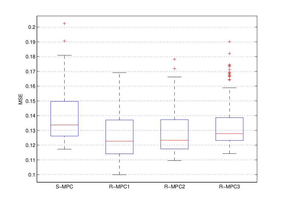
As expected, R-MPC performs more accurately than S-MPC and, interestingly enough, higher values of $c$ correspond to a diminished error of the MSE of R-MPC. On the other hand, higher values of $c$ correspond to high-energy control inputs.

As a last simulation, we analyze the influence of the length of the prediction and control horizons on the performance. To this aim, we have carried out the third simulation for different choices of the horizons. As representative examples, in Fig. 8 we report the results corresponding to $H_{p}=10,H_{u}=8$ and $H_{p}=15,H_{u}=3$. The first case shows that a large value for the control horizon significantly reduces the tracking error for all the MPC controllers. In particular, R-MPC1 provides the best performance while S-MPC provides the worst one. Conversely, a large value for the prediction horizon (second case) is detrimental to the performance of the MPC controllers. In particular, all the MPC controllers perform in a similar way and R-MPC3 is slightly better than the others. Finally, we have noticed that the control action is very responsive with $H_{u}$ large and very slow with $H_{p}$ large.

To prove the statement we need the following result, see [34, 16].

In view of Lemma 1, it is worth noting that the estimation error $e:=x-g(y)$ under the least favorable model is Gaussian and with zero mean and covariance matrix $V$.

We now proceed to prove the statement. Assume that the statement holds at time $t$, that is the robust estimator of $x_{t}$ given $Y_{t-1}$ is $\hat{x}_{t|t-1}=\mathbb{E}_{\tilde{f}_{t}}[x_{t}|Y_{t-1}]$ and the prediction error $e_{t}=x_{t}-\hat{x}_{t|t-1}$ is Gaussian with zero mean and covariance matrix $V_{t}$. We consider now the nominal model (1). Since $a_{t}(Y_{t})$ is a linear function, we have

References

- [1] Peyman Bagheri, Peyman Bagheri Ali, Ali Khaki Sedigh, and Khaki Sedigh. Analytical approach to tuning of model predictive control for first-order plus dead time models. IET Control Theory & Applications, 7(14):1806–1817, 2013.
- [2] R. N. Banavar and J. L. Speyer. Properties of risk-sensitive filters/estimators. IEEE Proceedings - Control Theory and Applications, 145(1):106–112, Jan 1998.
- [3] A. Bemporad and M. Morari. Robust model predictive control: a survey. Lecture Notes in Control and Information Sciences, 245:207–226, 2007.
- [4] A. Bemporad and E. Mosca. Fulfilling hard constraints in uncertain linear systems by reference managing. Automatica, 34(4):451–461, 1998.
- [5] R. K. Boel, M. R. James, and I. R. Petersen. Robustness and risk-sensitive filtering. IEEE Transactions on Automatic Control, 47(3):451–461, 2002.
- [6] G. C. Calafiore and L. Fagiano. Robust model predictive control via scenario optimization. IEEE Transactions on Automatic Control, 58(1):219–224, Jan 2013.
- [7] E. F. Camacho and C. Bordons. Model predictive control in the process industry. Springer Science & Business Media, 2012.
- [8] Gang Cao, Edmund M-K Lai, and Fakhrul Alam. Gaussian process model predictive control of unknown non-linear systems. IET Control Theory & Applications, 11(5):703–713, 2017.
- [9] D. Chatterjee, P. Hokayem, and J. Lygeros. Stochastic receding horizon control with bounded control inputs: A vector space approach. IEEE Transactions on Automatic Control, 56(11):2704–2710, Nov 2011.
- [10] L. Hansen and T. Sargent. Recursive robust estimation and control without commitment. Journal of Economic Theory, 136(1):1–27, 2007.
- [11] L. Hansen and T. Sargent. Robustness. Princeton University Press, Princeton, NJ, 2008.
- [12] B. Hassibi, A. Sayed, and T. Kailath. Indefinite-Quadratic Estimation and Control– A Unified Approach to and Theories. Soc. Indust. Appl. Math., Philadelphia, 1999.
- [13] A. A. Jalali and V. Nadimi. A survey on robust model predictive control from 1999-2006. In Internation Conference on Computational Intelligence for Modelling Control and Automation and International Conference on Intelligent Agents, Web Technologies and Internet Commerce, 2006.
- [14] T. Kara and I. Eker. Nonlinear modeling and identification of a {DC} motor for bidirectional operation with real time experiments. Energy Conversion and Management, 45(7-8):1087 – 1106, 2004.
- [15] M. V. Kothare, V. Balakrishnan, and M. Morari. Robust constrained model predictive control using linear matrix inequalities. Automatica, 32(10):1361 – 1379, 1996.
- [16] B. C. Levy and R. Nikoukhah. Robust least-squares estimation with a relative entropy constraint. IEEE Transactions on Information Theory, 50(1):89–104, Jan 2004.
- [17] B. C. Levy and R. Nikoukhah. Robust state space filtering under incremental model perturbations subject to a relative entropy tolerance. IEEE Transactions on Automatic Control, 58(3):682–695, March 2013.
- [18] B. C. Levy and M. Zorzi. A contraction analysis of the convergence of risk-sensitive filters. SIAM J. Optimization Control, 54(4):2154–2173, 2016.
- [19] Shuai Liu, Yan Song, Guoliang Wei, and Xuegang Huang. Rmpc-based security problem for polytopic uncertain system subject to deception attacks and persistent disturbances. IET Control Theory & Applications, 11(10):1611–1618, 2017.
- [20] Yong-Hua Liu. Saturated robust adaptive control for uncertain non-linear systems using a new approximate model. IET Control Theory & Applications, 11(6):870–876, 2017.
- [21] J. Maciejowski. Discussion on: âmin-max model predictive control of nonlinear systems: A unifying overview on stability”. European Journal of Control, 15(1):22–25, 2009.
- [22] J. M. Maciejowski. Predictive control: with constraints. Pearson education, 2001.
- [23] D. Q. Mayne. Model predictive control: Recent developments and future promise. Automatica, 50(12):2967 – 2986, 2014.
- [24] G. De Nicolao, L. Magni, and R. Scattolini. Robust predictive control of systems with uncertain impulse response. Automatica, 32(10):1475–1479, 1996.
- [25] P. E. Orukpe and I. M. Jaimoukha. Robust model predictive control based on mixed control approach. Proceedings of the European Conference, pages 2223–2228, August 2009.
- [26] S. J. Qin and T. A. Badgwell. A survey of industrial model predictive control technology. Control Engineering Practice II, pages 733–764, 2003.
- [27] Ting Shi and Hongye Su. Sampled-data mpc for lpv systems with input saturation. IET Control Theory & Applications, 8(17):1781–1788, 2014.
- [28] X. Yang and J. Maciejowski. Risk-sensitive model predictive control with gaussian process models. IFAC-PapersOnLine, 48(28):374–379, 2015.
- [29] M. Yoon, V. Ugrinovskii, and I. Petersen. Robust finite horizon minimax filtering for discrete-time stochastic uncertain systems. Syst. Control Lett., 52:99–112, 2004.
- [30] Langwen Zhang, Jingcheng Wang, Yang Ge, and Bohui Wang. Robust distributed model predictive control for uncertain networked control systems. IET Control Theory & Applications, 8(17):1843–1851, 2014.
- [31] M. Zorzi. A new family of high-resolution multivariate spectral estimators. IEEE Trans. Autom. Control, 59(4):892–904, Apr. 2014.
- [32] M. Zorzi. An interpretation of the dual problem of the THREE-like approaches. Automatica, 62:87–92, 2015.
- [33] M. Zorzi. Multivariate spectral estimation based on the concept of optimal prediction. IEEE Transactions on Automatic Control, 60(6):1647–1652, June 2015.
- [34] M. Zorzi. On the robustness of the Bayes and Wiener estimators under model uncertainty. Automatica, 83:133–140, 2017.
- [35] M. Zorzi. Robust Kalman filtering under model perturbations. IEEE Transactions on Automatic Control, 62:2902–2907, Jun 2017.
- [36] M. Zorzi and B. C. Levy. On the convergence of a risk sensitive like filter. In 54th IEEE Conference on Decision and Control, Osaka,Japan, December 2015.
- [37] Mattia Zorzi. Convergence analysis of a family of robust kalman filters based on the contraction principle. SIAM Journal on Optimization and Control, 55(5):3116–3131, 2017.
6 Appendix
6.1 Proof of Theorem 1
Lemma 1.
Let be a random vector with nominal and actual probability density, respectively, and . We conformably partition the mean and the covariance of :
and likewise for and . Consider the mini-max problem