Is a Finite Intersection of Balls Covered by
a Finite Union of Balls in Euclidean Spaces ?
Abstract
Considering a finite intersection of balls and a finite union of other balls in an Euclidean space, we propose an exact method to test whether the intersection is covered by the union. We reformulate this problem into quadratic programming problems. For each problem, we study the intersection between a sphere and a Voronoi-like polyhedron. That way we get information about a possible overlap between the frontier of the union and the intersection of balls. If the polyhedra are non-degenerate, the initial nonconvex geometric problem, which is NP-hard in general, is tractable in polynomial time by convex optimization tools and vertex enumeration. Under some mild conditions the vertex enumeration can be skipped. Simulations highlight the accuracy and efficiency of our approach compared with competing algorithms in Python for nonconvex quadratically constrained quadratic programming. This work is motivated by an application in statistics to the problem of multidimensional changepoint detection using pruned dynamic programming algorithms.
Nonconvex quadratically constrained quadratic programming, ball covering problem, computational geometry, Voronoi-like polyhedron, vertex enumeration, polynomial time complexity.
MS classification : 90C26, 52C17, 68U05, 62L10.
1 Introduction
1.1 Problem description
We consider two finite sets of balls in an Euclidean space, and , with and arbitrary centers and radii. We introduce the intersection set and union set . Our problem consists in finding an exact and efficient method to decide whether the inclusion is true or false.
Denoting by the complement of , this problem is equivalent to the study of the emptiness of which is a challenging question, both theoretically and computationally due to the non-convexity of the sets ().
With the -dimensional Euclidean space, , the open balls and closed balls are defined by their centers and radii respectively. Thus
where , with , is the Euclidean norm. We assume that the centers of balls in are all different (non-concentric) and that for all and (with and ) we have:
| (1.1) |
These conditions can be verified in polynomial time in a preprocessing step in order to avoid unnecessary computations (for example, we remove in if ) or trivial solutions (for example, if , then ).
Remark 1.1.
We consider open balls . This is useful in proofs because we get the set open. With closed balls the decision problem is the same.
We reformulate our geometric problem into a collection of quadratically constrained quadratic programming (QCQP) : for ,
| (1.2) |
We solve these problems sequentially for increasing integers . Notwithstanding the difficult resolution of (1.2), the naive Algorithm 1 gives an exact response concerning the geometric inclusion .
The feasible region is the subset of points in satisfying the constraints in problem . If the (nonempty) feasible region for problem is strictly included into , that is, for all , then and covers . Thus, Algorithm 1 tries to cover with the balls in , adding them one by one. The algorithm stops as soon as the feasible region becomes empty (justifying the while loop).
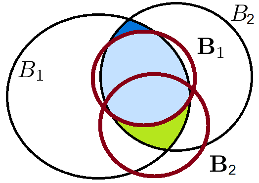
Other reformulations are possible. We choose one of them ensuring the feasibility of the considered problem at each step . If feasibility is not required, solving is enougth work. In both cases, the non-convexity of the initial geometric problem is transferred to problems for which the feasible regions (if and ) and the objective functions (with the standard formulation with a minimization) are nonconvex. For this reason, line search strategies for interior point methods can fail to converge towards the global optimum. On a simple example in Figure 1 we highlight the failing of any point following methods.
For decades, many approximate methods for the generic nonconvex QCQP problems (1.2) have been developed (see the review [23]) to avoid using primal methods. They are relaxation methods that usually convexify the nonconvex part of the problem or solve successive convex optimization approximate problems. Approaches as semi-definite relaxation (SDR)[24], reformulation linearization technique (RLT)[18] or successive convex approximation (SCA)[21, 26] are among the most popular. However, they are often computationally greedy (using unknowns) and only converge towards KKT stationary points.
We propose in this paper, to the best of our knowledge, the first exact and simple problem-solving method for the subclass of nonconvex QCQP problems involving only balls and complement of balls.
1.2 Proposed solution
Our QCQP problem is specific as it only involves balls. We can take advantage of the fact that the intersection of two spheres, when they meet, belongs to an hyperplane, which is both concave and convex. Considering a sphere , where denotes the frontier operator, we build hyperplanes as soon as a sphere or intersects . Each hyperplane defines a favored half-space. The intersection of the obtained half-spaces yields an open convex polyhedron which can be seen as a Voronoi-like structure.
We introduce the notation and prove that we are able to detect an intersection between and only by using the convex polyhedron . This method is based on the set equality . The closure of is denoted . Detection of a nonempty intersection can be handled solving the following ( for the minimum and for the maximum) quadratic programs (QP): for ,
| (1.3) |
The minimum QP problem is tractable in polynomial time [17, 27]. Solving for the maximum is a nonconvex (concave) problem, which can be solved by vertex enumeration in polynomial time if the polyhedron is non-degenerate [4]. There exists particuliar cases, in practice rarely encountered, for which the vertex enumeration problem remains NP-hard [13].
In fact, as soon as we find a feasible point strictly inside the ball and another one striclty outside, we have and we will prove that .
If for all , this intersection is empty, we have for all , that is . Thus, with our method we shift from the emptiness of set to the emptiness of set . To solve the initial covering problem ( ?), we notice that we only need to know a point inside and test whether this point is also inside to decide our question.
1.3 Outline
Section 2 presents in detail the proposed solution. In particular, we show that the non-feasibility of Problem gives also information on the initial geometric structure. In Appendix A we propose a similar method adapted to covering tests for large or sequential tests.
With some conditions on the centers and radii of the balls in , we are able to ensure that the polyhedron is unbounded and can then skip the maximization problem to only consider the convex quadratic one. We present in Section 3 several cases where the only problem to solve is convex. If , we introduce the so-called concave QCQP problem and highlight simplified results.
Finally, in Section 4, we compare our approach with recent methods of the Python library ’qcqp’ gathering together the best approaches for solving nonconvex QCQP. These simulations highlight the benefit of our method specifically developed for the problem at hand.
This work is motivated by an application to a changepoint detection method in statistics as explained in next Subsection 1.4. This introductory section ends with a bibliographical review.
1.4 Motivation
Our covering problem has a direct application for the implementation of the pruned penalized11 1 It would also work for (non penalized) segment neighborhood method [2]. dynamic programming algorithm for changepoint detection in a multidimensional setting [12, 20, 25]. This problem consists in finding the optimal changepoint within the set such that we minimize a quadratic (for Gaussian modelization) penalized cost (by ):
and the data to segment. Using a dynamic programming procedure, we build the recursion with and the initialization . We solve this recursion iteratively from to .
At each , the recursive function is a piecewise quadratic function defined on non-overlapping regions , for which each quadratics is active on a set of type ””. Precisely,
where all the ”” sets designate balls determined by the data . At the next iteration , each is intersected by a new ball (that is, we add a ball in each ) and the set is created.
In order to get the global minimum we compare the minima of all present quadratics. To speed-up the procedure, it is worthwhile to search for vanishing sets, that is to detect efficiently the emptiness of sets . In fact, once a set is proved to be empty, we do not need to consider its minimum anymore at any further iteration. This method is called pruning in the changepoint detection literature.
In a paper in preparation, we will compare this exact method to heuristic approaches in order to build a fast algorithm for an application to genomic data. Morever, our methods can be extended to other distributions of the natural exponential family.
1.5 Bibliographical review
Geometric problems for balls often separately address the intersection and the union problems. Without optimization tools, the detection of a nonempty intersection between balls is difficult to solve. Helly-type theorems can be adapted to balls [5, 19] but no efficient algorithm arises from this approach. The union of balls is a problem linked in the literature to molecular structures, where the volume and the surface area of molecules in 3D are important properties. Powerful algorithms based on Voronoi diagrams have been recently developed [3, 8]. Even if the number of balls is small, that is more than two, the exact computation of simple geometric properties as volume are challenging questions [9].
One of the first problems to associate union and intersection is the historical disk covering problem, which consists in finding the minimum number of identical disks (with a given radius) needed to cover the unit disk [6]. This problem is still open and remains mainly unsolved, although research on this subject is active [1, 10] as it has pratical applications, for example in optical interferometry [22].
Our problem also involves covers but is different in several important ways. Indeed, we study the covering of an intersection of balls by other balls which are not necessary of the same size. Furthermore, we do not consider the question of the optimal covering, but only the covering test. This problem is part of computational geometry problems and, as far as we know, is original in the literature. Our reformulation in a QP problem plays a central role as it allows the building of an exact and efficient decision test.
Nonconvex QCQP problems are a major issue for many practical applications: problems of transmit beamforming in wireless communication [15] or signal processing [16] have stimulated the development of this research area. The problem we consider in this paper is another example of a problem driven by application.
2 Equivalent quadratic programming
We first focus on the building of a unique polyhedron and show its close link with the initial nonconvex sets . Finally, we show that the polyhedra and their associated quadratic programs solve the problem.
2.1 Linear constraints
From now one, we consider a unique problem centered on the closed ball and write , , , , , . For all such that and intersect, we have the hyperplane equation given by
| (2.1) |
and the open half-space containing the set : .
The geometric configuration of the balls and with the half-space is given on Figure 2 (left). All the balls in intersect and the inclusion is not excluded (see conditions (1.1)): in this case, we do not build any hyperplane.
Similar hyperplanes and half-spaces are built between spheres and for when they intersect, but here, we consider the half-space containing . Therefore,
and .
If , a case not excluded in (1.1), we also do not build hyperplane.

With these half-spaces, we define the open convex polyhedron
and the polyhedra and such that . The open polyhedron will be used to prove geometrical properties, whereas its closure is the feasible region of the QP problem .
An efficient resolution of the nonconvex problem of type (cf (1.3)) for maximum is made possible, solving for example a vertex enumeration problem [4]. An example of feasible region is drawn on Figure 2 (right).
Before proving the equivalence of Problems (1.2) and (1.3), we present some simple equalities and inclusions used throughout this paper between sets involving balls and hyperplanes.
Lemma 2.1.
For and , we have the relations:
The proof is straightforward.
2.2 Links between the polyhedron and the initial geometric problem
We give a set equality linking the convex polyhedron and the open set involved in the initial geometric problem.
Corollary 2.1.
.
Proof.
This corollary is a central result. The following proposition is a technical topological result used in the next subsection.
For , we introduce the ball with center and radius . We also define . is the volume (Lebesgue measure) in dimension . In the following proposition, we connect the position of points in the closed feasible region to the spatial position of .
Proposition 2.1.
If the volume of the feasible region is nonzero (), the following assertions are equivalent:
i) ,
ii) there exists such that ,
iii) (the Lebesgue measure of the surface area is nonzero),
iv) there exists such that for all , .
To state this result, we use the following lemma.
Lemma 2.2.
With an open set of , we have equivalence between propositions:
a) ;
b) ;
c) there exists such that for all , .
Proof.
With , there exists an open ball centered on and of radius such that . Thus and for all , . We have shown that . The implication is obvious and the Lemma is proven. ∎
Proof of Proposition 2.1.
The implication is due to the openness of . We prove the converse. As and is convex, we have and . Thus, there exist sequences and such that and with for all . Therefore, there exists such that, for all , . By convexity of , we get . We use the Lemma 2.2 () with the open set to prove the equivalence between and , knowing that . As (see Corollary 2.1), we use again Lemma 2.2 () with the open set to get the equivalence between propositions and . ∎
With this last result, we have shown that some propositions involving the closed polyhedron are related to results using and hence . We now combine this result with the quadratic programming problem to solve the problem.
2.3 Quadratic programming decision
We still focus on a unique quadratic program:
| (2.2) |
and we denote by (resp. ) the value of the argument for which the objective function attains its minimum (resp. maximum) over the set . Notice that, if is unbounded, and in some singular cases, the argument of the maximum may not be unique.
The non-existence of a point or satisfying the strict inequalities in Proposition 2.1 case (i) is related to the resolution of problem . For example, there is no point if . Before solving this extremum problem, one should verify the feasibility of the constraints. Studying the feasibility of these constraints, we get some inclusion criteria.
Proposition 2.2.
If , then (or ),
if , then ,
if , then .
Proof.
We can now present our main result, showing the equivalent between the resolution of the QP problems , , and the decision about .
Theorem 2.1.
(A) If there exists such that , then , and ;
(B) if or , then .
Proof.
In case (A), Proposition 2.1 gives the existence of and such that . In particular, , then . Consequently, (an open set) and . With a point we get and . Case (B) is the negation of case (A). That is, there exists such that for all or for all , we have using Proposition 2.1. Therefore . Otherwise, with in Lemma 2.2 we get for all and fixed , which is impossible. ∎
If case (B) is satisfied, the convex set does not intersect the frontier and we consider another reference ball in to solve a new -type problem (1.3). If for all elements of we get case (B), we have . Using a point in , we test whether is included in to conclude.
3 Simplifications
3.1 Convex reduction
We show that if some mild conditions are satisfied, the feasible region of Problem (see (2.2)) can be unbounded and the maximum problem in Theorem 2.1 does not have to be solved anymore (). The problem is reduced to a convex quadratic programming problem which can be solved in polynomial time [17, 27].
Theorem 3.1.
For all and , if and , then or .
Proof.
First, we show that . Indeed, we have for ,
and for ,
using the hypothesis. Second, we prove that, if , then is unbounded. Suppose that there exists . We consider the linear functions and with . We have , and , , so that these functions are strictly increasing. Thus, for all negative lambda, we have . Therefore, as , the set can not be empty. ∎
With only an upper bound on the number of involved balls in , we have the same result.
Proposition 3.1.
If the number of constraints is less or equal to the dimension, that is , then is unbounded (or empty) and the conclusion of Theorem 3.1 still holds.
Proof.
We explicit the constraints as a system of linear inequalities, , with and . If is nonsingular, the system with the vector filled by ones, has a (unique) solution and with . If is singular, the rank-nullity theorem shows that the linear subspace is of dimension and then . If a point satisfies the inequalities, thus, with and . We have and the result is proven. ∎
Remark 3.1.
The conditions of Lemma 3.1 are sharp. If one of the relations is false, then there exist sets of balls and with , such that we have . An example of such a set is the -dimensional pyramid with summit near point and a basis obtained with the only one hyperplane that do not satisfies the conditions of the theorem. The necessary condition of Proposition 3.1 is verified as .
Theorem 3.2.
If there exists such that and for all and (linear separability) then is unbounded or .
Proof.
Suppose that there exists and satisfying the condition of the theorem. Then for all , we have for all the constraints
and definies an infinite direction inside the polyhedron . ∎
3.2 The concave QCQP problem
If there is only one ball in the set and then no more concave constraint in (1.2), we consider only one QCQP problem of type (1.2) and only one QP problem of type (2.2) (). We say that we solve a concave QCQP problem because we minimize the opposite of a convex function over a set of convex constraints.
A first direct consequence is that , and . In this particular configuration, some of our results in Section 2 and Subsection 3.1 can be simplified.
Feasibility:
If , then (or ).
Quadratic programming reduction:
(A) If is such that , then ;
(B) if , then ;
(C) if then .
Proof.
Only the case (C) has to be proven. using Lemma 2.1. However, and then . ∎
Convex optimization reduction:
if , for all , then or .
4 Simulations
Algorithm 2 describes our new procedure based on equivalent QP problems. It is made of two steps: the detection of an intersection between and using QP problems (see Section 2) and the test with a unique point (if ). We chose to determine and for each QP problem but in fact we only need points and as shown by Theorem 2.1.
Our goal is to compare the performances of this algorithm against Algorithm 1 on two aspects: the exactness of the result and their computational efficiency. We will also illustrate the polynomial time complexity of our new algorithm by increasing the dimension at fixed and .
We have implemented22 2 The Python code is available on my github ’vrunge’ in repository called ’QP_vs_QCQP’ https://github.com/vrunge/QP_vs_QCQP/blob/master/simulations.ipynb the Algorithm 1 in Python using the recent (2017) suggest and improve method for nonconvex QCQP [23] based on packages ’cvxpy’ [11] and its extension ’qcqp’. This allows us to use state-of-the-art methods on Python, more elaborated than interior point one, which is not adapted to our problem (see Figure 1). The suggest method is set to random and the improve step to ADMM (alternating directions method of multipliers [7]) followed by a coordinate descent step. This is the most efficient combinaison of methods (empirically speaking) and is used in some examples given in the package.
The center points for balls are randomly generated with a normal distribution centered on zero with standard deviation and their radius is the distance to zero plus a quantity for intersection ball and for union balls. We also verify that the obtained balls intersect each other as in (1.1), if not, we simulate new balls. Examples of simulated data are shown in Figure 3.
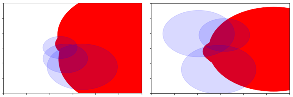
In Table 1, we generate 100 examples for each proposed configuration. We first consider examples with . In case we compare the results of the two algorithms with the 2d graphical representation of the balls problem to confirm the exactness of our method.
Algorithm 2 always finds the exact result in dimension and we get the value . For higher dimensions, we know the result of Algorithm 2 to be exact (as shown by theoretical results of Section 2) and count the number of identical results between the two algorithms to get the number of true results for Algorithm 1. Algorithm 1 often fails, in particular when the non inclusion is difficult to visually detect (obtained on a small volume). This behavior is a consequence of our simulations: we generated data with a unique simulation procedure, so that, for increasing it becomes harder to generate examples without inclusion. An increasing dimension gives more space to get a non inclusion and facilitate the detection of for Algorithm 1.
In the case of the inclusion , we notice that Algorithm 1 always finds the right answer in our simulations. Interestingly, the resolution of the unique problem often fails, unlike the non inclusion case.
| , | , | , | |||||
| Algorithm 1 | 83 | 65 | 48 | 57 | 63 | 79 | 65 |
| 83 | 80 | 87 | 91 | 91 | 90 | 92 | |
| Algorithm 2 | 100 | 100 | 100 | ||||
| Algorithm 1 | 100 | 100 | 100 | 100 | 100 | 100 | 100 |
| 100 | 92 | 81 | 75 | 75 | 83 | 77 | |
In Table 2 we highlight the efficiency of our new algorithm compared with the Python package ’qcqp’ based on nonconvex QCQP methods. Notice that improvements in the code for Algorithm 2 are still possible with a direct implementation of the QP problem stopping as soon as we get or and in the vertex enumeration solver (we simply used package cdd33 3 website of the Python package http://pycddlib.readthedocs.io/en/latest/[14]). We have made simulations () for configurations () with in case (simplier to obtain in our ball generation algorithm with increasing dimension ). Our results show for the Algorithm 1 a computational time complexity of order slower than for Algorithm 2 and a higher time variability between iterates.
| i | time QP | time QCQP | time QP | time QCQP | time QP | time QCQP |
|---|---|---|---|---|---|---|
| 1 | 0.00411 | 2.013 | 0.00448 | 2.667 | 0.00464 | 2.923 |
| 2 | 0.00280 | 1.213 | 0.00261 | 2.553 | 0.00298 | 1.732 |
| 3 | 0.00260 | 1.034 | 0.00262 | 2.358 | 0.00305 | 2.570 |
| 4 | 0.00274 | 1.044 | 0.00262 | 2.133 | 0.00290 | 15.10 |
| 5 | 0.00279 | 1.967 | 0.00272 | 2.098 | 0.00306 | 4.843 |
| 6 | 0.00304 | 1.039 | 0.00278 | 1.402 | 0.00294 | 5.856 |
| 7 | 0.00267 | 1.639 | 0.00267 | 1.766 | 0.00288 | 48.80 |
| 8 | 0.00261 | 1.070 | 0.00277 | 8.500 | 0.00296 | 2.780 |
| 9 | 0.00547 | 0.832 | 0.00275 | 1.803 | 0.00375 | 2.913 |
| 10 | 0.00263 | 0.564 | 0.00286 | 1.663 | 0.00666 | 2.964 |
| RATIO mean time QCQP by mean time QP | ||||||
| 394.6 | 933.0 | 2526 | ||||
An empirical polynomial time complexity is confirmed by our simulations as shown in Figure 4. Simulations have been performed with for an increasing so that we only solve a unique QP problem for maximum and minimum to detect an intersection. With a linear regression based on the model , we get a power of about with in the logarithmic scale.

Conclusion
The geometric question of the cover of an intersection of balls by an union of other balls was addressed using optimization tools. The collection of nonconvex quadratically constrained quadratic programming problems has been transformed into a collection of quadratic optimization problems: the minimum and the maximum distances between a point and a Voronoi-like polyhedron has to be found for each problem. The maximum problem can be handled efficiently by vertex enumeration. If simple conditions are satisfied, the polyhedron is unbounded, the maximization problem does not have to be considered anymore and the complexity is known to be in polynomial time. Simulations show that state-of-the-art nonconvex QCQP algorithms developed in Python often fail to answer our question and are computationally greedy. Our new method never fails (is exact) and efficiently find the solution with a time complexity of order smaller in our simulation study. In a further work, we will apply this method to the efficient implementation of a multidimensional changepoint detection algorithm based on pruned dynamic programming.
Appendix A An alternative method
In some applications, as for example in Subsection 1.4, we need to test sequentially the covering. This means that we add at each iteration a new ball in the intersection . For large , it could be expensive to solve QP problems at each iteration for minimum and maximum. Another approach consists in detecting an intersection between and (as soon as ), where is the frontier of the new ball (with center and radius ) to add in . The problem is now centered on the ”newest” ball of set rather than the successive balls of . Thus, a unique QP problem centered on the ball is built and we get a result similar to Theorem 2.1:
Theorem A.1.
(A) If there exists such that , then and ;
(B) if or , then .
In case (B) we can conclude knowing a point for each connected component of and testing . If always false, we get . The drawback of this approach is the necessity to know the number of connected components in . However, with the conditions of Theorem 3.1 the set is connected (see the proof) and a unique point in is required .
Proposition 2.2 remains the same with instead of . The detection of the inclusion is now made possible and is important for sequential problems, since in this case, the ball is not added to the set .
Acknowledgments
I would like to thank my colleagues Guillem Rigaill (Evry University), Michel Koskas (AgroParisTech) and Julien Chiquet (AgroParisTech) for relevant comments and for their encouraging attitude regarding this work.
References
- [1] R. Acharyya, M. Basappa, and G. K. Das, Unit disk cover problem, CoRR, abs/1209.2951 (2012), http://arxiv.org/abs/1209.2951.
- [2] I. E. Auger and C. E. Lawrence, Algorithms for the optimal identification of segment neighborhoods, Bulletin of Mathematical Biology, 51 (1989), pp. 39–54, https://doi.org/10.1007/BF02458835.
- [3] D. Avis, B. K. Bhattacharya, and H. Imai, Computing the volume of the union of spheres, The Visual Computer, 3 (1988), pp. 323–328, https://doi.org/10.1007/BF01901190.
- [4] D. Avis and K. Fukuda, A pivoting algorithm for convex hulls and vertex enumeration of arrangements and polyhedra, Discrete & Computational Geometry, 8 (1992), pp. 295–313, https://doi.org/10.1007/BF02293050.
- [5] M. J. C. Baker, A spherical helly-type theorem., Pacific J. Math., 23 (1967), pp. 1–3, https://projecteuclid.org:443/euclid.pjm/1102991977.
- [6] K. Böröczky, Finite packing and covering, vol. 154, Cambridge University Press, 2004.
- [7] S. Boyd, N. Parikh, E. Chu, B. Peleato, and J. Eckstein, Distributed optimization and statistical learning via the alternating direction method of multipliers, Found. Trends Mach. Learn., 3 (2011), pp. 1–122, https://doi.org/10.1561/2200000016.
- [8] F. Cazals, H. Kanhere, and S. Loriot, Computing the volume of a union of balls: A certified algorithm, ACM Trans. Math. Softw., 38 (2011), pp. 3:1–3:20, https://doi.org/10.1145/2049662.2049665.
- [9] L. S. Chkhartishvili, Volume of the intersection of three spheres, Mathematical Notes, 69 (2001), pp. 421–428, https://doi.org/10.1023/A:1010295711303.
- [10] G. K. Das, R. Fraser, A. López-Ortiz, and B. G. Nickerson, On the discrete unit disk cover problem, in International Workshop on Algorithms and Computation, Springer, 2011, pp. 146–157.
- [11] S. Diamond and S. Boyd, CVXPY: A Python-embedded modeling language for convex optimization, Journal of Machine Learning Research, 17 (2016), pp. 1–5.
- [12] P. Fearnhead and G. Rigaill, Changepoint detection in the presence of outliers, Journal of the American Statistical Association, (2017), https://doi.org/10.1080/01621459.2017.1385466.
- [13] R. M. Freund and J. B. Orlin, On the complexity of four polyhedral set containment problems, Mathematical Programming, 33 (1985), pp. 139–145, https://doi.org/10.1007/BF01582241.
- [14] K. Fukuda and A. Prodon, Double description method revisited, in Combinatorics and Computer Science, M. Deza, R. Euler, and I. Manoussakis, eds., Berlin, Heidelberg, 1996, Springer Berlin Heidelberg, pp. 91–111.
- [15] A. B. Gershman, N. D. Sidiropoulos, S. Shahbazpanahi, M. Bengtsson, and B. Ottersten, Convex optimization-based beamforming, IEEE Signal Processing Magazine, 27 (2010), pp. 62–75.
- [16] Y. Huang and D. P. Palomar, Randomized algorithms for optimal solutions of double-sided qcqp with applications in signal processing, IEEE Transactions on Signal Processing, 62 (2014), pp. 1093–1108, https://doi.org/10.1109/TSP.2013.2297683.
- [17] M. Kozlov, S. Tarasov, and L. Khachiyan, The polynomial solvability of convex quadratic programming, USSR Computational Mathematics and Mathematical Physics, 20 (1980), pp. 223 – 228, https://doi.org/10.1007/s10107-012-0602-3.
- [18] A. K. M., On convex relaxations for quadratically constrained quadratic programming, Mathematical Programming, 136 (2012), pp. 233–251, https://doi.org/10.1007/s10107-012-0602-3.
- [19] H. Maehara, Helly-type theorems for spheres, Discrete & Computational Geometry, 4 (1989), pp. 279–285, https://doi.org/10.1007/BF02187730.
- [20] R. Maidstone, T. Hocking, G. Rigaill, and P. Fearnhead, On optimal multiple changepoint algorithms for large data, Statistics and Computing, 27 (2017), pp. 519–533, https://doi.org/10.1007/s11222-016-9636-3.
- [21] O. Mehanna, K. Huang, B. Gopalakrishnan, A. Konar, and N. D. Sidiropoulos, Feasible point pursuit and successive approximation of non-convex qcqps, IEEE Signal Processing Letters, 22 (2015), pp. 804–808, https://doi.org/10.1109/LSP.2014.2370033.
- [22] T. Nguyen, J. Boissonnat, F. Falzon, and C. Knauer, A disk-covering problem with application in optical interferometry, CoRR, abs/cs/0612026 (2006), http://arxiv.org/abs/cs/0612026.
- [23] J. Park and S. Boyd, General Heuristics for Nonconvex Quadratically Constrained Quadratic Programming, ArXiv e-prints, (2017), https://arxiv.org/abs/1703.07870.
- [24] Z. q. Luo, W. k. Ma, A. M. c. So, Y. Ye, and S. Zhang, Semidefinite relaxation of quadratic optimization problems, IEEE Signal Processing Magazine, 27 (2010), pp. 20–34, https://doi.org/10.1109/MSP.2010.936019.
- [25] G. Rigaill, A pruned dynamic programming algorithm to recover the best segmentations with 1 to kmax change-points, Journal de la Societe Francaise de Statistique, 156 (2015), pp. 180–205.
- [26] G. Scutari, F. Facchinei, and L. Lampariello, Parallel and distributed methods for constrained nonconvex optimization. part i: Theory, IEEE Transactions on Signal Processing, 65 (2017), pp. 1929–1944, https://doi.org/10.1109/TSP.2016.2637317.
- [27] Y. Ye and E. Tse, An extension of karmarkar’s projective algorithm for convex quadratic programming, Mathematical Programming, 44 (1989), pp. 157–179, https://doi.org/10.1007/BF01587086.