跳到论文正文
W Papers独立论文阅读器 arXiv:1804.06524 论文正文 计算阅读时间 · 0%
引用这篇论文根据当前论文元数据生成,正式投稿前建议核对。


License: arXiv.org perpetual non-exclusive license
arXiv:1804.06524v1 [math.AG] 18 Apr 2018

Real inflection points of real linear series on an elliptic curve

Ethan Cotterill Address: Instituto de Matemática, UFF, Rua Prof Waldemar de Freitas, S/N, 24.210-201 Niterói RJ, Brazil Email address: cotterill.ethan@gmail.com and Cristhian Garay López Address: Departamento de Matemáticas, Centro de Investigación y de Estudios Avanzados del IPN, Apartado Postal 14-740, 07000. Ciudad de México, México. Email address: cgaray@math.cinvestav.mx
Abstract.

Given a real elliptic curve EE with non-empty real part and [D]∈Pic2​E[D]\in\mbox{Pic}^{2}E its g21g_{2}^{1}, we study the real inflection points of distinguished subseries of the complete real linear series |ℒℝ​(k​D)||\mathcal{L}_{\mathbb{R}}(kD)| for k≥3k\geq 3. We define key polynomials whose roots index the (xx-coordinates of) inflection points of the linear series, away from the points where EE ramifies over ℙ1\mathbb{P}^{1}. These fit into a recursive hierarchy, in the same way that division polynomials index torsion points.

Our study is motivated by, and complements, an analysis of how inflectionary loci vary in the degeneration of real hyperelliptic curves to a metrized complex of curves with elliptic curve components that we carried out in [1].

1. Introduction

This note is a companion to the papers [3] and [1]. In [3], the second author described the topology of real inflectionary loci of complete linear series on a real elliptic curve EE as a function of the topology of the real locus E⁡(ℝ)E(\mathbb{R}), and used this as the inductive basis for a construction of real canonical curves of genus four in ℙ3\mathbb{P}^{3} with many real Weierstrass points. Then in [1], joint with I. Biswas, we used a degeneration borrowed from non-Archimedean geometry to relate two distinct generalizations of real inflectionary loci of complete series on EE, namely

  1. (1)

    real inflectionary loci of complete series on real hyperelliptic curves XX of genus g≥2g\geq 2; and

  2. (2)

    real inflectionary loci of incomplete series on real elliptic curves.

Very roughly, generalization (1) may be degenerated to generalization (2); a bit more precisely, the degeneration outputs a limit linear series on a metrized complex of real curves, whose models are smooth elliptic real curves EiE_{i}, i=1,…,gi=1,\dots,g.

Even more precisely, the complete real series |ℒℝ||\mathcal{L}_{\mathbb{R}}| studied in [1] are all multiples of the g21g^{1}_{2} obtained from pulling back a distinguished point ∞\infty on ℙ1\mathbb{P}^{1} via the hyperelliptic structure morphism π:X→ℙ1\pi:X\rightarrow\mathbb{P}^{1}. With respect to a suitable choice of affine coordinates, we can realize XX as (a projective completion of) y2=f⁡(x)y^{2}=f(x), where deg⁡(f)=2​g+1\deg(f)=2g+1 and the map π\pi is given by (x,y)↦x(x,y)\mapsto x. Assume that ℒℝ\mathcal{L}_{\mathbb{R}} is represented by the divisor k​DkD on XX, where DD is the pullback of ∞\infty on ℙ1\mathbb{P}^{1}. The interesting cases are associated with choices for which k>g≥2k>g\geq 2, so hereafter we assume this. There is a distinguished real basis of holomorphic sections for |ℒℝ|=|ℒℝ​(k​D)||\mathcal{L}_{\mathbb{R}}|=|\mathcal{L}_{\mathbb{R}}(kD)| given by

(1) ℱg={1,x,…,xk;y,y​x,…,y​xk−g−1}.\mathcal{F}_{g}=\{1,x,\dots,x^{k};y,yx,\dots,yx^{k-g-1}\}.

The ramification locus RπR_{\pi} of π\pi is comprised of real points that degenerate to the ramification points of the elliptic components EiE_{i}, viewed as double covers of ℙ1\mathbb{P}^{1}. Furthermore, the 2​k−g+12k-g+1 sections ℱg\mathcal{F}_{g} degenerate to 2​k−g+12k-g+1 sections that we will also abusively denote by ℱg\mathcal{F}_{g}; these, in turn, determine an inflectionary basis in every point of the ramification locus of Ei→ℙ1E_{i}\rightarrow\mathbb{P}^{1}. Hereafter, we assume i=1i=1. Abusively, we let π\pi denote the double cover E=E1→ℙ1E=E_{1}\rightarrow\mathbb{P}^{1}. In [1], we explicitly computed the contribution to (real) inflection made by each point of RπR_{\pi}. Note that in general the inflection arising from RπR_{\pi} is not simple, which contrasts with the behavior of inflectionary loci of complete series. The behavior of inflectionary loci (including local multiplicities) away from RπR_{\pi}, however, was unclear. Here we will address this mystery behavior through a more careful analysis of the Wronskians whose zero loci select for (the xx-coordinates of) inflectionary loci.

One upshot of our analysis will be that inflection is in fact simple (i.e. of multiplicity one) away from RπR_{\pi}, at least when the topology of E⁡(ℝ)E(\mathbb{R}) is maximally real. One of the key features of the complete series case on which the analysis of [3] is predicated is that inflection points of a complete linear series on an elliptic curve correspond to torsion points. Torsion points, in turn, form a sub-lattice of the lattice Λ\Lambda for which E⁡(ℂ)≅ℂ/ΛE(\mathbb{C})\cong\mathbb{C}/\Lambda as a topological space. Their xx-coordinates are computed by the division polynomials described in [5]. By analogy, we will define (generalized) key polynomials that compute the xx-coordinates of inflection points of ℱg\mathcal{F}_{g} on EE away from RπR_{\pi}. Our key polynomials are extracted from Wronskians, which also play an important rôle in Griffiths and Harris’ modern treatment [4] of Poncelet’s theorem on polygons inscribed (and circumscribed) in conics. However, we organize the information encoded by these determinants in an apparently novel way. When E⁡(ℝ)E(\mathbb{R}) is maximally real, we can realize E=E⁡(λ)E=E(\lambda) as an elliptic curve in Legendre form, where λ\lambda is a real parameter. The inflectionary loci of curves in the associated flat family then determine a plane curve 𝒞=𝒞⁡(k,g)\mathcal{C}=\mathcal{C}(k,g), whose singularities control in a rather precise way the (real) inflectionary loci of the curves E⁡(λ)E(\lambda). Hopefully we will manage to convince the reader that the further study of key polynomials and curves is interesting in its own right.

The authors would like to acknowledge the valuable help of Eduardo Ruiz-Duarte.

2. Wronskians, revisited

Borrowing notationally from [1], assume that EE is defined by an affine equation y2=fy^{2}=f, where f∈ℝ⁡[x]f\in\mathbb{R}[x] is a separable cubic. The restriction of the real inflectionary locus on EE to the affine chart UyU_{y} where the coordinate yy is nonvanishing is the zero locus of (the restriction of) a regular function α\alpha equal to a Wronskian determinant of partial derivatives of sections of ℱ\mathcal{F}, namely

α|Uy=det(fi(j))0≤i,j≤2​k−g.\alpha|_{U_{y}}=\det(f_{i}^{(j)})_{0\leq i,j\leq 2k-g}.

Here fif_{i} refers to the ii-th element of the distinguished basis (1) of ℱg\mathcal{F}_{g}, and the superscript denotes the (order of) differentiation with respect to xx.

Now, for any given n≥1n\geq 1, define Pn​(x)∈ℝ​[x]P_{n}(x)\in\mathbb{R}[x] by

(2) y(n)=f−n​y​Pn​(x).y^{(n)}=f^{-n}yP_{n}(x).

Note that α|Uy=y(n)\alpha|_{U_{y}}=y^{(n)} precisely when n=k+1≥3n=k+1\geq 3 and g=k−1g=k-1. It follows in this situation that the roots x=γx=\gamma of Pn​(x)P_{n}(x) for which f⁡(γ)>0f(\gamma)>0 are the xx-coordinates of the inflection points of the codimension-(g−1)(g-1) subseries of |ℒℝ||\mathcal{L}_{\mathbb{R}}| spanned by ℱg\mathcal{F}_{g} away from the ramification locus RπR_{\pi}. (Note that the positivity of ff is required in order for the root of a generalized key polynomial to lift to an inflection point.)

Accordingly, here we will focus on the calculation of the key polynomials Pn​(x)P_{n}(x), which may be done recursively. Differentiating (2) yields

y(n+1)=d​Pnd​x⋅f−n​y+Pn​(−n​f−(n+1)​f′​y+f−n​y′)=d​Pnd​x⋅f−n​y+Pn​(−n​f−(n+1)​f′​y+f−n⋅12​f′​f−1​y)=f−(n+1)​y⋅(d​Pnd​x⋅f+Pn​f′​(−n+1/2))\begin{split}y^{(n+1)}&=\frac{dP_{n}}{dx}\cdot f^{-n}y+P_{n}(-nf^{-(n+1)}f^{\prime}y+f^{-n}y^{\prime})\\ &=\frac{dP_{n}}{dx}\cdot f^{-n}y+P_{n}(-nf^{-(n+1)}f^{\prime}y+f^{-n}\cdot\frac{1}{2}f^{\prime}f^{-1}y)\\ &=f^{-(n+1)}y\cdot\bigg(\frac{dP_{n}}{dx}\cdot f+P_{n}f^{\prime}(-n+1/2)\bigg)\end{split}

from which we deduce that

(3) Pn+1=d​Pnd​x⋅f+(−n+1/2)​Pn⋅d​fd​x.P_{n+1}=\frac{dP_{n}}{dx}\cdot f+(-n+1/2)P_{n}\cdot\frac{df}{dx}.

The key polynomials PnP_{n}, n≥1n\geq 1, are determined by the recursion (3) together with the seed datum

(4) P1=12​d​fd​x.P_{1}=\frac{1}{2}\frac{df}{dx}.

Empirically we observe the following phenomenon.

Conjecture 2.1.

When the polynomial ff has three distinct real roots, the nnth key polynomial PnP_{n} is separable, for all n≥1n\geq 1.

Indeed, the assumption that ff has three distinct real roots means that the topology of E⁡(ℝ)E(\mathbb{R}) is maximally real, and that EE is isomorphic as a real curve to one of the Legendre form

(5) y2=x⁡(x−1)​(x−λ)y^{2}=x(x-1)(x-\lambda)

where λ\lambda is a real parameter, λ≠0,1\lambda\neq 0,1. We have checked that Conjecture 2.1 holds whenever n≤9n\leq 9 by explicitly computing the xx-discriminant of PnP_{n} for the elliptic curve (5) and checking that the only real roots are 0 and 1 (which appear with large multiplicities). Note that the discriminant of P9P_{9} is a polynomial in λ\lambda of degree 218.

On the other hand, when ff has two conjugate roots, PnP_{n} is no longer separable in general, whenever n≥4n\geq 4. For example, one checks that the discriminant of P4P_{4} of the curve with normal form

(6) y2=x⁡(x−(1+λ​i))​(x−(1−λ​i))y^{2}=x(x-(1+\lambda i))(x-(1-\lambda i))

has a nontrivial real root when λ=±13\lambda=\pm\frac{1}{\sqrt{3}}. So Conjecture 2.1, assuming it holds, strongly depends on the maximal reality of E⁡(ℝ)E(\mathbb{R}).

Curiously, it also appears that the degree of the xx-discriminant of PnP_{n} depends upon the topological type of E⁡(ℝ)E(\mathbb{R}).

Conjecture 2.2.

Let f=f⁡(x,λ)f=f(x,\lambda) be a cubic polynomial associated to a one-parameter family of elliptic curves y2=fy^{2}=f as in (5) or (6). Define the associated key polynomials Pn=Pn​(x,λ)P_{n}=P_{n}(x,\lambda) according to the recursive hierarchy (3) together with the seed (4). When ff is of Legendre type (5) (resp., of type (6)), the degree of the xx-discriminant of PnP_{n} is equal to 3​n2−3​n+23n^{2}-3n+2 (resp., 4​n2−2​n4n^{2}-2n).

Hereafter, we focus our attention on elliptic curves E=E⁡(λ)E=E(\lambda) arising from the real Legendre family (5). We will be concerned with generalized key polynomials whose roots encode the xx-coordinates of inflection points of ℱg\mathcal{F}_{g} away from the ramification locus RπR_{\pi} of π:E→ℙ1\pi:E\rightarrow\mathbb{P}^{1}, or equivalently, inflection points whose xx-coordinates are not roots of ff. By substituting y(m)=f−m​y​Pmy^{(m)}=f^{-m}yP_{m} in the n=(k+1)n=(k+1)-th Wronskian determinant that defines α|Uy\alpha|_{U_{y}}, we can write α|Uy=(f−n​y)μ​Pμ,n\alpha|_{U_{y}}=(f^{-n}y)^{\mu}P_{\mu,n}, where Pμ,nP_{\mu,n} is now the generalized key polynomial associated with ℱg\mathcal{F}_{g} when k−g=μ≥1k-g=\mu\geq 1. This Pμ,nP_{\mu,n} is a polynomial of degree μ\mu in the key polynomials Pm=P1,mP_{m}=P_{1,m}. We now make this explicit in the cases μ=2,3\mu=2,3.

Case: μ=2\mu=2. Here

(7) α|Uy=det(y(n)y(n+1)(x​y)(n)(x​y)(n+1))=(f−n​y)2​P2,n;\alpha|_{U_{y}}=\det\left(\begin{array}[]{cc}y^{(n)}&y^{(n+1)}\\ (xy)^{(n)}&(xy)^{(n+1)}\end{array}\right)=(f^{-n}y)^{2}P_{2,n};

applying the facts that

(8) y(m)=f−m​y​Pm​ and ​(x​y)(m)=m​y(m−1)+x​y(m)y^{(m)}=f^{-m}yP_{m}\text{ and }(xy)^{(m)}=my^{(m-1)}+xy^{(m)}

for all m≥1m\geq 1 in (7) yields

α|Uy=(n+1)​(y(n))2−n​y(n+1)​y(n−1)\alpha|_{U_{y}}=(n+1)(y^{(n)})^{2}-ny^{(n+1)}y^{(n-1)}

and

(9) P2,n=(n+1)​Pn2−n​Pn−1​Pn+1P_{2,n}=(n+1)P_{n}^{2}-nP_{n-1}P_{n+1}

for all n≥1n\geq 1.

Case: μ=3\mu=3. This time, we have

(10) α|Uy=det(y(n)y(n+1)y(n+2)(x​y)(n)(x​y)(n+1)(x​y)(n+2)(x2​y)(n)(x2​y)(n+1)(x2​y)(n+2))=(f−n​y)3​P3,n.\alpha|_{U_{y}}=\det\left(\begin{array}[]{ccc}y^{(n)}&y^{(n+1)}&y^{(n+2)}\\ (xy)^{(n)}&(xy)^{(n+1)}&(xy)^{(n+2)}\\ (x^{2}y)^{(n)}&(x^{2}y)^{(n+1)}&(x^{2}y)^{(n+2)}\end{array}\right)=(f^{-n}y)^{3}P_{3,n}.

Evaluating the Wronskian determinant (10) and applying the derivative identities (8) together with the fact that

(11) (x2​y)(m)=m⁡(m−1)​y(m−2)+2​m​x​y(m−1)+x2​y(m)(x^{2}y)^{(m)}=m(m-1)y^{(m-2)}+2mxy^{(m-1)}+x^{2}y^{(m)}

whenever m≥2m\geq 2 yields

(12) P3,n=(n+1)2​(n+2)​Pn3−n⁡(n+1)​Pn​(2​(n+2)​Pn−1​Pn+1+(n−1)​Pn−2​Pn+2)+n⁡((n2+n−2)​Pn−2​Pn+12+n⁡(n+1)​Pn−12​Pn+2)\begin{split}P_{3,n}&=(n+1)^{2}(n+2)P_{n}^{3}-n(n+1)P_{n}(2(n+2)P_{n-1}P_{n+1}+(n-1)P_{n-2}P_{n+2})\\ &+n((n^{2}+n-2)P_{n-2}P_{n+1}^{2}+n(n+1)P_{n-1}^{2}P_{n+2})\end{split}

for all n≥2n\geq 2.

3. Real roots of generalized key polynomials

In his Ph.D. thesis [3, Prop. 3.2.5], the second author obtained a complete characterization of the real inflectionary loci of complete real linear series |ℒℝ||\mathcal{L}_{\mathbb{R}}| of degree d≥2d\geq 2 on a real elliptic curve EE. He showed, in particular, that when the real locus E⁡(ℝ)E(\mathbb{R}) has two real connected components, the number of real inflection points of |ℒℝ||\mathcal{L}_{\mathbb{R}}| is either dd or 2​d2d, depending upon whether dd is odd or even. In the present setting, d=2​kd=2k is always even, and therefore |ℒℝ||\mathcal{L}_{\mathbb{R}}| has precisely 4​k4k real inflection points.

On the other hand, the linear series spanned by ℱg\mathcal{F}_{g} is complete precisely when n=μ+2n=\mu+2, i.e. when k=μ+1k=\mu+1. In that situation, there are 4​μ+44\mu+4 real inflection points, of which 4​μ4\mu lie away from RπR_{\pi}. It follows that the corresponding generalized key polynomial Pμ,μ+2=Pμ,μ+2​(λ)P_{\mu,\mu+2}=P_{\mu,\mu+2}(\lambda) associated with any choice of real parameter λ\lambda has precisely 2​μ2\mu real roots x=γx=\gamma for which f⁡(γ,λ)>0f(\gamma,\lambda)>0.

Surprisingly, it seems that the generalized key polynomial Pμ,μ+2P_{\mu,\mu+2} determines the real inflectionary behavior of every generalized key polynomial Pμ,n=Pμ,n​(λ)P_{\mu,n}=P_{\mu,n}(\lambda) whenever n≥μ+2n\geq\mu+2, and irrespective of the choice of λ\lambda. Namely, graphing the zero loci (Pμ,n​(x,λ)=0)(P_{\mu,n}(x,\lambda)=0) when μ=1,2,3\mu=1,2,3 for low values of n≥μ+2n\geq\mu+2, we are led to speculate the following.

Conjecture 3.1.

Let μ≥1\mu\geq 1 and n≥μ+2n\geq\mu+2 be nonnegative integers. For every fixed value of λ≠0,1\lambda\neq 0,1, the corresponding generalized key polynomial Pμ,n​(λ)P_{\mu,n}(\lambda) has precisely either μ\mu or 2​μ2\mu real roots x=γx=\gamma such that f⁡(γ,λ)>0f(\gamma,\lambda)>0, depending upon whether n−μn-\mu is odd or even.

Equivalently, the conjecture predicts that the codimension-(g−1)(g-1) linear subseries of |ℒℝ||\mathcal{L}_{\mathbb{R}}| spanned by ℱg\mathcal{F}_{g} has precisely either 2​(k−g)2(k-g) or 4​(k−g)4(k-g) real inflection points away from RπR_{\pi}, depending upon whether g≥1g\geq 1 is even or odd.

4. Real loci of plane curves defined by key polynomials

4.1. Degrees and symmetries of key polynomials

We begin by showing that Pn=Pn​(x,λ)P_{n}=P_{n}(x,\lambda) is of degree exactly 2​n2n in xx (a consequence of Plücker’s formula for n≥4n\geq 4) and of degree exactly nn in λ\lambda.

Lemma 4.1.

For every positive integer n≥1n\geq 1, we have

degx⁡(Pn)=2​n and degλ⁡(Pn)=n.\deg_{x}(P_{n})=2n\quad\text{ and }\quad\deg_{\lambda}(P_{n})=n.
Proof.

The claim is clear for n=1,2n=1,2; so we assume that n≥3n\geq 3. First recall that since k=g+1k=g+1, we have n=k+1=g+2n=k+1=g+2. So the geometric object of interest is a g2​g+2g+3g_{2g+2}^{g+3} on the elliptic curve EE, whose total inflectionary degree may be realized as

(13) (2​g+2)​(g+3)=IRπ+2​degx​(Pg+2)(2g+2)(g+3)=I_{R_{\pi}}+2\text{deg}_{x}(P_{g+2})

where IRπI_{R_{\pi}} is the inflection concentrated in the ramification points, which is 4​(g+12)+2​(g−1)4\binom{g+1}{2}+2(g-1). From (13) we deduce that degx​(Pg+2)=2​g+4=2​(g+2)\text{deg}_{x}(P_{g+2})=2g+4=2(g+2), as desired.

To prove the second statement, we argue by induction. The claim is obvious when n=1n=1; so assume that it holds for all k≤nk\leq n for some n>1n>1. We then have

Pn=an​(x)​λn+Qn​(x,λ)P_{n}=a_{n}(x)\lambda^{n}+Q_{n}(x,\lambda)

with an​(x)∈ℝ​[x]a_{n}(x)\in\mathbb{R}[x] and deg(Qn)λ<n{}_{\lambda}(Q_{n})<n. Applying (3) to PnP_{n} writen in this form, we see that the coefficient of λn+1\lambda^{n+1} in Pn+1P_{n+1} is the polynomial

an+1​(x)=−x⁡(x−1)​d​an​(x)d​x+(−n+1/2)​(1−2​x)​an​(x).a_{n+1}(x)=-x(x-1)\frac{da_{n}(x)}{dx}+(-n+1/2)(1-2x)a_{n}(x).

If an+1​(x)=0a_{n+1}(x)=0, then an​(x)a_{n}(x) is a solution of the following differential equation

y′y=R⁡(x)=(−n+1/2)​(1−2​x)x⁡(x−1)\frac{y^{\prime}}{y}=R(x)=\frac{(-n+1/2)(1-2x)}{x(x-1)}

but y=K​e∫R⁡(x)​𝑑x=K​(x2−x)(2​n−1)/2y=Ke^{\int R(x)dx}=K(x^{2}-x)^{(2n-1)/2} is not a polynomial, so an+1​(x)≠0a_{n+1}(x)\neq 0 and deg(Pn+1)λ=n+1{}_{\lambda}(P_{n+1})=n+1. ∎

We next show that the curve defined by Pn=0P_{n}=0 has special symmetry.

Lemma 4.2.

For every positive integer n≥1n\geq 1, we have

(14) Pn​(x,λ)=Pn​(x,z)​ and ​Pn​(x+1,λ+1)=Pn​(−x,−λ).P_{n}(x,\lambda)=P_{n}(x,z)\text{ and }P_{n}(x+1,\lambda+1)=P_{n}(-x,-\lambda).

Here by Pn​(x,z)P_{n}(x,z) we mean the polynomial of degree 2​n2n obtained by homogenizing with respect to zz to obtain a degree-2​n2n polynomial in ℝ⁡[x,λ,z]\mathbb{R}[x,\lambda,z]; and then dehomogenizing with respect to λ\lambda to obtain a degree-2​n2n polynomial in ℝ⁡[x,z]\mathbb{R}[x,z].

Proof.

We prove (14) by applying the basic recursion (3). Clearly both properties (14) hold when n=1n=1. For the first property, note that f⁡(x,λ)=f⁡(x,z)f(x,\lambda)=f(x,z); the fact that the analogous property holds for PnP_{n} is now immediate by induction using (3). We now focus on the on the second symmetry in (14). By induction, we may assume it holds for all n≤Nn\leq N, for some N≥1N\geq 1. Then because (the second symmetry in) (14) is preserved under taking products and multiplying by scalars, (−n+12)​Pn⋅d​fd​x(-n+\frac{1}{2})P_{n}\cdot\frac{df}{dx} also satisfies (14). It is slightly more delicate, but nevertheless true, that d​Pnd​x⋅f\frac{dP_{n}}{dx}\cdot f satisfies (14). Indeed, one checks easily that f⁡(x+1,λ+1)=−f⁡(−x,−λ)f(x+1,\lambda+1)=-f(-x,-\lambda), so it suffices to check that the xx-derivative of PnP_{n} satisfies the same antisymmetric property, but this follows easily from the chain rule. ∎

An upshot of Lemma 4.2 is that the monodromy group associated to the projection from the point [0:0:1][0:0:1] of the projective closure 𝒞⁡(n)¯\overline{\mathcal{C}(n)} of the curve 𝒞⁡(n)\mathcal{C}(n) defined by Pn=0P_{n}=0 inside of ℙx,λ,z2\mathbb{P}^{2}_{x,\lambda,z} contains transpositions that freely permute the points p1p_{1}, p2p_{2}, and p3p_{3} with coordinates [0:0:1][0:0:1], [0:1:0][0:1:0], and [1:1:1][1:1:1]. In particular, the singularities of 𝒞⁡(n)¯\overline{\mathcal{C}(n)} in these three points are analytically isomorphic.

Conjecture 4.3.

For every positive integer n≥1n\geq 1, the plane curve 𝒞⁡(n)¯\overline{\mathcal{C}(n)} is nonsingular along ℙ2∖{p1,p2,p3}\mathbb{P}^{2}\setminus\{p_{1},p_{2},p_{3}\}.

Note that Conjecture 4.3 is easy to verify by computer (i.e. algorithmically, using Groebner bases) whenever nn is small. However, we have thus far been unable to show “by hand” that the system of equations Pn​(x,λ)=d​Pnd​x=d​Pnd​λP_{n}(x,\lambda)=\frac{dP_{n}}{dx}=\frac{dP_{n}}{d\lambda} is exactly solved by the coordinate pairs (0,0)(0,0) and (1,1)(1,1) in general. The next four subsections are devoted to proving Conjecture 3.1 in the first nontrivial cases.

Theorem 4.4.

Conjecture 3.1 holds when μ=1\mu=1 and n=2,3,4,5n=2,3,4,5.

In fact, the case n=2n=2 is non-geometric (since k=1k=1 in that case) and when n=3n=3 the associated linear series is complete (so in particular Conjecture 4.3 holds on the basis of [3, Thm 3.2.5]), so the first geometrically interesting case n=4n=4. However as the argument used in the proof when n=4n=4 is a more elaborate version of the argument for n=3n=3 (which is itself a more elaborate version of that used for n=2n=2) we find it instructive to include a discussion of the n=2n=2 and n=3n=3 cases as well. The key point here is that the recursion (3) implies that the nnth key polynomial Pn=Pn​(x,λ)P_{n}=P_{n}(x,\lambda), which is of degree 2​n2n in xx, is only of degree nn in λ\lambda. Accordingly we can obtain a global parametrization λ=λ⁡(x)\lambda=\lambda(x) for λ\lambda in terms of xx whenever n≤4n\leq 4.

4.2. Case: n=2n=2

We begin by writing P2P_{2} as a quadratic polynomial in λ\lambda with coefficients in ℝ⁡[x]\mathbb{R}[x], namely

P2​(x,λ)=−14​λ2+(−x3+32​x2)​λ+(−x3+34​x4).P_{2}(x,\lambda)=-\frac{1}{4}\lambda^{2}+\bigg(-x^{3}+\frac{3}{2}x^{2}\bigg)\lambda+\bigg(-x^{3}+\frac{3}{4}x^{4}\bigg).

Applying the quadratic formula, we deduce that

λ=λ⁡(x)=(−2​x3+3​x2)∓2​(x⁡(x−1))3/2\lambda=\lambda(x)=(-2x^{3}+3x^{2})\mp 2(x(x-1))^{3/2}

solves P2=0P_{2}=0. Conjecture 3.1 in this particular case follows easily.

4.3. Case: n=3n=3

We have

P3​(x,λ)=(−34​x+38)​λ3+(158​x2−34​x)​λ2+(34​x5−158​x4)​λ+(−38​x6+34​x5).P_{3}(x,\lambda)=\bigg(-\frac{3}{4}x+\frac{3}{8}\bigg)\lambda^{3}+\bigg(\frac{15}{8}x^{2}-\frac{3}{4}x\bigg)\lambda^{2}+\bigg(\frac{3}{4}x^{5}-\frac{15}{8}x^{4}\bigg)\lambda+\bigg(-\frac{3}{8}x^{6}+\frac{3}{4}x^{5}\bigg).

Whenever x≠12x\neq\frac{1}{2}, the leading coefficient −34​x+38-\frac{3}{4}x+\frac{3}{8} of P3P_{3} is nonzero. Assuming this to be the case, we may divide by the leading coefficient. Doing so produces a monic cubic P~3\widetilde{P}_{3} in λ\lambda whose coefficients are (formally) power series in xx, namely

P~3​(x,λ)=λ3+(−52+12​α)​x​λ2−(1+4​α)​x4​λ+(12+32​α)​x5\widetilde{P}_{3}(x,\lambda)=\lambda^{3}+\bigg(-\frac{5}{2}+\frac{1}{2}\alpha\bigg)x\lambda^{2}-(1+4\alpha)x^{4}\lambda+\bigg(\frac{1}{2}+\frac{3}{2}\alpha\bigg)x^{5}

where α=11−2​x\alpha=\frac{1}{1-2x}. Now set ai:=[λi]​P~3a_{i}:=[\lambda^{i}]\widetilde{P}_{3}, i=0,1,2i=0,1,2. Changing variables according to λ↦λ∗\lambda\mapsto\lambda^{\ast} where

λ∗=λ+a23=λ+(−56+16​α)​x\lambda^{\ast}=\lambda+\frac{a_{2}}{3}=\lambda+\bigg(-\frac{5}{6}+\frac{1}{6}\alpha\bigg)x

allows P~3\widetilde{P}_{3} to be rewritten as a depressed cubic, namely

P~3∗=P~3∗​(x,λ∗)=(λ∗)3+p​λ∗+q\widetilde{P}^{\ast}_{3}=\widetilde{P}^{\ast}_{3}(x,\lambda^{\ast})=(\lambda^{\ast})^{3}+p\lambda^{\ast}+q

where

p=a1−a223=−(1+4​α)​x4+(−2512+56​α−112​α2)​x2​ and q=a0−a1​a23+2​a2327=13​(2​α2−5​α−1)​x5+1108​(α−5)3​x3.\begin{split}p&=a_{1}-\frac{a_{2}^{2}}{3}=-(1+4\alpha)x^{4}+\bigg(-\frac{25}{12}+\frac{5}{6}\alpha-\frac{1}{12}\alpha^{2}\bigg)x^{2}\text{ and }\\ q&=a_{0}-\frac{a_{1}a_{2}}{3}+\frac{2a_{2}^{3}}{27}=\frac{1}{3}(2\alpha^{2}-5\alpha-1)x^{5}+\frac{1}{108}(\alpha-5)^{3}x^{3}.\end{split}

Cardano’s formula now establishes that

λ∗=u+v\lambda^{\ast}=u+v

solves P~3∗=0\widetilde{P}^{\ast}_{3}=0, where

(15) u=−q2+(q2)2+(p3)33​ and ​v=−q2−(q2)2+(p3)33.u=\sqrt[3]{-\frac{q}{2}+\sqrt{\bigg(\frac{q}{2}\bigg)^{2}+\bigg(\frac{p}{3}\bigg)^{3}}}\text{ and }v=\sqrt[3]{-\frac{q}{2}-\sqrt{\bigg(\frac{q}{2}\bigg)^{2}+\bigg(\frac{p}{3}\bigg)^{3}}}.

Note that when

Δ=Δ⁡(x):=(q2)2+(p3)3\Delta=\Delta(x):=\bigg(\frac{q}{2}\bigg)^{2}+\bigg(\frac{p}{3}\bigg)^{3}

is negative, the expression for uu in (15) selects for an arbitrary cube root, and v:=u¯v:=\overline{u}. In the latter situation, the corresponding cubic P~3∗=P~3∗​(x)\widetilde{P}^{\ast}_{3}=\widetilde{P}^{\ast}_{3}(x) has three real roots.

In our case, we have Δ=1432​x8​α4​R\Delta=\frac{1}{432}x^{8}\alpha^{4}R, where

R=−256​(x−1)8.\begin{split}R&=-256(x-1)^{8}.\end{split}

In particular, Δ\Delta is negative whenever x∉{0,1,12}x\notin\{0,1,\frac{1}{2}\}. From (15) we deduce that

(16) u=x⁡(x−1)x−12⋅118​(x−12)2+5216+13​3​(x⁡(x−1))​(x−12)​−13.u=\frac{x(x-1)}{x-\frac{1}{2}}\cdot\sqrt[3]{\frac{1}{18}\bigg(x-\frac{1}{2}\bigg)^{2}+\frac{5}{216}+\frac{1}{3\sqrt{3}}(x(x-1))\bigg(x-\frac{1}{2}\bigg)\sqrt{-1}}.

Further, by negativity of the discriminant Δ\Delta, we may always distinguish three distinct roots of P~3∗​(x)\widetilde{P}^{\ast}_{3}(x) given by u+u¯u+\overline{u}, ζ​u+ζ​u¯\zeta u+\overline{\zeta u}, and ζ2​u+ζ2​u¯\zeta^{2}u+\overline{\zeta^{2}u}, where ζ\zeta is a primitive cube root of unity and uu is as in (16), assuming that an arbitrary cubic root of −q/2+Δ-q/2+\sqrt{\Delta} is fixed.

Now let

v~=v~​(x):=118​(x−12)2+5216+13​3​(x⁡(x−1))​(x−12)​−1.\widetilde{v}=\widetilde{v}(x):=\frac{1}{18}\bigg(x-\frac{1}{2}\bigg)^{2}+\frac{5}{216}+\frac{1}{3\sqrt{3}}(x(x-1))\bigg(x-\frac{1}{2}\bigg)\sqrt{-1}.

We can rewrite v~\widetilde{v} as cos⁡(γ)+sin⁡(γ)​−1\cos(\gamma)+\sin(\gamma)\sqrt{-1}, where

γ=γ⁡(x∗):=arctan⁡(63⋅x∗​((x∗)2−14)(x∗)2+512)\gamma=\gamma(x^{\ast}):=\arctan\Bigg(\frac{6}{\sqrt{3}}\cdot\frac{x^{\ast}((x^{\ast})^{2}-\frac{1}{4})}{(x^{\ast})^{2}+\frac{5}{12}}\Bigg)

and where x∗=x−12x^{\ast}=x-\frac{1}{2}. Putting everything together, we obtain three distinguished solutions λ~i=λ~i​(x∗)\widetilde{\lambda}_{i}=\widetilde{\lambda}_{i}(x^{\ast}), i=1,2,3i=1,2,3 of P3=P3​(x∗)=0P_{3}=P_{3}(x^{\ast})=0, given by

λ~1=((x∗)2−14x∗)⋅2​cos⁡(arctan⁡(63⋅x∗​((x∗)2−14)(x∗)2+512)/3)+56​x∗+12+124⋅1x∗,λ~2=((x∗)2−14x∗)⋅2​cos⁡(arctan⁡(63⋅x∗​((x∗)2−14)(x∗)2+512)/3+2​π/3)+56​x∗+12+124⋅1x∗, and λ~3=((x∗)2−14x∗)⋅2​cos⁡(arctan⁡(63⋅x∗​((x∗)2−14)(x∗)2+512)/3+4​π/3)+56​x∗+12+124⋅1x∗.\begin{split}\widetilde{\lambda}_{1}&=\bigg(\frac{(x^{\ast})^{2}-\frac{1}{4}}{x^{\ast}}\bigg)\cdot 2\cos\bigg(\arctan\bigg(\frac{6}{\sqrt{3}}\cdot\frac{x^{\ast}((x^{\ast})^{2}-\frac{1}{4})}{(x^{\ast})^{2}+\frac{5}{12}}\bigg)\bigg/3\bigg)+\frac{5}{6}x^{\ast}+\frac{1}{2}+\frac{1}{24}\cdot\frac{1}{x^{\ast}},\\ \widetilde{\lambda}_{2}&=\bigg(\frac{(x^{\ast})^{2}-\frac{1}{4}}{x^{\ast}}\bigg)\cdot 2\cos\bigg(\arctan\bigg(\frac{6}{\sqrt{3}}\cdot\frac{x^{\ast}((x^{\ast})^{2}-\frac{1}{4})}{(x^{\ast})^{2}+\frac{5}{12}}\bigg)\bigg/3+2\pi/3\bigg)+\frac{5}{6}x^{\ast}+\frac{1}{2}+\frac{1}{24}\cdot\frac{1}{x^{\ast}},\text{ and }\\ \widetilde{\lambda}_{3}&=\bigg(\frac{(x^{\ast})^{2}-\frac{1}{4}}{x^{\ast}}\bigg)\cdot 2\cos\bigg(\arctan\bigg(\frac{6}{\sqrt{3}}\cdot\frac{x^{\ast}((x^{\ast})^{2}-\frac{1}{4})}{(x^{\ast})^{2}+\frac{5}{12}}\bigg)\bigg/3+4\pi/3\bigg)+\frac{5}{6}x^{\ast}+\frac{1}{2}+\frac{1}{24}\cdot\frac{1}{x^{\ast}}.\end{split}

Conjecture 3.1 now follows in the present case from the following subsidiary claims about the real locus of the affine plane curve 𝒞⁡(3)\mathcal{C}(3).

  1. (1)

    When x<0x<0, the real locus is comprised of three infinite xx-monotone (i.e. nondecreasing with respect to xx) curves λi=λi​(x)\lambda_{i}=\lambda_{i}(x), i=1,2,3i=1,2,3 with λ1>0>λ2>x>λ3\lambda_{1}>0>\lambda_{2}>x>\lambda_{3}. These curves intersect in the limit point (0,0)(0,0) (whose associated value of λ\lambda describes a singular rational curve). Moreover, λ3\lambda_{3} has a vertical asymptote at x=12x=\frac{1}{2}; and

    −∞=limx→−∞λ2=limx→−∞λ3=−limx→−∞λ1.-\infty=\lim_{x\rightarrow-\infty}\lambda_{2}=\lim_{x\rightarrow-\infty}\lambda_{3}=-\lim_{x\rightarrow-\infty}\lambda_{1}.
  2. (2)

    When 0<x<10<x<1, the real locus is a union of monotone curves λi\lambda_{i}, 4≤i≤74\leq i\leq 7. Here λ4>x>λ5>λ6\lambda_{4}>x>\lambda_{5}>\lambda_{6}; λ4\lambda_{4}, λ5\lambda_{5}, and λ6\lambda_{6} intersect in (0,0)(0,0); λ4\lambda_{4} and λ5\lambda_{5} connect (0,0)(0,0) with (1,1)(1,1), where they also intersect λ7\lambda_{7}. Moreover, we have λ7>λ4\lambda_{7}>\lambda_{4} and

    limx→12−λ6=−limx→12+λ7=−∞.\lim_{x\rightarrow\frac{1}{2}^{-}}\lambda_{6}=-\lim_{x\rightarrow\frac{1}{2}^{+}}\lambda_{7}=-\infty.
  3. (3)

    When x>1x>1, the real locus is comprised of three infinite monotone curves λi\lambda_{i}, i=8,9,10i=8,9,10, where λ8>x>λ9>λ10\lambda_{8}>x>\lambda_{9}>\lambda_{10}. These intersect in their common limit point (1,1)(1,1), in which the associated curve E⁡(λ)E(\lambda) is singular. Moreover, we have

    ∞=limx→∞λ8=limx→∞λ9=−limx→∞λ10\infty=\lim_{x\rightarrow\infty}\lambda_{8}=\lim_{x\rightarrow\infty}\lambda_{9}=-\lim_{x\rightarrow\infty}\lambda_{10}

∎

4.4. Case: n=4n=4

Here our analysis closely follows that of the n=3n=3 case. To begin, we have

P4​(x,λ)=(−3​x2+3​x−1516)​λ4+(212​x3−394​x2+3​x)​λ3+(−1058​x4+212​x3−3​x2)​λ2+(−32​x7+214​x6)​λ+(916​x8−32​x7).P_{4}(x,\lambda)=\bigg(-3x^{2}+3x-\frac{15}{16}\bigg)\lambda^{4}+\bigg(\frac{21}{2}x^{3}-\frac{39}{4}x^{2}+3x\bigg)\lambda^{3}+\bigg(-\frac{105}{8}x^{4}+\frac{21}{2}x^{3}-3x^{2}\bigg)\lambda^{2}+\bigg(-\frac{3}{2}x^{7}+\frac{21}{4}x^{6}\bigg)\lambda+\bigg(\frac{9}{16}x^{8}-\frac{3}{2}x^{7}\bigg).

Now set β=1x2−x+516=1(x−12)2+116\beta=\frac{1}{x^{2}-x+\frac{5}{16}}=\frac{1}{(x-\frac{1}{2})^{2}+\frac{1}{16}}. Note that β\beta is nonzero for all real values of xx. Dividing P4P_{4} by its leading coefficient yields

P~4​(x,λ)=λ4+(−72​x−14+(−532​x+564)​β)​λ3+(358​x2+78​x+65128+(1564​x−3252048)​β)​λ2+(12​x5−54​x4−4532​x3−6564​x2−295512​x−2651024+(−6458192​x+132516384)​β)​λ+(−316​x6+516​x5+95256​x4+35128​x3+6454096​x2+2954096​x+149565536+(516384​x−74751048576)​β).\begin{split}\widetilde{P}_{4}(x,\lambda)&=\lambda^{4}+\bigg(-\frac{7}{2}x-\frac{1}{4}+\bigg(-\frac{5}{32}x+\frac{5}{64}\bigg)\beta\bigg)\lambda^{3}+\bigg(\frac{35}{8}x^{2}+\frac{7}{8}x+\frac{65}{128}+\bigg(\frac{15}{64}x-\frac{325}{2048}\bigg)\beta\bigg)\lambda^{2}\\ &+\bigg(\frac{1}{2}x^{5}-\frac{5}{4}x^{4}-\frac{45}{32}x^{3}-\frac{65}{64}x^{2}-\frac{295}{512}x-\frac{265}{1024}+\bigg(-\frac{645}{8192}x+\frac{1325}{16384}\bigg)\beta\bigg)\lambda\\ &+\bigg(-\frac{3}{16}x^{6}+\frac{5}{16}x^{5}+\frac{95}{256}x^{4}+\frac{35}{128}x^{3}+\frac{645}{4096}x^{2}+\frac{295}{4096}x+\frac{1495}{65536}+\bigg(\frac{5}{16384}x-\frac{7475}{1048576}\bigg)\beta\bigg).\end{split}

Let bi:=[λi]​P~4​(x,λ)b_{i}:=[\lambda^{i}]\widetilde{P}_{4}(x,\lambda), 0≤i≤30\leq i\leq 3. Changing variables according to λ↦λ∗\lambda\mapsto\lambda^{\ast} with λ=λ∗−b34\lambda=\lambda^{\ast}-\frac{b_{3}}{4} enables us to convert P~4​(x,λ)\widetilde{P}_{4}(x,\lambda) to a depressed quartic P~4∗​(x,λ∗)\widetilde{P}^{\ast}_{4}(x,\lambda^{\ast}) of the form (λ∗)4+p​(λ∗)2+q​λ∗+r(\lambda^{\ast})^{4}+p(\lambda^{\ast})^{2}+q\lambda^{\ast}+r, where

p=b2−38​b32,q=18​b33−12​b2​b3+b1, and ​r=−3256​b34+b0−14​b1​b3+116​b2​b32.p=b_{2}-\frac{3}{8}b_{3}^{2},q=\frac{1}{8}b_{3}^{3}-\frac{1}{2}b_{2}b_{3}+b_{1},\text{ and }r=-\frac{3}{256}b_{3}^{4}+b_{0}-\frac{1}{4}b_{1}b_{3}+\frac{1}{16}b_{2}b_{3}^{2}.

According to Ferrari, the roots of P~4∗​(x,λ∗)\widetilde{P}^{\ast}_{4}(x,\lambda^{\ast}) are given by

(17) λ∗=±12​m±2−(2p+2m±12​qm)2\lambda^{*}=\frac{\pm_{1}\sqrt{2m}\pm_{2}\sqrt{-(2p+2m\pm_{1}\frac{\sqrt{2}q}{\sqrt{m}})}}{2}

where mm denotes any root of the resolvent cubic

K⁡(z)=8​z3+8​p​z2+(2​p2−8​r)​z−q2K(z)=8z^{3}+8pz^{2}+(2p^{2}-8r)z-q^{2}

associated with P~4∗\widetilde{P}^{\ast}_{4}. Here the monic depressed cubic associated with KK is

K0=z3−(112​p2+r)​z+(−1108​p3+13​r​p−18​q2)=z3+(−b0−112​b22+14​b1​b3)​z+(−18​b12+13​b0​b2−1108​b23+124​b1​b2​b3−18​b0​b32).\begin{split}K_{0}&=z^{3}-\bigg(\frac{1}{12}p^{2}+r\bigg)z+\bigg(-\frac{1}{108}p^{3}+\frac{1}{3}rp-\frac{1}{8}q^{2}\bigg)\\ &=z^{3}+\bigg(-b_{0}-\frac{1}{12}b_{2}^{2}+\frac{1}{4}b_{1}b_{3}\bigg)z+\bigg(-\frac{1}{8}b_{1}^{2}+\frac{1}{3}b_{0}b_{2}-\frac{1}{108}b_{2}^{3}+\frac{1}{24}b_{1}b_{2}b_{3}-\frac{1}{8}b_{0}b_{3}^{2}\bigg).\end{split}

Now let p0:=[z]​K0p_{0}:=[z]K_{0} and q0:=[z0]​K0.q_{0}:=[z^{0}]K_{0}. From Cardano it follows that roots of K0K_{0} are given by m0=u+vm_{0}=u+v, where

u=−q02+Δ03​ and ​v=−q02−Δ03.u=\sqrt[3]{-\frac{q_{0}}{2}+\sqrt{\Delta_{0}}}\text{ and }v=\sqrt[3]{-\frac{q_{0}}{2}-\sqrt{\Delta_{0}}}.

Here Δ0:=(q02)2+(p03)3\Delta_{0}:=(\frac{q_{0}}{2})^{2}+(\frac{p_{0}}{3})^{3} is the discriminant of K0K_{0}. In this case

q0=−β325​x6​(x−1)6​((x−12)4+56​(x−12)2+11432)​ and ​Δ0=β6212​x15​(x−1)15​((x−12)2+5108).q_{0}=-\frac{\beta^{3}}{2^{5}}x^{6}(x-1)^{6}\bigg(\bigg(x-\frac{1}{2}\bigg)^{4}+\frac{5}{6}\bigg(x-\frac{1}{2}\bigg)^{2}+\frac{11}{432}\bigg)\text{ and }\Delta_{0}=\frac{\beta^{6}}{2^{12}}x^{15}(x-1)^{15}\bigg(\bigg(x-\frac{1}{2}\bigg)^{2}+\frac{5}{108}\bigg).

It follows that u=β4​x2​(x−1)2​U1+U23u=\frac{\beta}{4}x^{2}(x-1)^{2}\sqrt[3]{U_{1}+\sqrt{U_{2}}} and v=β4​x2​(x−1)2​U1−U23v=\frac{\beta}{4}x^{2}(x-1)^{2}\sqrt[3]{U_{1}-\sqrt{U_{2}}} where

U1:=(x−12)4+56​(x−12)2+11432​ and ​U2:=x3​(x−1)3​((x−12)2+5108).U_{1}:=\bigg(x-\frac{1}{2}\bigg)^{4}+\frac{5}{6}\bigg(x-\frac{1}{2}\bigg)^{2}+\frac{11}{432}\text{ and }U_{2}:=x^{3}(x-1)^{3}\bigg(\bigg(x-\frac{1}{2}\bigg)^{2}+\frac{5}{108}\bigg).

Here U1U_{1} is positive for all real values of xx, while U2U_{2} is positive (resp., negative) whenever x<0x<0 or x>1x>1 (resp., whenever 0<x<10<x<1). Moreover, we have

(18) U12−U2=6427​((x−12)2+112)3U_{1}^{2}-U_{2}=\frac{64}{27}\bigg(\bigg(x-\frac{1}{2}\bigg)^{2}+\frac{1}{12}\bigg)^{3}

which is clearly positive for all real-valued xx. Accordingly, whenever x<0x<0 or x>1x>1, we take U2​(x)\sqrt{U_{2}(x)} to mean the positive square root of U2​(x)U_{2}(x); it follows that U1−U2U_{1}-\sqrt{U_{2}} and U1+U2U_{1}+\sqrt{U_{2}} are positive. In this situation, we denote by u=u⁡(x)u=u(x) and v=v⁡(x)v=v(x) the real functions that select for β12​x2​(x−1)2\frac{\beta}{12}x^{2}(x-1)^{2} times the unique real positive cubic roots of U1+U2U_{1}+\sqrt{U_{2}} and U1−U2U_{1}-\sqrt{U_{2}}, respectively. Similarly, whenever 0<x<10<x<1, we take U2​(x)\sqrt{U_{2}(x)} to mean −1\sqrt{-1} times the positive square root of −U2​(x)-U_{2}(x), and then U1+U2U_{1}+\sqrt{U_{2}} and U1−U2U_{1}-\sqrt{U_{2}} become complex conjugates of one another, with positive real parts. Finally, we obtain

(19) m=m0−13​p=β4​x2​(x−1)2​U1+U23+β12​x2​(x−1)2​U1−U23−13​b2+18​b32=β4​x2​(x−1)2​(γ+7​β24​((x−12)2+128)).\begin{split}m&=m_{0}-\frac{1}{3}p\\ &=\frac{\beta}{4}x^{2}(x-1)^{2}\sqrt[3]{U_{1}+\sqrt{U_{2}}}+\frac{\beta}{12}x^{2}(x-1)^{2}\sqrt[3]{U_{1}-\sqrt{U_{2}}}-\frac{1}{3}b_{2}+\frac{1}{8}b_{3}^{2}\\ &=\frac{\beta}{4}x^{2}(x-1)^{2}\bigg(\gamma+\frac{7\beta}{24}\bigg(\bigg(x-\frac{1}{2}\bigg)^{2}+\frac{1}{28}\bigg)\bigg).\end{split}

where γ=γ⁡(x):=U1+U23+U1−U23\gamma=\gamma(x):=\sqrt[3]{U_{1}+\sqrt{U_{2}}}+\sqrt[3]{U_{1}-\sqrt{U_{2}}}. Note here that γ\gamma satisfies the algebraic equation γ3−2​U1−4​((x−12)2+112)​γ=0.\gamma^{3}-2U_{1}-4((x-\frac{1}{2})^{2}+\frac{1}{12})\gamma=0.

It follows from the above discussion that our choice of mm in (19) is always positive, and it remains to control for the sign of the expression inside the second radical in (17). Here

p+m=m0+23​p=β4​x2​(x−1)2​(γ−7​β12​((x−12)2+128))p+m=m_{0}+\frac{2}{3}p=\frac{\beta}{4}x^{2}(x-1)^{2}\bigg(\gamma-\frac{7\beta}{12}\bigg(\bigg(x-\frac{1}{2}\bigg)^{2}+\frac{1}{28}\bigg)\bigg)

while

q=β32​(x−12)​x3​(x−1)3​((x−12)4+732​(x−12)2+1128).q=\frac{\beta^{3}}{2}\bigg(x-\frac{1}{2}\bigg)x^{3}(x-1)^{3}\bigg(\bigg(x-\frac{1}{2}\bigg)^{4}+\frac{7}{32}\bigg(x-\frac{1}{2}\bigg)^{2}+\frac{1}{128}\bigg).

We claim that

  1. (i)

    −(2​m​(p+m)−q)≥0⇔x≥1-(\sqrt{2m}(p+m)-q)\geq 0\iff x\geq 1, and

  2. (ii)

    −(2​m​(p+m)+q)≥0⇔x≤0-(\sqrt{2m}(p+m)+q)\geq 0\iff x\leq 0.

Indeed, on the basis of the properties of the key polynomials PnP_{n} and their derivatives for small values of nn (namely, the validity of Conjecture 4.3) it suffices to check that the signs of −(2​m​(p+m)±q)-(\sqrt{2m}(p+m)\pm q) are as claimed locally near x=0x=0 and x=1x=1. This may be achieved by computing the values of 2​m​(p+m)±q\sqrt{2m}(p+m)\pm q and its first derivative in x=0x=0 and x=1x=1. We omit the explicit calculation.

Finally, the explicit “parametrization” (17) for 𝒞⁡(4)\mathcal{C}(4) may be used to check that the real locus 𝒞​(4)​(ℝ)\mathcal{C}(4)(\mathbb{R}) has the following features, and the validity of Conjecture 3.1 when n=4n=4 follows easily.

  1. (1)

    There are no points in the real locus for which 0<x<10<x<1.

  2. (2)

    When x<0x<0, there are two monotone curves λi=λi​(x)\lambda_{i}=\lambda_{i}(x), i=1,2i=1,2 for which λ1>0>λ2>x\lambda_{1}>0>\lambda_{2}>x. These curves intersect in their common limit of (0,0)(0,0), and satisfy

    limx→∞λ1=∞=−limx→∞λ2.\lim_{x\rightarrow\infty}\lambda_{1}=\infty=-\lim_{x\rightarrow\infty}\lambda_{2}.
  3. (3)

    When x>1x>1, there are two monotone curves λi=λi​(x)\lambda_{i}=\lambda_{i}(x), i=3,4i=3,4 for which x>λ3​(x)>λ4​(x)x>\lambda_{3}(x)>\lambda_{4}(x). These curves intersect in their common limit of (1,1)(1,1), and satisfy

    limx→∞λ3=∞=−limx→∞λ4.\lim_{x\rightarrow\infty}\lambda_{3}=\infty=-\lim_{x\rightarrow\infty}\lambda_{4}.

4.5. Case: n=5n=5

This case is more difficult than the preceding ones. Indeed, as noted in Section 4, the monodromy group GG of P5​(x,λ)P_{5}(x,\lambda) over ℂ⁡(x)\mathbb{C}(x) associated to the projection of 𝒞⁡(5)¯\overline{\mathcal{C}(5)} from (0,0,1)(0,0,1) contains an element of order 3. On the other hand, the solvable subgroups of S5S_{5} are precisely the subgroups of the Frobenius group F20F_{20} of order 20. It follows that GG is not solvable, and therefore no global solution λ=λ⁡(x)\lambda=\lambda(x) of the plane curve with equation P5​(x,λ)=0P_{5}(x,\lambda)=0 is available. On the other hand, local (Puiseux) parametrizations λ=λ⁡(x)\lambda=\lambda(x) that solve Pn​(x,λ)=0P_{n}(x,\lambda)=0 are always available (see, e.g. [2, Sec. 8.3]), and we will carry this out now when n=5n=5 near the singular point p1p_{1}; in view of (4.2), the local descriptions of 𝒞⁡(5)¯\overline{\mathcal{C}(5)} near the singular points p1p_{1}, p2p_{2}, and p3p_{3} are identical.

Local parametrizations at (0,0)(0,0). We have

(20) P5​(x,λ)=−4532​x10+7516​x9−67532​x8​λ+7516​x9​λ−15​x3​λ2+1352​x4​λ2−9458​x5​λ2+157516​x6​λ2+452​x2​λ3−1952​x3​λ3+256516​x4​λ3−9458​x5​λ3−22516​x​λ4+193532​x2​λ4−1952​x3​λ4+1352​x4​λ4+10532​λ5−22516​x​λ5+452​x2​λ5−15​x3​λ5.\begin{split}P_{5}(x,\lambda)&=-\frac{45}{32}x^{10}+\frac{75}{16}x^{9}-\frac{675}{32}x^{8}\lambda+\frac{75}{16}x^{9}\lambda-15x^{3}\lambda^{2}+\frac{135}{2}x^{4}\lambda^{2}-\frac{945}{8}x^{5}\lambda^{2}+\frac{1575}{16}x^{6}\lambda^{2}+\frac{45}{2}x^{2}\lambda^{3}-\frac{195}{2}x^{3}\lambda^{3}\\ &+\frac{2565}{16}x^{4}\lambda^{3}-\frac{945}{8}x^{5}\lambda^{3}-\frac{225}{16}x\lambda^{4}+\frac{1935}{32}x^{2}\lambda^{4}-\frac{195}{2}x^{3}\lambda^{4}+\frac{135}{2}x^{4}\lambda^{4}+\frac{105}{32}\lambda^{5}-\frac{225}{16}x\lambda^{5}+\frac{45}{2}x^{2}\lambda^{5}-15x^{3}\lambda^{5}.\end{split}

From (20) it follows that the lower hull of the Newton polygon consists of the line segments ℓ1,ℓ2\ell_{1},\ell_{2} between (0,5)(0,5) and (3,2)(3,2) (of slope −1-1); and (3,2)(3,2) and (9,0)(9,0) (of slope −13-\frac{1}{3}), respectively. So there are at least two local (complex) branches near (0,0)(0,0), whose respective multiplicities are equal to the absolute values of the slopes of the corresponding segments ℓi\ell_{i}.

Branches associated with ℓ1\ell_{1}. Begin by writing

(21) λ1=x⁡(c1+λ11)\lambda_{1}=x(c_{1}+\lambda_{1}^{1})

where c1∈ℂ∗c_{1}\in\mathbb{C}^{\ast} and

λ11=λ11​(x)=c2​xγ2+c3​xγ2+γ3+…\lambda_{1}^{1}=\lambda_{1}^{1}(x)=c_{2}x^{\gamma_{2}}+c_{3}x^{\gamma_{2}+\gamma_{3}}+\dots

is a Puiseux series that remains to be determined. Now substitute the first approximation (21) into the implicit equation P5=0P_{5}=0 and divide by the smallest common power in xx; the result is a polynomial in xx, c1c_{1}, and λ11\lambda_{1}^{1} the sum of whose lowest xx-order terms is

1532​x5​c12​(7​c13−30​c12+48​c1−32)=1532​x5​c12​(c1−2)​(7​c12−16​c1+16).\frac{15}{32}x^{5}c_{1}^{2}(7c_{1}^{3}-30c_{1}^{2}+48c_{1}-32)=\frac{15}{32}x^{5}c_{1}^{2}(c_{1}-2)(7c_{1}^{2}-16c_{1}+16).

As the lowest xx-order terms of P5P_{5} must sum to zero, we deduce that either c1=2c_{1}=2 or else c1c_{1} is one of the two complex conjugate roots of 7​c12−16​c1+167c_{1}^{2}-16c_{1}+16. In the latter case, we obtain two non-real branches, exchanged under conjugation. So say that c1=2c_{1}=2. Then upon dividing by 1532​x5\frac{15}{32}x^{5} we obtain

(22) P51​(x,λ11)=16​x−64​x2+104​x3−80​x4+17​x5+48​λ1−192​x​λ1+280​x2​λ1−136​x3​λ1−45​x4​λ1+10​x5​λ1+96​λ12−408​x​λ12+648​x2​λ12−406​x3​λ12+88​λ13−376​x​λ13+598​x2​λ13−380​x3​λ13+40​λ14−171​x​λ14+272​x2​λ14−176​x3​λ14+7​λ15−30​x​λ15+48​x2​λ15−32​x3​λ15.\begin{split}P_{5}^{1}(x,\lambda_{1}^{1})&=16x-64x^{2}+104x^{3}-80x^{4}+17x^{5}+48\lambda_{1}-192x\lambda_{1}+280x^{2}\lambda_{1}-136x^{3}\lambda_{1}-45x^{4}\lambda_{1}+10x^{5}\lambda_{1}+96\lambda_{1}^{2}-408x\lambda_{1}^{2}+648x^{2}\lambda_{1}^{2}\\ &-406x^{3}\lambda_{1}^{2}+88\lambda_{1}^{3}-376x\lambda_{1}^{3}+598x^{2}\lambda_{1}^{3}-380x^{3}\lambda_{1}^{3}+40\lambda_{1}^{4}-171x\lambda_{1}^{4}+272x^{2}\lambda_{1}^{4}-176x^{3}\lambda_{1}^{4}+7\lambda_{1}^{5}-30x\lambda_{1}^{5}+48x^{2}\lambda_{1}^{5}-32x^{3}\lambda_{1}^{5}.\end{split}

The lower hull of the Newton polygon of P51​(x,λ11)P_{5}^{1}(x,\lambda_{1}^{1}) is a single line segment of slope −1-1 linking (0,1)(0,1) and (1,0)(1,0). It follows immediately that γi=1\gamma_{i}=1 for all i≥2i\geq 2. Substituting λ11=∑i=1∞ci+1​xi\lambda_{1}^{1}=\sum_{i=1}^{\infty}c_{i+1}x^{i} in (22) and setting the result equal to zero, we may compute all of the remaining power series coefficients cic_{i}, i≥2i\geq 2. Clearly the branch in question is real.

Branches associated with ℓ2\ell_{2}. Consider now those branches arising from the line segment ℓ2\ell_{2}. Much as before, begin by writing

(23) λ1=x3​(c1+λ11)\lambda_{1}=x^{3}(c_{1}+\lambda_{1}^{1})

where λ11=λ11​(x)=c2​xγ2+c3​xγ2+γ3+…\lambda_{1}^{1}=\lambda_{1}^{1}(x)=c_{2}x^{\gamma_{2}}+c_{3}x^{\gamma_{2}+\gamma_{3}}+\dots is a Puiseux series that remains to be determined. Substituting (23) into the implicit equation P5=0P_{5}=0 and dividing by the smallest common power in xx yields a polynomial in xx, c1c_{1}, and λ11\lambda_{1}^{1} whose sum of lowest xx-order terms is

1532​x9​(10−32​c12).\frac{15}{32}x^{9}(10-32c_{1}^{2}).

It follows that c1=±54c_{1}=\pm\frac{\sqrt{5}}{4}. Now say that c1=54c_{1}=\frac{\sqrt{5}}{4}. Then dividing by −1532768​x9-\frac{15}{32768}x^{9} we obtain a polynomial

P52​(x,λ11)=−43008​x+80640​x2+7680​5​x2−67200​x3+14080​5​x3+3000​x4−27360​5​x4−12900​x5+20160​5​x5+20800​x6−175​5​x6−14400​x7+750​5​x7−1200​5​x8+800​5​x9+16384​5​λ1−73728​5​x​λ1+129024​5​x2​λ1+189440​x3​λ1−107520​5​x3​λ1−328320​x4​λ1+9600​5​x4​λ1+241920​x5​λ1−41280​5​x5​λ1−3500​x6​λ1+66560​5​x6​λ1+15000​x7​λ1−46080​5​x7​λ1−24000​x8​λ1+16000​x9​λ1+32768​λ12−147456​x​λ12+258048​x2​λ12−36864​5​x2​λ12−215040​x3​λ12+159744​5​x3​λ12+57600​x4​λ12−262656​5​x4​λ12−247680​x5​λ12+193536​5​x5​λ12+399360​x6​λ12−5600​5​x6​λ12−276480​x7​λ12+24000​5​x7​λ12−38400​5​x8​λ12+25600​5​x9​λ12−49152​x2​λ13+212992​x3​λ13−350208​x4​λ13+30720​5​x4​λ13+258048​x5​λ13−132096​5​x5​λ13−22400​x6​λ13+212992​5​x6​λ13+96000​x7​λ13−147456​5​x7​λ13−153600​x8​λ13+102400​x9​λ13+30720​x4​λ14−132096​x5​λ14+212992​x6​λ14−8960​5​x6​λ14−147456​x7​λ14+38400​5​x7​λ14−61440​5​x8​λ14+40960​5​x9​λ14−7168​x6​λ15+30720​x7​λ15−49152​x8​λ15+32768​x9​λ15\begin{split}P_{5}^{2}(x,\lambda_{1}^{1})&=-43008x+80640x^{2}+7680\sqrt{5}x^{2}-67200x^{3}+14080\sqrt{5}x^{3}+3000x^{4}-27360\sqrt{5}x^{4}-12900x^{5}\\ &+20160\sqrt{5}x^{5}+20800x^{6}-175\sqrt{5}x^{6}-14400x^{7}+750\sqrt{5}x^{7}-1200\sqrt{5}x^{8}+800\sqrt{5}x^{9}\\ &+16384\sqrt{5}\lambda_{1}-73728\sqrt{5}x\lambda_{1}+129024\sqrt{5}x^{2}\lambda_{1}+189440x^{3}\lambda_{1}-107520\sqrt{5}x^{3}\lambda_{1}-328320x^{4}\lambda_{1}\\ &+9600\sqrt{5}x^{4}\lambda_{1}+241920x^{5}\lambda_{1}-41280\sqrt{5}x^{5}\lambda_{1}-3500x^{6}\lambda_{1}+66560\sqrt{5}x^{6}\lambda_{1}+15000x^{7}\lambda_{1}\\ &-46080\sqrt{5}x^{7}\lambda_{1}-24000x^{8}\lambda_{1}+16000x^{9}\lambda_{1}+32768\lambda_{1}^{2}-147456x\lambda_{1}^{2}+258048x^{2}\lambda_{1}^{2}-36864\sqrt{5}x^{2}\lambda_{1}^{2}\\ &-215040x^{3}\lambda_{1}^{2}+159744\sqrt{5}x^{3}\lambda_{1}^{2}+57600x^{4}\lambda_{1}^{2}-262656\sqrt{5}x^{4}\lambda_{1}^{2}-247680x^{5}\lambda_{1}^{2}\\ &+193536\sqrt{5}x^{5}\lambda_{1}^{2}+399360x^{6}\lambda_{1}^{2}-5600\sqrt{5}x^{6}\lambda_{1}^{2}-276480x^{7}\lambda_{1}^{2}+24000\sqrt{5}x^{7}\lambda_{1}^{2}-38400\sqrt{5}x^{8}\lambda_{1}^{2}\\ &+25600\sqrt{5}x^{9}\lambda_{1}^{2}-49152x^{2}\lambda_{1}^{3}+212992x^{3}\lambda_{1}^{3}-350208x^{4}\lambda_{1}^{3}+30720\sqrt{5}x^{4}\lambda_{1}^{3}+258048x^{5}\lambda_{1}^{3}\\ &-132096\sqrt{5}x^{5}\lambda_{1}^{3}-22400x^{6}\lambda_{1}^{3}+212992\sqrt{5}x^{6}\lambda_{1}^{3}+96000x^{7}\lambda_{1}^{3}-147456\sqrt{5}x^{7}\lambda_{1}^{3}-153600x^{8}\lambda_{1}^{3}\\ &+102400x^{9}\lambda_{1}^{3}+30720x^{4}\lambda_{1}^{4}-132096x^{5}\lambda_{1}^{4}+212992x^{6}\lambda_{1}^{4}-8960\sqrt{5}x^{6}\lambda_{1}^{4}-147456x^{7}\lambda_{1}^{4}\\ &+38400\sqrt{5}x^{7}\lambda_{1}^{4}-61440\sqrt{5}x^{8}\lambda_{1}^{4}+40960\sqrt{5}x^{9}\lambda_{1}^{4}-7168x^{6}\lambda_{1}^{5}+30720x^{7}\lambda_{1}^{5}-49152x^{8}\lambda_{1}^{5}+32768x^{9}\lambda_{1}^{5}\end{split}

whose Newton polygon’s lower hull is a single line segment of slope −1-1 linking (0,1)(0,1) and (1,0)(1,0). It follows just as before that γi=1\gamma_{i}=1 for all i≥2i\geq 2, and that all remaining power series coefficients cic_{i}, i≥2i\geq 2 may be computed by substituting λ11=∑i=1∞ci+1​xi\lambda_{1}^{1}=\sum_{i=1}^{\infty}c_{i+1}x^{i} in P52​(x,λ11)=0P_{5}^{2}(x,\lambda_{1}^{1})=0. The corresponding branch is real.

Finally, when c1=−54c_{1}=-\frac{\sqrt{5}}{4} we obtain a polynomial P53​(x,λ11)=P52​(x,−λ11)P_{5}^{3}(x,\lambda_{1}^{1})=P_{5}^{2}(x,-\lambda_{1}^{1}). The corresponding branch is clearly real as well.

To conclude, it now suffices to show that 𝒞​(5)​(ℝ)\mathcal{C}(5)(\mathbb{R}) has the same characteristic features as in the n=3n=3 case; these collectively determine a topological profile for the real locus, and we conjecture that the following is true.

Conjecture 4.5.

Let n≥2n\geq 2 be a positive integer. Then 𝒞​(n)​(ℝ)\mathcal{C}(n)(\mathbb{R}) and 𝒞​(nmod2+2)​(ℝ)\mathcal{C}(n\mod 2+2)(\mathbb{R}) have the same topological profile.

Clearly Conjecture 4.5 implies Conjecture 3.1. For the sake of completeness, we also record the following conjecture, which is related to Conjectures 4.5 and 4.3.

Conjecture 4.6.

For all n≥2n\geq 2, the set of real roots of the discriminant Δn=Δn​(x)\Delta_{n}=\Delta_{n}(x) of Pn=Pn​(x,λ)P_{n}=P_{n}(x,\lambda) with respect to λ\lambda is {0,1}\{0,1\}.

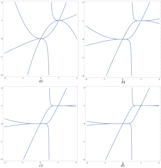
Figure 1 includes computer-generated sketches of the real loci of 𝒞⁡(n)\mathcal{C}(n) for some even values of nn; the graphs give compelling evidence for Conjectures 4.5 and 3.1.

Figure 1. Real loci of a) P2=0P_{2}=0, b) P4=0P_{4}=0, c) P6=0P_{6}=0, and d) P8=0P_{8}=0.

The affirmation of Conjecture 4.6 is a consequence by the monotonicity property of Conjecture 4.5, together with the conjectural characterization 4.3 of the real singular points of 𝒞⁡(n)¯\overline{\mathcal{C}(n)}. In particular, Conjecture 4.6 holds when n=5n=5.

It remains to verify Conjecture 4.5 when n=5n=5. To this end, first note that implicitly differentiating the equation Pn​(x,λ⁡(x))=0P_{n}(x,\lambda(x))=0 with respect to xx shows that

d​λd​x=0⇔d​Pnd​x=0\frac{d\lambda}{dx}=0\iff\frac{dP_{n}}{dx}=0

away from the singular points of 𝒞⁡(n)\mathcal{C}(n). On the other hand, for small values of nn (including n=5n=5), the equations Pn=d​Pnd​x=0P_{n}=\frac{dP_{n}}{dx}=0 have no common affine solutions (x,y)(x,y) in ℝ2∖{(0,0),(1,1)}\mathbb{R}^{2}\setminus\{(0,0),(1,1)\}. In light of the Puiseux parametrizations of the real branches near (0,0)(0,0) and the symmetries (4.2), the desired xx-monotonicity properties of the solution curves λ=λ⁡(x)\lambda=\lambda(x) follow immediately. It suffices now to check that P5​(x,λ)=0P_{5}(x,\lambda)=0 has exactly three solutions λ\lambda for each fixed value of xx in ℝ∖{0,1,12}\mathbb{R}\setminus\{0,1,\frac{1}{2}\}, i.e. that 𝒞​(5)​(ℝ)\mathcal{C}(5)(\mathbb{R}) is connected over each of the critical intervals (−∞,0)(-\infty,0), (0,1)(0,1), and (1,∞)(1,\infty) in xx. But this, in turn, is an immediate consequence of the Implicit Function theorem.

Finally, it remains to verify the inequalities of the real solution curves λ=λ⁡(x)\lambda=\lambda(x) described in the topological profile of 𝒞⁡(3)\mathcal{C}(3) above relative to xx. These hold locally near the singular points (0,0)(0,0) and (1,1)(1,1) of 𝒞⁡(5)\mathcal{C}(5) in the affine plane, so it suffices simply to show that the intersection of the line y=xy=x with 𝒞​(5)​(ℝ)\mathcal{C}(5)(\mathbb{R}) is precisely supported along {(0,0),(1,1)}\{(0,0),(1,1)\}. And indeed, we have

P5​(x,x)=−10532​x5+52532​x6−52516​x7+52516​x8−52532​x9+10532​x10=−10532​x5​(x−1)5.P_{5}(x,x)=-\frac{105}{32}x^{5}+\frac{525}{32}x^{6}-\frac{525}{16}x^{7}+\frac{525}{16}x^{8}-\frac{525}{32}x^{9}+\frac{105}{32}x^{10}=-\frac{105}{32}x^{5}(x-1)^{5}.

∎

Figure 2 includes sketches of the the real loci of 𝒞⁡(n)\mathcal{C}(n) for small odd values of nn; just as in Figure 1, the validity of Conjectures 4.5 and 3.1 in these cases is graphically apparent.
Refer to caption
Figure 2. Real loci of a) P3=0P_{3}=0, b) P5=0P_{5}=0, c) P7=0P_{7}=0, and d) P9=0P_{9}=0.

5. From incomplete series on an elliptic curve to complete series on a hyperelliptic curve

Conjectures 4.5 and 3.1, assuming they hold, may be leveraged to construct complete real linear series on real hyperelliptic curves of genus g≥1g\geq 1 with many real inflection points.

Theorem 5.1.

Assume that Conjecture 3.1 holds. There exists a maximally-real hyperelliptic curve XX with affine equation y2=fy^{2}=f admits a complete real linear series |ℒℝ|=|ℒℝ​(k​D)||\mathcal{L}_{\mathbb{R}}|=|\mathcal{L}_{\mathbb{R}}(kD)| with the distinguished basis ℱg\mathcal{F}_{g} as in (1) whose total real inflectionary degree is

ωℝ​(k,g)=2​g​(g+1)+2​(k−g)​(g−1)+2​g​(1+gmod2)​(k−g).\omega_{\mathbb{R}}(k,g)=2g(g+1)+2(k-g)(g-1)+2g(1+g\hskip-7.0pt\mod 2)(k-g).

Here f=f⁡(x)f=f(x) is a polynomial of degree 2​g−12g-1 ramified over ∞∈ℙ1\infty\in\mathbb{P}^{1}, and DD is the divisor represented by the pullback of ∞\infty to XX.

Proof.

Follows immediately from Theorems 5.8 and 6.1 of [1]. ∎

References

  • [1] I. Biswas, E. Cotterill, and C. Garay López, Real inflection points of real hyperelliptic curves, arXiv:1708.08400.
  • [2] E. Brieskorn and H. Knörrer, “Plane algebraic curves”, Springer, 1986.
  • [3] C. Garay, Tropical intersection theory, and real inflection points of real algebraic curves, Univ. Paris VI doctoral thesis, 2015.
  • [4] P. Griffiths and J. Harris, On Cayley’s explicit solution to Poncelet’s porism, Enseign. Math. 24 (1978), 31–40.
  • [5] J. Silverman, “The arithmetic of elliptic curves”, Springer, 1985.