Generalized trace distance approach to quantum non-Markovianity and detection of initial correlations

To introduce the concept of information, which proves to be fundamental in all this work, we consider two parties, Alice and Bob [5, 8]: Alice prepares the system in two possible quantum states $\rho^{1}$ and $\rho^{2}$, with respective probabilities $p_{1}$ and $p_{2}$, with $p_{1},p_{2}\geq 0$ and $p_{1}+p_{2}=1$, and then sends it to Bob. Bob has the task to figure out, by means of a single measurement, whether the system has been prepared in the state $\rho^{1}$ or $\rho^{2}$ (see Figure 1). The success probability in the discrimination procedure, if the measurement is carried out by means of two positive operators $\{P_{1},P_{2}\}$ such that $P_{1},P_{2}\geq 0$ and $P_{1}+P_{2}=I$, is

$$p_{\textrm{success}}(t)=p_{1}\Tr[P_{1}\rho^{1}(t)]+p_{2}\Tr[P_{2}\rho^{2}(t)].$$

Expressing $P_{1}$ in function of $P_{2}$ and vice versa one gets

$$p_{\textrm{success}}(t)=p_{2}+\Tr[P_{1}\Delta(t)]=p_{1}-\Tr[P_{2}\Delta(t)],$$

(1)

where we have defined the Helstrom matrix

$$\Delta(t)=p_{1}\rho^{1}(t)-p_{2}\rho^{2}(t).$$

(2)

Hence, one can recast (1) as

	$\displaystyle p_{\textrm{success}}(t)=$	$\displaystyle\frac{1}{2}{[}p_{2}+\Tr[P_{1}\Delta(t)]+p_{1}-\Tr[P_{2}\Delta(t)]{]}$
	$\displaystyle=$	$\displaystyle\frac{1}{2}{[}1+\Tr[(P_{1}-P_{2})\Delta(t)]{]},$

which is maximal if $P_{1}$ and $P_{2}$ are the projectors on the subspaces spanned by the positive and negative eigenvectors of $\Delta(t)$ respectively, and, in that case, is equal to

$$p^{\textrm{max}}_{\textrm{success}}(t)=\frac{1}{2}{[}1+||\Delta(t)||{]}.$$

The trace norm of the Helstrom matrix is connected to the information which can be obtained measuring the evolved states, because it provides the bias in favor of their distinguishability. Note that considering initial equal preparation frequencies $p_{1}=p_{2}=1/2$, the trace norm of (2) reduces to the trace distance between the states [27]

$$D(\rho^{1}(t),\rho^{2}(t))=\frac{1}{2}\Tr|\rho^{1}(t)-\rho^{2}(t)|,$$

which is maximal and equal to one for orthogonal states, i.e. with orthogonal support, while zero for equal density matrices.

The evolution in time of the distinguishability between the initial states prepared by Alice is related to the character of the dynamics. If one considers a closed and isolated quantum system, such as the total system $S+E$, whose evolution is described by time-dependent unitary operators $\{U_{t}\}_{t}$, acting on density operators as $\rho_{SE}(t)=U_{t}\rho_{SE}U_{t}^{\dagger}$, $||p_{1}\rho_{SE}^{1}(t)-p_{2}\rho_{SE}^{2}(t)||=||p_{1}\rho_{SE}^{1}-p_{2}\rho_{SE}^{2}||$. In fact unitary transformations do not change the spectrum of operators. We define this conserved quantity as total information in the composite system $S+E$

$$\mathcal{I}_{\textrm{tot}}(t)=||p_{1}\rho_{SE}^{1}(t)-p_{2}\rho_{SE}^{2}(t)||.$$

However, the open quantum system $S$ undergoes non-unitary dynamics, derived from the underlying global coherent evolution by tracing over the environmental degrees of freedom

$$\rho_{S}=\Tr_{E}\rho_{SE}\textrm{ }\mapsto\textrm{ }\rho_{S}(t)=\Tr_{E}[U_{t}\rho_{SE}U_{t}^{\dagger}].$$

(3)

Hence, the distinguishability between reduced states can vary in time. We define the internal information as the information accessible by Bob, if he is allowed to perform measurements on the open quantum system $S$ only

$$\mathcal{I}_{\textrm{int}}(t)=||p_{1}\rho_{S}^{1}(t)-p_{2}\rho_{S}^{2}(t)||.$$

Consequently, we define the external information as

	$\displaystyle\mathcal{I}_{\textrm{ext}}(t)=$	$\displaystyle\textrm{ }\mathcal{I}_{\textrm{tot}}(t)-\mathcal{I}_{\textrm{int}}(t)$
	$\displaystyle=$	$\displaystyle\textrm{ }||p_{1}\rho_{SE}^{1}(t)-p_{2}\rho_{SE}^{2}(t)||-||p_{1}\rho_{S}^{1}(t)-p_{2}\rho_{S}^{2}(t)||.$

Hence, the conservation of the total information, in terms of internal and external information at different times $t,s\geq 0$, can be written as a balance equation

$$\mathcal{I}_{\textrm{int}}(t)+\mathcal{I}_{\textrm{ext}}(t)=\mathcal{I}_{\textrm{int}}(s)+\mathcal{I}_{\textrm{ext}}(s).$$

(4)

In this section we present an inequality for the external information, as captured by the trace norm of Helstrom matrices, which generalizes the inequality derived for the trace distance case [4]. This is the main finding of this article. The inequality represents an important result because it allows to extend the interpretation of non-Markovianity in terms of the flow of information between the open system and its environment to case when the distinguishability is measured in terms of the trace norm of the Helstrom matrix.

The external information at a given time $t$ is nonzero if correlations in the global states $\rho_{SE}^{1,2}(t)$ are present or the environmental marginals are different, as expressed by the following inequality

	$\displaystyle\mathcal{I}_{\textrm{ext}}(t)\leq$	$\displaystyle 2p_{1}D(\rho_{SE}^{1}(t),\rho_{S}^{1}(t)\otimes\rho_{E}^{1}(t))$		(5)
	$\displaystyle+$	$\displaystyle 2p_{2}D(\rho_{SE}^{2}(t),\rho_{S}^{2}(t)\otimes\rho_{E}^{2}(t))$
	$\displaystyle+$	$\displaystyle 2\min\{p_{1},p_{2}\}D(\rho_{E}^{1}(t),\rho_{E}^{2}(t)).$

The trace distance case [4] can be trivially retrieved by setting $p_{1}=p_{2}=1/2$. The proof is given in the appendix.

The possibility to introduce reduced dynamical maps, i.e. maps acting on the open quantum system degrees of freedom only describing its dynamics, treating effectively the presence of the environment, rests on the condition of initially factorized states $\rho_{SE}=\rho_{S}\otimes\rho_{E}$, with a fixed marginal state of the environment. In fact, in such case the quantum process ${\Phi}$ is given by a collection of trace-preserving time-dependent maps $\{\Phi_{t}\}_{t}$, which are completely positive [30, 31], defined via

$$\Phi_{t}\rho_{S}=\Tr_{E}[U_{t}\rho_{S}\otimes\rho_{E}U_{t}^{\dagger}].$$

Definition. A quantum process ${\Phi}$ is Markovian if $||p_{1}\Phi_{t}\rho_{S}^{1}-p_{2}\Phi_{t}\rho_{S}^{2}||$ is a monotonic decreasing function of time, for any $p_{1},p_{2}\geq 0$ with $p_{1}+p_{2}=1$ and $\rho_{S}^{1},\rho_{S}^{2}\in\mathcal{S}(\mathcal{H}_{S})$ [8].

An interpretation via information flow between the system and the environment has been devised for the original definition of quantum non-Markovianity [5, 22], and as shown here via Eq. (5) it can be generalized for the new definition in a straightforward way.

In case of initially factorized states $\rho_{SE}^{1,2}=\rho_{S}^{1,2}\otimes\rho_{E}$, which is a premise to introduce reduced dynamical maps and, hence, talk about a quantum process, we have that total and internal information at initial time do coincide. In fact, we have

	$\displaystyle\mathcal{I}_{\textrm{tot}}(0)=$	$\displaystyle\textrm{ }||p_{1}\rho_{S}^{1}\otimes\rho_{E}-p_{2}\rho_{S}^{2}\otimes\rho_{E}||$
	$\displaystyle=$	$\displaystyle\textrm{ }||p_{1}\rho_{S}^{1}-p_{2}\rho_{S}^{2}||\textrm{ }||\rho_{E}||=\mathcal{I}_{\textrm{int}}(0)$

and, consequently, $\mathcal{I}_{\textrm{ext}}(0)=0$. Thus, recasting the equation for the conservation of the total information (4), choosing $s=0$ the initial time, we have

$$\mathcal{I}_{\textrm{int}}(0)-\mathcal{I}_{\textrm{int}}(t)=\mathcal{I}_{\textrm{ext}}(t)\geq 0,$$

which express the fact that the internal information is always bounded from above by its initial value. This is of course in agreement with the contraction property of the trace norm under (completely) positive and trace preserving reduced dynamical maps [32].

Let us now consider the equation for the conservation of the total information (4): a backflow of information, captured by an increase of the internal information between $s>0$ and the later time $t$, can be present only if the external information is non zero at the former time. In fact

	$\displaystyle\mathcal{I}_{\textrm{int}}(t)-\mathcal{I}_{\textrm{int}}(s)=$	$\displaystyle\textrm{ }\mathcal{I}_{\textrm{ext}}(s)-\mathcal{I}_{\textrm{ext}}(t)$		(6)
	$\displaystyle\leq$	$\displaystyle\textrm{ }\mathcal{I}_{\textrm{ext}}(s),$

because $\mathcal{I}_{\textrm{ext}}(t)$ is a positive quantity. The interpretation of the external information, for this generalized definition with the trace norm of Helstrom matrices, as presence of correlations in the states $\rho_{SE}^{1,2}(s)$ or as different environmental states is expressed by inequality (5).

In case the assumption of initially factorized states is violated, there is in general no possibility to introduce reduced dynamical maps and hence speak of a quantum process, let alone of Markovianity and non-Markovianity. However, the interpretation via flow of information is still valid and can be used to witness locally the presence of initial correlations in the global system-environment states [19]. Here we show a generalization of the bound presented in [4, 19], considering the trace norm of Helstrom matrices in place of the trace distances of states. Setting $s=0$ on right-hand side of (6), we get

	$\displaystyle\mathcal{I}_{\textrm{int}}(t)-\mathcal{I}_{\textrm{int}}(0)=$	$\displaystyle\textrm{ }\mathcal{I}_{\textrm{ext}}(0)-\mathcal{I}_{\textrm{ext}}(t)$		(7)
	$\displaystyle\leq$	$\displaystyle\textrm{ }\mathcal{I}_{\textrm{ext}}(0)$

and, by means of (5), we obtain the generalized bound for the increase of internal information with respect to its initial value

	$\displaystyle\mathcal{I}_{\textrm{int}}(t)-\mathcal{I}_{\textrm{int}}(0)\leq$	$\displaystyle\textrm{ }2p_{1}D(\rho_{SE}^{1},\rho_{S}^{1}\otimes\rho_{E}^{1})$		(8)
	$\displaystyle+$	$\displaystyle\textrm{ }2p_{2}D(\rho_{SE}^{2},\rho_{S}^{2}\otimes\rho_{E}^{2})$
	$\displaystyle+$	$\displaystyle\textrm{ }2\min\{p_{1},p_{2}\}D(\rho_{E}^{1},\rho_{E}^{2}),$

which links a possible increase of internal information above the intial value to different environmental initial states or correlations in the total initial states.

To show that the generalized bound (3.2) can indeed lead to a better sensitivity in detecting initial correlations we provide an explicit example.

We consider a two-level system subjected to a pure dephasing dynamics, generated by the interaction with a bosonic mode, through the full Hamiltonian

$$H=H_{S}\otimes I_{E}+I_{S}\otimes H_{E}+S\otimes X,$$

(9)

where $S\otimes X$ is the interaction term between the system and the environment satisfying

$$[H_{S},S]=0.$$

This condition ensures that $H_{S}$ is a conserved quantity, because $[H_{S},H]=0$ and enables to carry out analytical calculations. In particular, we take in (9)

	$\displaystyle H_{S}=$	$\displaystyle\textrm{ }\epsilon\sigma_{S}^{3},$
	$\displaystyle H_{E}=$	$\displaystyle\textrm{ }\omega b^{\dagger}b,$
	$\displaystyle S\otimes X=$	$\displaystyle\textrm{ }g\sigma_{S}^{3}\otimes(b+b^{\dagger}),$

where $b$ and $b^{\dagger}$ are lowering and raising operators of the bosonic mode, $g$ is the coupling constant, while $\epsilon$ and $\omega$ are the energy spacing between the eigenstates of the system and the environment respectively, in the units where $\hbar=1$. We consider, as initial condition for our dynamical evolution, states depending on the parameter $\lambda\in[0,1]$ of the form [33, 34]

$$\left|\Psi_{\lambda}(0)\right\rangle_{SE}=\alpha\left|1\right\rangle\otimes\left|0\right\rangle_{E}+\beta\left|0\right\rangle\otimes\left|\Omega_{\lambda}\right\rangle_{E},$$

(10)

where $\left|k\right\rangle$, with $k=1,0$, are respectively the excited and ground states of the two level system, while $\left|0\right\rangle_{E}$ and $\left|\Omega_{\lambda}\right\rangle_{E}$ are states of the bosonic mode. We require $|\alpha|^{2}+|\beta|^{2}=1$ to ensure normalization of $\left|\Psi_{\lambda}(0)\right\rangle_{SE}$. The field state is given by the coherent superposition of the vacuum state of the bosonic mode $\left|0\right\rangle_{E}$ and a certain coherent state $\left|y\right\rangle_{E}$, that is

$$\left|\Omega_{\lambda}\right\rangle_{E}=\frac{1}{C_{\lambda}}[(1-\lambda)\left|0\right\rangle_{E}+\lambda\left|y\right\rangle_{E}],$$

(11)

with $b\left|y\right\rangle_{E}=y\left|y\right\rangle_{E}$, while the normalization factor reads

$$C_{\lambda}=\sqrt{(1-\lambda)^{2}+\lambda^{2}+2\lambda(1-\lambda)\textrm{ Re}({}_{E}\langle 0|y\rangle_{E})}.$$

This state reduces to the vacuum state for $\lambda=0$, so that the initial composite state (10) is factorized. Otherwise, aside from $\alpha=0$ or $\beta=0$, we have an initial state $\left|\Psi_{\lambda}(0)\right\rangle_{SE}$ that is not factorized, but is actually entangled.

The dynamical evolution of the reduced state of the system (3) can be studied through the evolution of its matrix elements $\left\langle i\right|\rho_{S}(t)\left|j\right\rangle$, where $\left|i\right\rangle,\left|j\right\rangle$ are the eigenvectors of the system free Hamiltonian $H_{S}=\epsilon\sigma_{S}^{3}$. The expression has been derived in [33, 34] and, upon choosing the coherent state $\left|y\right\rangle_{E}$ in $\left|\Omega_{\lambda}\right\rangle_{E}$ (11) to be $\left|y=1\right\rangle_{E}$, reads

$$\rho^{\lambda}_{S}(t)=\begin{pmatrix}|\alpha|^{2}&\alpha\beta^{*}B_{\lambda}(t)\\ \alpha^{*}\beta B^{*}_{\lambda}(t)&|\beta|^{2}\end{pmatrix},$$

where $\rho_{S}^{\lambda}(t)=\Tr_{E}[\left|\Psi_{\lambda}(t)\right\rangle_{SE}\left\langle\Psi_{\lambda}(t)\right|]$, with

$$B_{\lambda}(t)=\frac{1}{C_{\lambda}}e^{-2i\epsilon t}e^{-R(t)},$$

and

	$\displaystyle R(t)=$	$\displaystyle\textrm{ }4\left(\frac{g}{\omega}\right)^{2}[1-\cos(\omega t)],$		(12)
	$\displaystyle\Lambda(t)=$	$\displaystyle\textrm{ }\frac{g}{\omega}\sin(\omega t),$
	$\displaystyle S(t)=$	$\displaystyle\textrm{ }2\frac{g}{\omega}[1-\cos(\omega t)]-\frac{1}{2}.$

Therefore, to study the efficiency of this local scheme for the detection of initial correlations, we consider the reduced system states $\rho_{S}^{0}$, which is initially factorized, and $\rho_{S}^{\lambda}$, with the parameter $\lambda$ entailing the quantity of correlations in the initial global state. Their Helstrom matrices

	$\displaystyle\Delta(t)=$	$\displaystyle\textrm{ }p_{1}\rho_{S}^{\lambda}(t)-p_{2}\rho_{S}^{0}(t)$		(13)
	$\displaystyle=$	$\displaystyle\textrm{ }\begin{pmatrix}(p_{1}-p_{2})|\alpha|^{2}&\alpha\beta^{*}e^{-2i\epsilon t}e^{-R(t)}\\ h.c.&(p_{1}-p_{2})|\beta|^{2}\end{pmatrix},$

are functions of $p_{1}$, $\alpha$ and $\beta$, upon choosing the physical parameters of the model as $\epsilon=1$, $\omega=1$ and $g=0.1$, in agreement with the literature [33, 34].

We carry out numerical simulations to find the probability of detecting initial correlations with the novel approach, comparing the results with the performance of the old approach used in [34]. It is important to note that, in such article, the authors confront the efficiency of different distance measures, namely the trace distance, the Bures metric, the Hellinger distance and the Jensen-Shannon divergence [35], with the first one being the most effective: here thus we compare the trace distance with the trace norm of the Helstrom matrix.

To this end, for each considered value of $p_{1}\in[0,1]$ and $\lambda\in[0,1]$, we determine the probability of an increase in time of the internal information with respect to its initial value: we randomly draw $500$ pairs $\{\alpha,\beta\}$ in their range of variability and determine the frequency of detection of initial correlations. The maximum time considered in this computation is $t=2\pi$, corresponding to the period of the oscillating quantities (12) in (13), and the evolved internal information is computed with a time step $\textrm{d}t=0.15$. The result is depicted in Figure 2.

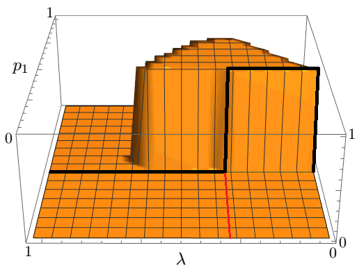
The graph shows a threshold value in detection of initial correlations, when using the trace distance [34]: in fact, for $\lambda\gtrsim 0.4$ and $p_{1}=1/2$ there is no increase of internal information with respect to its initial value. Nonetheless, if one considers the novel approach and chooses $p_{1}>1/2$ - giving, hence, more weight to the correlated state in the Helstrom matrix (13) - one can better detect initial correlations, witnessing them for $\lambda>0.4$.

To stress this better detection capability, we plot, for different values of $\lambda$ around the threshold value $0.4$, the trace distance and the trace norm of (13) with $p_{1}=0.6$ as functions of time and the free parameters $\{\alpha,\beta\}$. In this case $\alpha,\beta\in\mathbb{R}$, with $\beta=\sqrt{1-|\alpha|^{2}}$. As we can see from Figure 3, no initial increase is observed after the threshold value $\lambda\sim 0.4$ using the trace distance, while the novel approach with $p_{1}=0.6$ stops witnessing correlations around $\lambda\sim 0.7$.

The idea of information has been interestingly used also to devise a method to detect quantum correlations [36, 37, 38] in a composite system using only local operations [20, 39]. This method has been experimentally realized for both trapped ions [40] and photonic systems [41, 42].

The basic idea behind such method is to consider the evolution of the internal information between the composite state of interest $\rho_{SE}$ and the state $\rho^{\prime}_{SE}=(\Phi_{d}\otimes I_{E})\rho_{SE}$, where $\Phi_{d}$ is the local map acting as

$$\Phi_{d}X=\sum_{j=1}^{n}\Pi_{S}^{j}X\Pi_{S}^{j},$$

with $\{\Pi_{S}^{j}\}_{j=1,...,n}$ the complete set of rank-one orthogonal projectors on the eigenstates of $\rho_{S}$, namely $\rho_{S}=\sum_{j=1}^{n}q_{j}\Pi_{S}^{j}$, where $n=\textrm{dim}\mathcal{H}_{S}$. Thus the corresponding composite state change is given by

$$\rho^{\prime}_{SE}=\sum_{j=1}^{n}q_{j}\Pi_{S}^{j}\otimes\rho_{E}^{j},$$

(14)

with

$$\rho_{E}^{j}=\frac{\Tr_{S}[(\Pi_{S}^{j}\otimes I_{E})\rho_{SE}(\Pi_{S}^{j}\otimes I_{E})]}{\Tr_{SE}[(\Pi_{S}^{j}\otimes I_{E})\rho_{SE}]}$$

(15)

and

$$q_{j}=\Tr_{SE}[(\Pi_{S}^{j}\otimes I_{E})\rho_{SE}].$$

(16)

Note that $\Phi_{d}$ can be built through local operations, i.e. only performing measurements on the reduced state.

Although the open system states are identical at the initial time, their global counterparts $\rho_{SE}$ and $\rho^{\prime}_{SE}$ are identical only if $\rho_{SE}$ is originally a zero quantum discord state of the form (14). This leads to possible differences in the time evolution of the reduced open system states, so that

$$D(\rho_{S}(t),\rho^{\prime}_{S}(t))=\frac{1}{2}||\Tr_{E}[U_{t}(\rho_{SE}-\rho^{\prime}_{SE})U_{t}^{\dagger}]||>0$$

(17)

has been considered as a witness for quantum correlations in $\rho_{SE}$.

Here, we demonstrate that the local detection method can be generalized by using the norm of Helstrom matrices as quantifiers for state discrimination. Thus, we consider $\mathcal{I}_{\textrm{int}}(t)=||p_{1}\rho_{S}(t)-p_{2}\rho^{\prime}_{S}(t)||$, and we propose as a novel condition for the detection of initial quantum correlations

$$\mathcal{I}_{\textrm{int}}(t)-\mathcal{I}_{\textrm{int}}(0)>0,$$

(18)

where, in particular, we have $\mathcal{I}_{\textrm{int}}(0)=|p_{1}-p_{2}|$.

The interpretation via flow of information between the system and the environment is captured by the following upper bound for the increase of internal information proven in appendix

$$\mathcal{I}_{\textrm{int}}(t)-\mathcal{I}_{\textrm{int}}(0)\leq 2\min\{p_{1},p_{2}\}\textrm{ }D(\rho_{SE},\rho^{\prime}_{SE}),$$

(19)

so that the maximum increase of internal information is captured via the trace distance between $\rho_{SE}$ and the classically correlated $\rho_{SE}^{\prime}$.

It is important to notice that this novel approach leads to no improvements in the detection of quantum correlations. In fact, on the one hand, both witnesses (17) and (18) are able to detect initial correlations if and only if

$$\rho_{S}(t)\neq\rho_{S}^{\prime}(t)$$

for some $t>0$. Thus, the use of the trace norm of the Helstrom matrix does not improve the capability of detecting quantum correlations. On the other hand, the bound for the increase of internal information, given by inequality (19), is maximal for $p_{1}=p_{2}=1/2$, which indicates that the new witness is not more sensitive than the witness based on the trace distance, which therefore turns out to be the optimal one.

We now focus on a specific example with low dimensional system and environment. This enables the evaluation of the r.h.s. of the bound (19), which requires the computation of the trace distance of system and environment states. We thus consider the model originally proposed in [19] consisting of a couple of two-level systems undergoing a CNOT quantum gate [27]. Thus we will not study the continuum time evolution of the internal information, but we will just compute and compare the initial value $\mathcal{I}_{\textrm{int}}(0)$, with the one after the state transformation has occurred, that we still indicate with $\mathcal{I}_{\textrm{int}}(t)$. The action of the CNOT can be defined by

	$\displaystyle U_{C}\left|11\right\rangle=$	$\displaystyle\left|11\right\rangle,\quad\quad U_{C}\left|10\right\rangle=\left|10\right\rangle,$
	$\displaystyle U_{C}\left|01\right\rangle=$	$\displaystyle\left|00\right\rangle,\quad\quad U_{C}\left|00\right\rangle=\left|01\right\rangle,$

where $\left|ij\right\rangle\left\langle kl\right|=\left|i\right\rangle\left\langle k\right|\otimes\left|j\right\rangle\left\langle l\right|$ for any $i,j,k,l\in\{0,1\}$ and $\sigma^{3}\left|j\right\rangle=(-1)^{j+1}\left|j\right\rangle$. We consider the families of initial states [43]

	$\displaystyle\rho_{SE}=$	$\displaystyle\textrm{ }(\alpha\left|11\right\rangle+\beta\left|00\right\rangle)(\alpha^{*}\left\langle 11\right|+\beta^{*}\left\langle 00\right|)$		(20a)
	$\displaystyle\rho^{\prime}_{SE}=$	$\displaystyle\textrm{ }|\alpha|^{2}\left|11\right\rangle\left\langle 11\right|+|\beta|^{2}\left|00\right\rangle\left\langle 00\right|,$		(20b)

with $|\alpha|^{2}+|\beta|^{2}+=1$, which are respectively pure entangled states and their classically correlated version, i.e. $\rho^{\prime}_{SE}=\Phi_{d}\rho_{SE}$, as explained in Sec. III.3 (see Appendix).

We know that $\mathcal{I}_{\textrm{int}}(0)=|p_{1}-p_{2}|$. The calculation of the evolved internal information is quite lengthy and worked out in the appendix with the result

		$\displaystyle\mathcal{I}_{\textrm{int}}(t)$		(21)
	$\displaystyle\textrm{ }$	$\displaystyle=\begin{cases}|p_{1}-p_{2}|&\text{if }p_{1}<1/3\\ \sqrt{(p_{1}-p_{2})^{2}(|\alpha|^{2}-|\beta|^{2})^{2}+4p_{1}^{2}|\alpha\beta|^{2}}&\text{if }p_{1}\geq 1/3.\end{cases}$

The bound (19), also computed in the appendix, reads

$$2\min\{p_{1},p_{2}\}D(\rho_{SE},\rho^{\prime}_{SE})=2\min\{p_{1},p_{2}\}\textrm{ }|\alpha\beta|.$$

(22)

We represent the increase of internal information and its bound in Figure 4. The plot is in accordance with the theoretical predictions, presented in the previous section: there are no initial quantum correlations that can be detected via the method which adopts the trace norm of Helstrom matrices, which cannot be detected using the trace distance. Moreover, the maximum increase of internal information is obtained, for any choice of the parameters $\alpha,\beta$ characterizing the state (20a), when $p_{1}=p_{2}=1/2$. In particular, in this example, there is no detection of initial quantum correlations when $p_{1}<1/3$, as indicated by the red line.

Using the property $||A\otimes B||=||A||\textrm{ }||B||$ and because $||\rho||=1$ for any statistical operator, we have

	$\displaystyle\mathcal{I}_{\textrm{ext}}(t)=$	$\displaystyle\textrm{ }||p_{1}\rho_{SE}^{1}(t)-p_{2}\rho_{SE}^{2}(t)||$		(23)
		$\displaystyle\textrm{ }-||(p_{1}\rho_{S}^{1}(t)-p_{2}\rho_{S}^{2}(t))\otimes\rho_{E}^{1}(t)||,$

but also

	$\displaystyle\mathcal{I}_{\textrm{ext}}(t)=$	$\displaystyle\textrm{ }||p_{1}\rho_{SE}^{1}(t)-p_{2}\rho_{SE}^{2}(t)||$		(24)
		$\displaystyle\textrm{ }-||(p_{1}\rho_{S}^{1}(t)-p_{2}\rho_{S}^{2}(t))\otimes\rho_{E}^{2}(t)||.$

Exploiting positivity of $\mathcal{I}_{\textrm{ext}}(t)$ from (23), using the triangular inequality twice, we obtain

		$\displaystyle\mathcal{I}_{\textrm{ext}}(t)$
		$\displaystyle\textrm{ }\leq||p_{1}\rho_{SE}^{1}(t)-p_{2}\rho_{SE}^{2}(t)-(p_{1}\rho_{S}^{1}(t)-p_{2}\rho_{S}^{2}(t))\otimes\rho_{E}^{1}(t)||$
		$\displaystyle\textrm{ }=||p_{1}[\rho_{SE}^{1}(t)-\rho_{S}^{1}(t)\otimes\rho_{E}^{1}(t)]-p_{2}[\rho_{SE}^{2}(t)-\rho_{S}^{2}(t)\otimes\rho_{E}^{1}(t)]||$
		$\displaystyle\textrm{ }\leq 2p_{1}D(\rho_{SE}^{1}(t),\rho_{S}^{1}(t)\otimes\rho_{E}^{1}(t))+2p_{2}D(\rho_{SE}^{2}(t),\rho_{S}^{2}(t)\otimes\rho_{E}^{1}(t)).$

Using the triangular inequality for the trace distance and the property

$$D(\rho_{S}^{2}(t)\otimes\rho_{E}^{2}(t),\rho_{S}^{2}(t)\otimes\rho_{E}^{1}(t))=D(\rho_{E}^{2}(t),\rho_{E}^{1}(t)),$$

we, hence, obtain

	$\displaystyle\mathcal{I}_{\textrm{ext}}(t)\leq$	$\displaystyle\textrm{ }2p_{1}D(\rho_{SE}^{1}(t),\rho_{S}^{1}(t)\otimes\rho_{E}^{1}(t))$
	$\displaystyle+$	$\displaystyle\textrm{ }2p_{2}D(\rho_{SE}^{2}(t),\rho_{S}^{2}(t)\otimes\rho_{E}^{2}(t))$
	$\displaystyle+$	$\displaystyle\textrm{ }2p_{2}D(\rho_{E}^{1}(t),\rho_{E}^{2}(t)).$

Analogously, from (24), we obtain

	$\displaystyle\mathcal{I}_{\textrm{ext}}(t)\leq$	$\displaystyle\textrm{ }2p_{1}D(\rho_{SE}^{1}(t),\rho_{S}^{1}(t)\otimes\rho_{E}^{1}(t))$
	$\displaystyle+$	$\displaystyle\textrm{ }2p_{2}D(\rho_{SE}^{2}(t),\rho_{S}^{2}(t)\otimes\rho_{E}^{2}(t))$
	$\displaystyle+$	$\displaystyle\textrm{ }2p_{1}D(\rho_{E}^{1}(t),\rho_{E}^{2}(t)),$

and therefore the claimed result (5).

We consider inequality (7), where in this case

$$\mathcal{I}_{\textrm{ext}}(0)=||p_{1}\rho_{SE}-p_{2}\rho^{\prime}_{SE}||-|p_{1}-p_{2}|,$$

because $\rho_{S}=\rho_{S}^{\prime}$ and $\mathcal{I}_{\textrm{int}}(0)$ reduces to $|p_{1}-p_{2}|$. In particular, because $|x|=|x|\textrm{ }||\rho||$ for any density operator $\rho$ and $x\in\mathbb{C}$, we have

$$\mathcal{I}_{\textrm{ext}}(0)=||p_{1}\rho_{SE}-p_{2}\rho^{\prime}_{SE}||-||(p_{1}-p_{2})\rho_{SE}||,$$

but also

$$\mathcal{I}_{\textrm{ext}}(0)=||p_{1}\rho_{SE}-p_{2}\rho^{\prime}_{SE}||-||(p_{1}-p_{2})\rho^{\prime}_{SE}||.$$

In both cases, because $\mathcal{I}_{\textrm{tot}}(0)\geq\mathcal{I}_{\textrm{int}}(0)$, we can use the triangular inequality for the trace norm in the form

$$\big|\textrm{ }||A||-||B||\textrm{ }\big|\leq||A-B||,$$

which leads, via (7), to

$$\mathcal{I}_{\textrm{int}}(t)-\mathcal{I}_{\textrm{int}}(0)\leq||p_{2}(\rho_{SE}-\rho^{\prime}_{SE})||$$

and

$$\mathcal{I}_{\textrm{int}}(t)-\mathcal{I}_{\textrm{int}}(0)\leq||p_{1}(\rho_{SE}-\rho^{\prime}_{SE})||$$

Hence, by definition of trace distance, we obtain the general bound (19).

Here we show the calculations needed to derive the results (21) and (22).

To this end, we first check the relation $\rho^{\prime}_{SE}=(\Phi_{d}\otimes I_{E})\rho_{SE}$ for the global states defined in (20a) and (20b). Because the marginal state is $\rho_{S}=\Tr_{E}\rho_{SE}=|\alpha|^{2}\left|0\right\rangle\left\langle 0\right|+|\beta|^{2}\left|1\right\rangle\left\langle 1\right|$, we have

$$\Phi_{d}X=\sum_{j=1,0}\Pi_{S}^{j}X\Pi_{S}^{j},$$

with $\Pi_{S}^{1}=\left|1\right\rangle\left\langle 1\right|$ and $\Pi_{S}^{0}=\left|0\right\rangle\left\langle 0\right|$. Computing $q_{j}$ as in (16), we have

$$q_{1}=|\alpha|^{2},\quad q_{0}=|\beta|^{2},$$

while $\rho_{E}^{j}$ as in (15) are

	$\displaystyle\rho_{E}^{1}=$	$\displaystyle\textrm{ }\frac{1}{|\alpha|^{2}}|\alpha|^{2}\left|1\right\rangle\left\langle 1\right|=\left|1\right\rangle\left\langle 1\right|,$
	$\displaystyle\rho_{E}^{0}=$	$\displaystyle\textrm{ }\frac{1}{|\beta|^{2}}|\beta|^{2}\left|0\right\rangle\left\langle 0\right|=\left|0\right\rangle\left\langle 0\right|.$

It is easy to see that $\rho^{\prime}_{SE}=(\Phi_{d}\otimes I_{E})\rho_{SE}$.

Secondly we compute the result of Eq. (21). The transformation of the states $\rho_{SE}$, as in (20a), and $\rho^{\prime}_{SE}$, as in (20b), under the CNOT is

	$\displaystyle U_{C}\rho_{SE}U_{C}^{\dagger}=$	$\displaystyle\textrm{ }(\alpha\left|11\right\rangle+\beta\left|01\right\rangle)\textrm{ }(\alpha^{*}\left\langle 11\right|+\beta^{*}\left\langle 01\right|),$
	$\displaystyle U_{C}\rho^{\prime}_{SE}U_{C}^{\dagger}=$	$\displaystyle\textrm{ }|\alpha|^{2}\left|11\right\rangle\left\langle 11\right|+|\beta|^{2}\left|01\right\rangle\left\langle 01\right|.$

Hence, the transformed marginals of the system are

	$\displaystyle\Tr_{E}[U_{C}\rho_{SE}U_{C}^{\dagger}]=$	$\displaystyle\textrm{ }|\alpha|^{2}\left|1\right\rangle\left\langle 1\right|+|\beta|^{2}\left|0\right\rangle\left\langle 0\right|$
	$\displaystyle+$	$\displaystyle\textrm{ }\alpha\beta^{*}\left|1\right\rangle\left\langle 0\right|+\alpha^{*}\beta\left|0\right\rangle\left\langle 1\right|,$
	$\displaystyle\Tr_{E}[U_{C}\rho^{\prime}_{SE}U_{C}^{\dagger}]=$	$\displaystyle\textrm{ }|\alpha|^{2}\left|1\right\rangle\left\langle 1\right|+|\beta|^{2}\left|0\right\rangle\left\langle 0\right|.$

Thus, we have that $\mathcal{I}_{\textrm{int}}(t)=||p_{1}\Tr_{E}[U_{C}\rho_{SE}U_{C}^{\dagger}]-p_{2}\Tr_{E}[U_{C}\rho^{\prime}_{SE}U_{C}^{\dagger}]||$ is equal to the trace norm of the Helstrom matrix

$$\Delta=\begin{pmatrix}(p_{1}-p_{2})|\alpha|^{2}&p_{1}\alpha\beta^{*}\\ p_{1}\alpha^{*}\beta&(p_{1}-p_{2})|\beta|^{2}\end{pmatrix}=\begin{pmatrix}\gamma&\theta\\ \theta^{*}&\delta\end{pmatrix},$$

(25)

having introduced

	$\displaystyle\gamma=$	$\displaystyle\textrm{ }(p_{1}-p_{2})|\alpha|^{2},$
	$\displaystyle\delta=$	$\displaystyle\textrm{ }(p_{1}-p_{2})|\beta|^{2},$
	$\displaystyle\theta=$	$\displaystyle\textrm{ }p_{1}\alpha\beta^{*}.$

The eigenvalues of (25) are

$$\eta_{\pm}=\frac{\gamma+\delta\pm\sqrt{(\gamma-\delta)^{2}+4|\theta|^{2}}}{2},$$

so that the trace norm of (25) is

		$\displaystyle||\Delta||$		(26)
		$\displaystyle=\begin{cases}|\gamma+\delta|&\quad\text{if }|\gamma+\delta|>\sqrt{(\gamma-\delta)^{2}+4|\theta|^{2}}\\ \sqrt{(\gamma-\delta)^{2}+4|\theta|^{2}}&\quad\text{if }|\gamma+\delta|\leq\sqrt{(\gamma-\delta)^{2}+4|\theta|^{2}}\end{cases}.$

To express (26) in terms of the original parameters $\alpha$, $\beta$ and $p_{1}$, we note that $\gamma+\delta=p_{1}-p_{2}$ and

$$(\gamma-\delta)^{2}+4|\theta|^{2}=(p_{1}-p_{2})^{2}(|\alpha|^{2}-|\beta|^{2})^{2}+4p_{1}^{2}|\alpha\beta|^{2},$$

so that the separating condition in (26) reads

$$(p_{1}-p_{2})^{2}-(p_{1}-p_{2})^{2}(|\alpha|^{2}-|\beta|^{2})^{2}+4p_{1}^{2}|\alpha\beta|^{2}\lessgtr 0.$$

(27)

Because $|\alpha|^{2}+|\beta|^{2}=1$, we can choose the parametrization $|\alpha|=\cos(z)$ and $|\beta|=\sin(z)$, with $z\in[0,\pi/2]$, so that (27) corresponds to

	$\displaystyle 0$	$\displaystyle\lessgtr\textrm{ }(p_{1}-p_{2})^{2}-(p_{1}-p_{2})^{2}\cos^{2}(2z)-p_{1}^{2}\sin^{2}(2z)$
		$\displaystyle=\textrm{ }\sin^{2}(2z)[(p_{1}-p_{2})^{2}-p_{1}^{2}].$

Thus, trivially, one obtains $(2p_{1}-1)^{2}-p_{1}^{2}\lessgtr 0$, which leads to the desired result (21).

References

- [1] H.-P. Breuer and F. Petruccione, The Theory of Open Quantum Systems, (Oxford University Press, Oxford, 2007)
- [2] V. Gorini, A. Kossakowski and E. C. G. Sudarshan, J. Math. Phys. 17, 821 (1976)
- [3] G. Lindblad, Comm. Math. Phys. 48, 119 (1976)
- [4] H.-P. Breuer, E.-M. Laine, J. Piilo and B. Vacchini, Rev. Mod. Phys. 88, 021002 (2016)
- [5] H.-P. Breuer, E.-M. Laine and J. Piilo, Phys. Rev. Lett. 103, 210401 (2009)
- [6] Á. Rivas, S. F. Huelga and M. B. Plenio, Phys. Rev. Lett. 105, 050403 (2010)
- [7] D. Chruściński, A. Kossakowski and A. Rivas, Phys. Rev. A 83, 52128 (2011)
- [8] S. Wißmann, B. Vacchini and H.-P. Breuer, Phys. Rev. A 92, 042108 (2015)
- [9] B.-H. Liu et al., Nature Phys. 7, 931 (2011)
- [10] B.-H. Liu et al., Sci. Rep. 3, 1781 (2013a)
- [11] M. Wittemer, G. Clos, H.-P. Breuer, U. Warring and T. Schaetz, Phys. Rev. A 97, 020102(R) (2018)
- [12] B. Vacchini, J. Phys. B: At. Mol. Opt. Phys. 45, 154007 (2012)
- [13] P. Pechukas, Phys. Rev. Lett. 73, 1060 (1994); R. Alicki, Phys. Rev. Lett. 75, 3020 (1994); P. Pechukas, Phys. Rev. Lett. 75, 3021 (1994)
- [14] C. A. Rodriguez-Rosario, K. Modi, A. Kuah, A. Shaji and E. C. G. Sudarshan, J. Phys. A: Math. Gen. 41, 205301 (2008)
- [15] A. Shabani and D. A. Lidar, Phys. Rev. Lett. 102, 100402 (2009)
- [16] A. Brodutch, A. Datta, K. Modi, A. Rivas and C. A. Rodríguez-Rosario, Phys. Rev. A 87, 042301 (2013)
- [17] J. M. Dominy and D. A. Lidar, Quant. Inf. Proc. 15(4), 1349 (2016)
- [18] B. Vacchini and G. Amato, Sci. Rep. 5, 37328 (2016)
- [19] E.-M. Laine, H.-P. Breuer and J. Piilo, EPL 92, 60010 (2010)
- [20] M. Gessner and H.-P. Breuer, Phys. Rev. Lett. 107, 180402 (2011)
- [21] M. Gessner, H.-P. Breuer and A. Buchleitner, pag. 275-305 in Lectures on General Quantum Correlations and their Applications, edited by F. F. Fanchini, D. O. Soares Pinto and G. Adesso, (Springer, 2017)
- [22] E.-M. Laine, H.-P. Breuer and J. Piilo, Phys. Rev. A 81, 062115 (2010)
- [23] A. Smirne, H.-P. Breuer, J. Piilo and B. Vacchini, Physical Review A 84, 062114 (2010)
- [24] B. Vacchini, A. Smirne, E.-M. Laine, J. Piilo and H.-P. Breuer, New J. Phys. 13, 093004 (2011)
- [25] H.-P. Breuer, J. Phys. B: At. Mol. Opt. Phys. 45, 154001 (2012)
- [26] H.-P. Breuer, G. Amato and B. Vacchini, New J. Phys. https://doi.org/10.1088/1367-2630/aab2f9 (2018)
- [27] M. Nielsen and I. Chuang, Quantum Computation and Quantum Information, (Cambridge University Press, Cambridge, 2000)
- [28] C. Fuchs and J. van de Graaf, IEEE Trans. Inform. Theory 45, 1216 (1999)
- [29] C. W. Helstrom, Quantum Detection and Estimation Theory, (Academic Press, New York, 1976)
- [30] W. F. Stinespring, Proceedings of the American Mathematical Society 6, 211 (1955)
- [31] M. D. Choi, Can. J. Math. 3, 520 (1972)
- [32] M. B. Ruskai, Rev. Math. Phys. 6, 1147 (1994)
- [33] J. Dajka, J. Łuczka and P. Hänggi, Phys. Rev. A 84, 032120 (2011)
- [34] S. Wißmann, B. Leggio and H.-P. Breuer, Phys. Rev. A 88, 022108 (2013)
- [35] M. Hayashi, Quantum Information – An introduction, (Springer-Verlag Berlin Heidelberg, 2006)
- [36] W. H. Zurek, Annalen der Physik 9, 855 (2000)
- [37] H. Ollivier and W. H. Zurek, Phys. Rev. Lett. 88, 017901 (2001)
- [38] L. Henderson and V. Vedral, Journal of Physics A 34, 6899 (2001)
- [39] M. Gessner and H.-P. Breuer, Phys. Rev. A 87, 042107 (2013)
- [40] M. Gessner et al., Nature Physics 10, 105 (2014)
- [41] S. Cialdi et al., Phys. Rev. A 90, 050301 (2014)
- [42] J.-S. Tang et al., Optica 2, 1014 (2015)
- [43] P. Stelmachovic and V. Buzek, Phys. Rev. A 64, 029902 (2001)