Reduced-basis method for the iterative solution of parametrized symmetric positive-definite linear systems
Abstract
We present a class of reduced basis (RB) methods for the iterative solution of parametrized symmetric positive-definite (SPD) linear systems. The essential ingredients are a Galerkin projection of the underlying parametrized system onto a reduced basis space to obtain a reduced system; an adaptive greedy algorithm to efficiently determine sampling parameters and associated basis vectors; an offline-online computational procedure and a multi-fidelity approach to decouple the construction and application phases of the reduced basis method; and solution procedures to employ the reduced basis approximation as a stand-alone iterative solver or as a preconditioner in the conjugate gradient method. We present numerical examples to demonstrate the performance of the proposed methods in comparison with multigrid methods. Numerical results show that, when applied to solve linear systems resulting from discretizing the Poisson’s equations, the speed of convergence of our methods matches or surpasses that of the multigrid-preconditioned conjugate gradient method, while their computational cost per iteration is significantly smaller providing a feasible alternative when the multigrid approach is out of reach due to timing or memory constraints for large systems. Moreover, numerical results verify that this new class of reduced basis methods, when applied as a stand-alone solver or as a preconditioner, is capable of achieving the accuracy at the level of the truth approximation which is far beyond the RB level.
1 Introduction
In this paper, we present a class of subspace iterative methods for solving parametrized SPD linear systems of the form:
| (1) |
where is an SPD parameter-dependent matrix of dimension and is a parameter-dependent vector of dimension . Here the parameter vector resides in a parameter space . The parametrized linear system (1) often arises in the context of parametric analysis, engineering design and optimization, and statistics. The development of fast and reliable methods for solving the system (1) with many queries of the parameter vector in the parameter space is of significant interest due to a wide variety of applications in engineering and science.
Classical iterative methods such as Jacobi, Richardson, and Gauss-Seidel methods have been used to solve the linear system (1). A generalization of Gauss-Seidel method led to the successive over-relaxation (SOR) method devised by Young and Frankel [41]. An alternative to classical iterative methods are Krylov subspace methods. The conjugate gradient (CG) method developed by Hestenes and Stiefel [23] is well suited for solving symmetric positive-definite linear systems. Other Krylov methods for linear systems include CGS [38], BiCGSTAB [39], MINRES [32], GMRES [36], and QMR [16], to name a few. Adopting ideas from Nesterov methods [29, 30, 28] for convex optimization, accelerated residual methods are recently developed in [31] to solve linear and nonlinear systems. Multigrid methods [4, 6, 22, 27] have also been widely used as an iterative solver or as a preconditioner for preconditioned Krylov methods. For symmetric positive definite systems, fundamental theoretical convergence results are established, and efficient multigrid solvers have been developed.
General-purpose iterative solvers can be computationally prohibitive for solving the system (1) repeatedly over a large number of parameter samples. As a result, there exist iterative methods that exploit the parameter dependence of the system in some particular ways. Because Krylov subspaces are invariant for shifted matrices, efficient Krylov methods [12, 17] have been developed to simultaneously solve shifted linear systems. These methods can be easily extended to polynomial dependence on a single parameter by means of linearization [18, 21, 37]. Exploiting the fact that a sequence of linear systems , have some important similarities, Krylov subspace recycling [25, 33] has been proposed as a means to speed up Krylov methods for sequence of linear systems. Instead of discarding the Krylov space generated when solving a linear system, one can judiciously select a subspace and use it to reduce the number of iterations for solving the next system. However, it is not completely clear how subspace selection affects convergence. Low-rank Krylov subspace methods [26] combine the sequence of linear systems, , into one large linear system and exploit the low-rank structure of the resulting linear system to solve it efficiently.
The reduced basis (RB) method [1, 3, 7, 35, 10, 14, 13, 19, 34, 40, 24, 2] has been widely used to enable fast and reliable approximation of the solution of the parametrized linear system (1) arising from the spatial discretization of a parametrized linear partial differential equation. The RB method exploits the fact that the solution resides in a low-dimensional manifold shaped by the parameter dependence of the matrix and the vector with respect to . As varies in , also varies in . Instead of searching in an -dimensional space , the RB method looks for an approximation in an -dimensional space . This RB space is a subspace of the low-dimensional manifold . The RB method relies on inexpensive but rigorous a posteriori error estimation to certify the error and construct through the greedy sampling procedure. However, in constructing , the RB method still relies on standard solution methods to solve the system (1) at particular parameter vectors in the sample set .
Our goal in this paper is to develop RB methods that iteratively solve the parametrized system (1) for , as opposed to being content with an approximation . We point out that this objective is fundamentally different from what is achieved in [9, 15] where preconditioning techniques were developed to drive the reduced solver toward fast convergence to . We propose two different approaches. In the first approach, we adopt the main ideas of multigrid to devise a reduced basis iteration (RBI) scheme for iteratively solving the system (1). In the second approach, we use the RBI scheme as a preconditioner for the conjugate gradient (CG) method to accelerate the convergence rate of the CG method. We present numerical examples to demonstrate the performance of the proposed methods in comparison with multigrid technique. Numerical results show that, when applied to solve linear systems resulting from discretizing the Poisson’s equations, the speed of convergence of our methods matches or surpasses that of the multigrid-preconditioned conjugate gradient method, while their computational cost per iteration is significantly smaller providing a feasible alternative when the multigrid approach is out of reach due to timing or memory constraints for large systems. Moreover, numerical results verify that this new class of reduced basis methods, when applied as a stand-alone solver or as a preconditioner, is capable of achieving the accuracy at the level of the truth approximation which is far beyond the RB level. Furthermore, we propose to incorporate these fast linear solves into the offline procedure of a traditional RBM when system solves are necessary. This adaptive greedy algorithm is capable of alleviating the strenuous offline phase of RBM when the computational cost for snapshot calculation is dominating.
The paper is organized as follows. In Section 2, we give a brief overview of the reduced basis method. In Section 3, we present the RBI method for solving parametrized SPD linear systems. In Section 4, we introduce the reduced basis conjugate gradient method. In Section 5, we present numerical results to demonstrate their performance. Finally, in Section 6, we end the paper with some concluding remarks.
2 The reduced basis method
We briefly review the RB method to compute an approximate solution of the system (1). For simplicity of exposition, we shall drop the subscript in the remainder of this paper.
2.1 Reduced basis approximation
We assume that we are given linearly independent vectors of dimension to form a RB space . We express the RB approximation as a linear combination of the basis vectors as
| (2) |
where is the RB vector. By applying the Galerkin projection of the original system (1) onto , we find as a solution of the following linear system:
| (3) |
Here is the RB matrix of dimension and is the RB vector of dimension , which are computed as follows
| (4) |
Note that since is symmetric positive-definite, its inverse can be computed by the Cholesky decomposition.
2.2 Construction of the RB space
There are standard greedy algorithms [20] that make use of a rigorous (and sometime costly) a posteriori error estimator, however we use the greedy algorithm recently proposed in [11] to construct the RB space as listed in Algorithm 1. Instead of a posteriori error estimators, this greedy algorithm relies on the norm of the RB vector to choose the next parameter sample from the training set . It is shown in [11] that this greedy approach works as effectively as the one using a posteriori error estimators for at least the Poisson-type of systems concerned in this paper. Most importantly, its low cost is appealing in our context as the RB space construction is an overhead expense for the linear system solves. Note that denotes the modified Gram-Schmidt orthogonalization of with respect to the previously selected and orthogonalized basis vectors in .
0. Choose randomly in
1. Initialize and
2. For
3.
4.
5. for all
6.
7.
8. End For
With the greedy sampling algorithm, we still need to solve the parametrized linear system in Step 3 for times. We shall address how to do these linear solves later. Furthermore, we have to form and solve the RB system in Step 5 for all in the training set. While solving the RB system is inexpensive, forming it can be much more expensive. However, for a particular set of parametrized linear systems, the RB system can be formed efficiently through an offline-online procedure as discussed next.
2.3 Offline-online computational procedure
For parametrized linear systems in which both and are affine in the parameter vector, the corresponding RB matrix and vector can be computed efficiently through an offline-online procedure. Affine parameter dependence implies that and can be expressed as
| (5) |
where and are parameter-dependent functions, while and are parameter-independent.
The affine parameter dependence allows us to form and as follows
| (6) |
where the following matrices and vectors are pre-computed and stored as
| (7) |
The computation of and is performed only once in the offline stage. In the online stage, we form and by (6) with operations and invert the RB matrix with operations.
In the online stage, we still need to compute the RB approximation with operations. Hence, the total operation count of the online stage is . Note that , , and are typically very small, whereas is often very large. In this case, the computational cost of the RB approximation is for any .
3 The RB iteration method
In this section, we employ the RB method described earlier to solve the parametrized linear system (1) for any . We aim to compute in an iterative fashion.
3.1 Main algorithm
Inspired by the RB and multigrid methods, we design a scheme which we call Reduced Basis Iteration (RBI) method for iteratively solving the linear system (1). For any given iterate , we evaluate the residual vector, , and project it onto the RB space to obtain
| (8) |
We then solve the following system
| (9) |
and update the solution
| (10) |
Finally, we perform the post-smoothing step
| (11) |
where denotes the smoother (Jacobi or Gauss-Seidel) that iterates on starting from and returns . The process is repeated until the maximum number of iterations is reached or the residual norm is less than a given tolerance .
0. Initialize
1. For
2.
3. then exit loop
4.
5.
6.
7.
8. End For
Algorithm 2 lists the steps of the RBI method. It should be noted that in Step 6 of Algorithm 2 for the first iteration. This is true for any initial guess residing in the column space of . Hence, it is appropriate to set the initial guess to zero. For later reference, we shall denote by
| (12) |
as a procedure that applies the RBI method to the linear system for iterations and returns .
The computational complexity of the RBI method per iteration includes the operation count of a matrix-vector product in Step 2, in both Step 4 and 6, in Step 5, and the operation count of the smoothing in Step 7. Therefore, the computational complexity per iteration is linear in if the operation count of both the matrix-vector product and the smoothing is linear in .
3.2 Properties
In what follows, we discuss some basic properties of the RBI method. The first property is the following:
Lemma 1.
If the solution of the system (1) resides in the column space of , namely, there exists a vector such that
| (13) |
then and the RBI method converges in one iteration.
Proof.
First, we show that . By the assumption that the solution of the system (1) resides in the RB space, we have
| (14) |
Multiplying both sides of the equation by we get
| (15) |
This implies that since is SPD. Thus, we have . Furthermore, since the first iteration of the RBI method immediately yields at Step 6, the method converges in one iteration. ∎
Since the method will converge in one iteration for any belonging to the column space of , we expect that increasing will render the method converge faster. This is because increasing will effectively make the column space of closer to the solution and thus accelerate the convergence rate.
Lemma 2.
In the absence of the smoother , the RBI method stagnates at .
Proof.
In the absence of the smoother, the first iteration of the RBI method yields . The second iteration of the method yields
| (16) |
Since we have . It means that in the second iteration. As a consequence, the RBI method stagnates at . ∎
Therefore, the smoother plays a crucial role in ensuring that the RBI method does not stagnate. The smoother lifts the current iterate out of the column space of , thereby avoiding stagnation. Furthermore, the smoother must ensure that its output converges toward the solution. For symmetric positive-definite systems, Gauss-Seidel method is known as one of the best smoothers for multigrid methods because it can remove high-frequency features on the fine mesh very effectively, so that the Galerkin projection can be resolved on coarser meshes.
Lemma 3.
Let us introduce the error that satisfies the following error equation
| (17) |
Then is the RB approximation to .
Proof.
Let be the RB approximation to . Then the vector can be found as the solution of the following system:
| (18) |
It thus follows that , where is given by Step 5 of the RBI algorithm. As a result, we have . This concludes the proof. ∎
In Step 6 of the RBI algorithm, we add the RB approximation of the error to the current iterate. Therefore, the convergence of the RBI method depends on how well approximates . The performance of the RBI method depends on two factors: (i) the approximability of the RB method with respect to the solution of the linear system (1) and (ii) the convergence rate of the smoother.
3.3 Relation to multigrid method
The RBI scheme is similar to a two-level multigrid method. The main difference between our scheme and the two-level multigrid method lies in the restriction and interpolation operators. In our approach, we use the RB matrix as the interpolation operator and its transpose as the restriction operator. For the two-level multigrid method, the restriction operator transfers vectors from the fine grid of dimension to the coarse grid of dimension , while the interpolation operator transfers vectors from the coarse grid back to the fine grid. (Note here that is the dimension of the physical domain in which the solution vector results from the numerical discretization of a physical problem.) As a result, when is very large, it is necessary for multigrid method to use a sequence of grids, such that the linear systems on the coarsest grid can be solved very fast. In contrast, because the RB system can be solved very fast, it is not necessary for the RBI scheme to use more than two levels. Due to the good approximation property of the subspace adapting to the low-dimensional manifold of the parametrized system (1), the RBI scheme can converge faster than the multigrid method. Moreover, with being an assembly of solutions to the linear system at various parameter values, our “restriction” and “interpolation” operators are easily created without resorting to any structure of the underlying mesh or the degrees of freedom. This unique feature renders our method applicable to scenarios when (geometric) multigrid method finds challenging.
Furthermore, the smoother plays a different role in the RBI scheme and a multigrid solver. In the context of a multigrid solver, the main role of the smoother is to smooth the error rather than reduce it. For the RBI scheme, the main role of the smoother is to reduce the error rather than smooth it. For symmetric positive-definite systems, Gauss-Seidel method can smooth and reduce the error. For this reason and for comparison with multigrid method, we consider Gauss-Seidel method as the smoother for all the methods described in this paper.
4 The reduced-basis conjugate gradient method
4.1 Main algorithm
In this section, we employ the RBI scheme as a preconditioner in the conjugate gradient method for iteratively solving the parametrized linear system (1). The reduced basis conjugate gradient (RBCG) method is listed in Algorithm 3. For later reference, we shall denote by
| (19) |
as a solution procedure that applies the RBCG method to the linear system and returns as the solution.
0. Start with and set
1.
2.
3.
4. Repeat
5.
6.
7.
8. then exit loop
9.
10.
11.
12.
13. End Repeat
It is important to note that we perform only one iteration of the RBI preconditioner. As a result, there is no matrix-vector multiplication required for the RBI preconditioner. Therefore, the number of matrix-vector multiplications is exactly equal to the number of iterations. The operation count of a matrix-vector multiplication is equal to the number of non-zeroes of the matrix. If the matrix is dense then the operation count of one matrix-vector multiplication is . On the other hand, if the matrix is sparse then the operation count of one matrix-vector multiplication is , where represents the sparsity level of the matrix. As a result, for sparse linear systems, the total operation count of the RBCG method per iteration is thus , assuming that the cost of the smoothing procedure is smaller than .
We see that the RBCG method has the same computational complexity per iteration as the RBI method. It is expected that the RBCG method will converge faster than the RBI method owing to the optimal Krylov subspace of the CG method for SPD linear systems.
An important question is how do we determine for the RBCG method. Since for any , we expect that increasing makes the RBCG method converge faster at the expense of higher computational cost per iteration. To address this issue, we propose to change adaptively. When the convergence of the RBCG method is slow, namely, when the residual norm decays slowly during the iteration, we keep increasing until the convergence is fast enough. For instance, if the residual norm ratio (says ), then we increase by 1. In this way, we enforce the residual norm to drop at least by a factor of .
4.2 Adaptive greedy sampling
Here, we propose to incorporate our RBCG algorithm back into the standard RB method. In particular, during the offline phase of RB when the greedy algorithm is invoked to identify the basis, we have bases and can readily form to speed up the linear system solve for . The resulting adaptive greedy sampling scheme is given by Algorithm 4. Note that for , a standard linear solver such as multigrid method is used to solve the linear system .
0. Choose randomly in
1. Initialize and
2. For
3.
4.
5. for all
6.
7.
8. End For
Furthermore, in the context of numerical approximation of an elliptic PDE, we can further reduce the computational cost of the offline stage by pursuing a a multi-fidelity approach for the construction of . In particular, we run the adaptive greedy sampling algorithm using a coarse grid to obtain the parameter sample set . After computing on the coarse grid, we then generate the matrix by solving the PDE times on a fine grid. The facts that we adopt this multi-fidelity approach and that the RB dimension can be rather low for the purpose of this paper make the overhead time negligible. This is confirmed by the computation time taking into account the offline cost, as reported in the next section.
5 Numerical experiments
In this section, we present numerical examples to demonstrate the efficiency of the proposed iterative solvers and preconditioners. Since this paper focuses on symmetric positive definite systems, we test the methods on linear systems resulting from the discretization of the Possion equation by Finite Element Method [5] as implemented in the Matlab package iFEM [8]. Indeed, we solve the following equation on by the piecewise linear continuous Galerkin method.
| (20a) | |||
| (20b) |
The coefficient and the boundary condition are taken as in Table 1 for our two test cases. The FE discretization of the above Poisson equation results in the following linear system:
| (21) |
where denotes the vector of degrees of freedom of the FE solution . In both cases, the stiffness matrix is expressed as . The load vector is independent of in the first case and has the parameter-dependent form in the second case. The finite element solutions for representative parameter values are depicted in Figure 1.
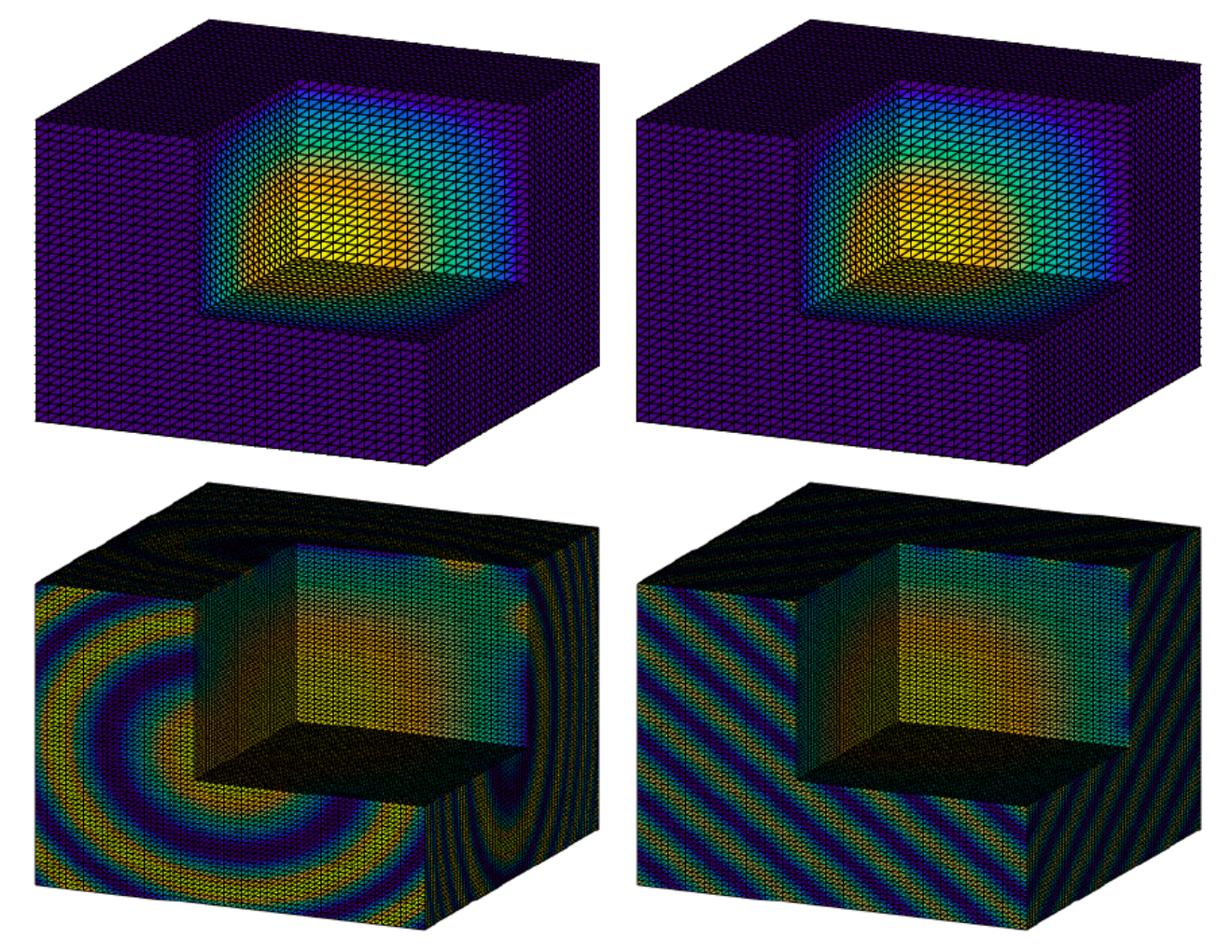
| Case 1 | Case 2 | |
|---|---|---|
5.1 Convergence of the new schemes
First, we look at the convergence rate of both the RBI scheme and the RBCG method, and compare it with that of the conjugate gradient method with and without multigrid as a preconditioner. The histories of convergence for each scheme are reported in Figure 2 and Figure 3. Here, we test the methods at randomly chosen parameter values in their domain and respectively for the two cases, and observe the relative error of residual in norm:
| (22) |
For each scheme, we plot the best and worst case scenario, i.e. the cases that take the largest and smallest number of steps for convergence among all 100 parameter values.
For Case 1, as shown in Figure 2, we report two scenarios, and . We clearly see that, even if we only use a one-dimensional RB as a preconditioner (top row of Figure 2, the method converges in half number of steps. When we raise the dimension of the RB preconditioner to 5, this ratio decreases to . This demonstrates the high level of effectivity of the new scheme. For Case 2, we test the schemes for and . It also demonstrate that the RBI-based schemes vastly outperforms the CG method, while outperforming or matching the multigrid-preconditioned CG methods when it comes to the number of steps toward convergence.
5.2 Computation time
Next, we examine the computation time for each scheme. We show in Figure 4 the cumulative computation time for each scheme as we increase the RB dimension. Of course, the CG and multigrid-preconditioned CG stay the same. For that reason, we use the CG timing as reference. We see that, as the RB dimension increases, the RB schemes becomes more economical going from being more expensive than CG to much less expensive. Comparing with the multigrid-preconditioned CG, we clearly see that, even though the number of steps are only slightly better or comparable as shown in Figures 2 and 3), the RB-based schemes are orders of magnitude more efficient. This of course is because each iteration of the RB schemes is much fast than one iteration of the multigrid-preconditioned CG.
5.3 Impact of the RB dimension on convergence
Here, we would like to examine the impact of the RB dimension on the convergence of the RBI and RBCG schemes. Toward that end, we plot the average of the numbers of steps (defined to be the average of the “best” and “worst” cases shown in Figures 2 and 3) as a function of the RB dimension. This is displayed in Figure 5. We observe that the increase of the RB dimension clearly has a positive impact on the convergence of the schemes.
5.4 Performance for large system
Finally, we test the methods on a large system. Toward that end, we refine the mesh of case until there are more than million degrees of freedom. The results are given in Figure 6. We see that the performance of RBCG is still comparable with the multigrid preconditioned CG in terms of convergence. However, for a large system like this, more levels are necessary for the V-cycle of multigrid. The situation is exacerbated by the storage and application of the multiple large restriction and prolongation operators, especially at the higher levels. As a result, it becomes challenging to apply MG-CG scheme on such systems, as can be seen from the computational time in Figure 6 right. These constraints are substantially mitigated by our RBCG scheme.
6 Conclusion
Inspired by the traditional RB and multigrid methods, we develop and demonstrate a class of reduced basis methods, the first of its kind, for iteratively solving parametrized SPD linear systems. It employs a greedy algorithm to efficiently determine sampling parameters and associated basis vectors and build a system-specific subspace. Based on this subspace, solution procedures are designed to employ the reduced basis approximation as a stand-alone iterative solver or as a preconditioner in the conjugate gradient method. Numerical experiments demonstrate the superiority of the methods both in terms of number of steps toward convergence and the computational cost of each step.
Extension of this novel approach to the non-symmetric and indefinite cases, and to systems resulting from time-dependent problems are a subject of ongoing research. For the RB schemes, the main role of the smoother is to reduce the error rather than smooth it. Hence, the construction of an appropriate smoother for the RB schemes is also worthy of investigation.
References
- [1] M. Barrault, Y. Maday, N. C. Nguyen, and A. T. Patera. An ’empirical interpolation’ method: application to efficient reduced-basis discretization of partial differential equations. Comptes Rendus Mathematique, 339(9):667–672, 2004.
- [2] P. Benner, A. Cohen, M. Ohlberger, and K. Willcox. Model Reduction and Approximation: Theory and Algorithms, volume 15. SIAM, 2017.
- [3] S. Boyaval, C. L. Bris, T. Lelièvre, Y. Maday, N. C. Nguyen, and A. T. Patera. Reduced basis techniques for stochastic problems. Archives of Computational Methods in Engineering, 17:435–454, 2010.
- [4] A. Brandt. Multi-level adaptive solutions to boundary-value problems. Mathematics of computation, 31(138):333–390, 1977.
- [5] S. Brenner and R. Scott. The Mathematical Theory of Finite Element Methods. Springer, New York, NY, 3rd editio edition, dec 2007.
- [6] W. L. Briggs, V. E. Henson, and S. F. McCormick. A multigrid tutorial. SIAM, 2000.
- [7] A. Buffa, Y. Maday, A. T. Patera, C. Prud’homme, and G. Turinici. A priori convergence of the Greedy algorithm for the parametrized reduced basis method. ESAIM: Mathematical Modelling and Numerical Analysis, 46(03):595–603, 2012.
- [8] L. Chen. iFEM: An integrated Finite Element Methods Package in MATLAB. Preprint, University of California at Irvine, Irvine, CA, 2009.
- [9] Y. Chen, S. Gottlieb, and Y. Maday. Parametric Analytical Preconditioning and its Applications to the Reduced Collocation Methods. C. R. Acad. Sci. Paris, Ser. I, 352:661–666, 2014.
- [10] Y. Chen, J. S. Hesthaven, Y. Maday, and J. Rodríguez. Certified Reduced Basis Methods and Output Bounds for the Harmonic Maxwell’s Equations. SIAM Journal on Scientific Computing, 32(2):970–996, jan 2010.
- [11] Y. Chen, J. Jiang, and A. Narayan. Robust residual-based and residual-free greedy algorithms for reduced basis methods. 2017.
- [12] D. Darnell, R. B. Morgan, and W. Wilcox. Deflated GMRES for systems with multiple shifts and multiple right-hand sides. Linear Algebra and Its Applications, 429(10):2415–2434, 2008.
- [13] J. L. Eftang, D. B. Huynh, D. J. Knezevic, and A. T. Patera. A two-step certified reduced basis method. Journal of Scientific Computing, 51(1):28–58, 2012.
- [14] J. L. Eftang, A. T. Patera, and E. M. Rønquist. An ”hp” Certified Reduced Basis Method for Parametrized Elliptic Partial Differential Equations. SIAM Journal on Scientific Computing, 32(6):3170–3200, 2010.
- [15] H. C. Elman and V. Forstall. Preconditioning Techniques for Reduced Basis Methods for Parameterized Elliptic Partial Differential Equations. SIAM Journal on Scientific Computing, 37(5):S177–S194, 2015.
- [16] R. W. Freund and N. M. Nachtigal. QMR: A quasi-minimal residual method for non-hermitian linear systems. Numerische Mathematik, 60(1):315–339, dec 1991.
- [17] A. Frommer and U. Glässner. Restarted GMRES for Shifted Linear Systems. SIAM Journal on Scientific Computing, 19(1):15–26, 1998.
- [18] L. Grammont, N. J. Higham, and F. Tisseur. A framework for analyzing nonlinear eigenproblems and parametrized linear systems. Linear Algebra and Its Applications, 435(3):623–640, 2011.
- [19] M. A. Grepl, Y. Maday, N. C. Nguyen, and A. T. Patera. Efficient reduced-basis treatment of nonaffine and nonlinear partial differential equations. Mathematical Modelling And Numerical Analysis, 41(3):575–605, 2007.
- [20] G.˜Rozza, D.B.P.˜Huynh, and A.T.˜Patera. Reduced Basis Approximation and A Posteriori Error Estimation for Affinely Parametrized Elliptic Coercive Partial Differential Equations — Application to Transport and Continuum Mechanics. Arch. Comput. Methods Eng., 15(3):229–275, 2008.
- [21] G. D. Gu and V. Simoncini. Numerical solution of parameter-dependent linear systems. Numerical Linear Algebra with Applications, 12(9):923–940, 2005.
- [22] W. Hackbusch. Multi-grid methods and applications, volume 4. Springer Science & Business Media, 2013.
- [23] M. Hestenes and E. Stiefel. Methods of conjugate gradients for solving linear systems. Journal of Research of the National Bureau of Standards, 49(6):409 – 436, 1952.
- [24] J. S. Hesthaven, G. Rozza, and B. Stamm. Certified reduced basis methods for parametrized partial differential equations. SpringerBriefs in Mathematics. Springer, Cham; BCAM Basque Center for Applied Mathematics, Bilbao, 2016. BCAM SpringerBriefs.
- [25] M. E. Kilmer and E. De Sturler. Recycling subspace information for diffuse optical tomography. SIAM Journal on Scientific Computing, 27(6):2140–2166, 2006.
- [26] D. Kressner and C. Tobler. Low-rank tensor Krylov subspace methods for parametrized linear systems. SIAM Journal on Matrix Analysis and Applications, 32(4):1288–1316, 2011.
- [27] D. J. Mavriplis. Multigrid Strategies for Viscous Flow Solvers on Anisotropic Unstructured Meshes. Journal of Computational Physics, 145(1):141–165, 1998.
- [28] Y. Nesterov. Introductory Lectures on Convex Optimization, volume 87 of Applied Optimization. Springer US, Boston, MA, 2004.
- [29] Y. Nesterov. Smooth minimization of non-smooth functions. Mathematical Programming, 103(1):127–152, dec 2004.
- [30] Y. Nesterov. Gradient methods for minimizing composite functions. Mathematical Programming, 140(1):125–161, dec 2012.
- [31] N. C. Nguyen, P. Fernandez, R. M. Freund, and J. Peraire. Accelerated residual methods for the iterative solution of systems of equations. SIAM J. Sci. Comput., Accepted, 2018.
- [32] C. C. Paige and M. A. Saunders. Solution of sparse indefinite systems of linear equations. SIAM Journal on Numerical Analysis, 12(4):617–629, sep 1975.
- [33] M. L. Parks, E. De Sturler, G. Mackey, D. D. Johnson, and S. Maiti. Recycling Krylov subspaces for sequences of linear systems. SIAM Journal on Scientific Computing, 28(5):1651–1674, 2006.
- [34] C. Prud’homme, D. Rovas, K. Veroy, Y. Maday, A. T. Patera, and G. Turinici. Reliable real-time solution of parametrized partial differential equations: Reduced-basis output bounds methods. Journal of Fluids Engineering, 124(1):70–80, mar 2002.
- [35] G. Rozza, D. B. P. Huynh, and A. T. Patera. Reduced basis approximation and a posteriori error estimation for affinely parametrized elliptic coercive partial differential equations: Application to transport and continuum mechanics. Archives Computational Methods in Engineering, 15(4), 2008.
- [36] Y. Saad and M. H. Schultz. GMRES: A generalized minimal residual algorithm for solving nonsymmetric linear systems. SIAM J. Sci. Stat. Comput., 7:856–869, 1986.
- [37] V. Simoncini and F. Perotti. On the numerical solution of (ˆ2a+b+c),x=b and application to structural dynamics. SIAM Journal on Scientific Computing, 23(6):1875–1897, 2002.
- [38] P. Sonneveld. CGS: A fast Lanczos-type solver for nonsymmetric linear systems. SIAM Journal on Scientific and Statistical Computing, 10(1):36–52, jan 1989.
- [39] H. A. van der Vorst. Bi-CGSTAB: A fast and smoothly converging variant of Bi-CG for the solution of nonsymmetric linear systems. SIAM Journal on Scientific and Statistical Computing, jul 2006.
- [40] K. Veroy and A. T. Patera. Certed real-time solution of the parametrized steady incompressible Navier-Stokes equations: rigorous reduced-basis a posteriori error bounds. Int. J. Numer. Meth. Fluids, 47:773–788, 2005.
- [41] D. Young. Iterative methods for solving partial difference equations of elliptic type. Transactions of the American Mathematical Society, 76(1):92–92, jan 1954.