Network Signatures from Image Representation of Adjacency Matrices: Deep/Transfer Learning for Subgraph Classification
Abstract.
We propose a novel subgraph image representation for classification of network fragments with the targets being their parent networks. The graph image representation is based on 2D image embeddings of adjacency matrices. We use this image representation in two modes. First, as the input to a machine learning algorithm. Second, as the input to a pure transfer learner. Our conclusions from several datasets are that
- •
deep learning using our structured image features performs the best compared to benchmark graph kernel and classical features based methods; and,
- •
pure transfer learning works effectively with minimum interference from the user and is robust against small data.
Keywords:
Deep Learning, Network Signatures, Graph Classification, Image Embeddings of Graphs1. Introduction
With the advent of big data, graphical representation of information has gained popularity. Being able to classify graphs has applications in many domains. We ask (Figure 1), “Given a small piece of a parent network, is it possible to identify the parent network?”
We address this problem using structured image representations of graphs.
8,8)
Adjacency matrices are notoriously bad for machine learning. It is easy to see why, from the unstructured image of a small fragment of a road network, in Figure (a) below. Though the road network is structured, the random image would convey little or no information to machine learning algorithms (in the image, a black pixel at position corresponds to an edge between nodes and ).
| (a) Unstructured image of adjacency matrix (road network) | ![[Uncaptioned image]](1804.06275v1/road_unsorted.png) |
| (b) Structured image of adjacency matrix (road network) | ![[Uncaptioned image]](1804.06275v1/road_sorted.png) |
Reordering the vertices (Figure (b) above) gives a much more structured image for the same subgraph as in (a). Now, the potential to learn distinguishing properties of the subgraph is evident. We propose to exploit this very observation to solve a basic graph problem (see Figure 1). The datasets mentioned in Figure 1 are discussed in Section 2.4.
We stress that both images are lossless representations of the same adjacency matrix. We use the structured image to classify subgraphs in two modes:
(i) Deep learning models on the structured image representation as input. (ii) The structured image representation is used as input to a transfer learner (Caffe: see Section 2.3) in a pure transfer learning setting without any change to the Caffe algorithm. Caffe outputs top- categories that best describe the image. For real world images, these Caffe-descriptions are human friendly as seen in Figure 2(a). However, for network-images, Caffe gives a description which doesn’t really have intuitive meaning (Figure 2(b)). We map the Caffe-descriptions to vectors. This allows us to compute similarity between network images using the similarity between Caffe description-vectors (see Section 2).
| Classification | Score |
|---|---|
| Pug | 0.75 |
| Bull Mastiff | 0.13 |
| Brabancon Giffon | 0.04 |
| French Bulldog | 0.02 |
| Muzzle | 0.01 |

| Classification | Score |
|---|---|
| Window Screen | 0.29 |
| Digital Clock | 0.07 |
| Window Shade | 0.06 |
| Scoreboard | 0.05 |
| Oscilloscope | 0.04 |
1.1. Our Contributions
The essential difference between our work and previous approaches is that we transform graph classification into image classification. We propose an image representation of the adjacency matrix as input to machine learning algorithms for graph classification, yielding top performance. We further show that this representation is powerful enough to serve as input to a pure transfer learner that has been trained in a completely unrelated image domain.
The Adjacency Matrix Image Representation. Given a sample subgraph from a parent network, the first step is to construct the image representation. We illustrate the workflow below.
14,3)
We use the novel method proposed in (Wu et al., 2016) which produces an adjacency matrix that is invariant to permutations of the vertices in the adjacency matrix. The image is simply a “picture” of this permutation-invariant adjacency matrix.
Deep Learning Using Adjacency Matrix Images. We train deep image classifiers (see Section 2.2) on our structured image representation as shown below. We compared several methods, including graph kernel classifiers and classifiers based on standard topological features. Our image representation performs best.
13,1.6)
Transfer Learning Using Adjacency Matrix Images. When data is scarce or there are many missing labels, a popular option is transfer learning to leverage knowledge from some other domain. Typically the other domain is closely related to the target application. It is unusual for learning in a completely unrelated domain to be transferable to a new target domain. We show that our image representation is powerful enough that one can directly transfer learn from the real world image domain to the network domain (two completely unrelated domains). That is, our image representation provides a link between these two domains enabling classification in the graph domain to leverage the wealth of techniques available to the image domain.
The image domain has mature pre-trained models based on massive data. For example, the open-source Caffe deep learning framework is a convolutional neural network trained on the ImageNet data which can recognize everyday objects like chairs, cats, dogs etc. ((Krizhevsky et al., 2012)). We use Caffe as is. Caffe is a black box that provides a distribution over image classes which we refer to as the Caffe-classification vector. The Caffe results are then mapped back into the source domain using a distance-based heuristic e.g. Jaccard distance and -nearest neighbors as shown below.
13,1.6)
Images, not graphs, are passed through the Caffe deep neural network, and as we shall show, one can get good performance from as little as 10% of the training data used in the ab initio machine learning approach. It is quite stunning that such little training data together with un-tweaked transfer learning from a completely unrelated domain can perform so well. The reason is that our image representation provides very structured images (human-recognizable) for real world networks. Though these images are not traditional images like those used in training Caffe, Caffe still maps the different structured images to different distributions over its known classes, hence we are able to transfer this knowledge from Caffe to graph classification.
1.2. Related Work
(Wu et al., 2016) introduced the problem we study: Can one identify the parent network from a small subgraph? How much does local information reveal about the parent graph globally? Our approach is from the supervised setting and the unsupervised transfer learning setting.
There is previous work on similar problems using graph kernels, (Kashima and Inokuchi, 2002; Kashima et al., 2003; Kudo et al., 2004), which use kernels to compute similarities between graphs and then algorithms like SVM for classification. Choosing kernels is not straightforward and is certainly not “one-size-fits-all”. Further, these kernel methods do not scale well for very large graphs. We compare with one such method proposed by (Shervashidze et al., 2011).
Some approaches construct features from topological attributes of the subgraph ((Li et al., 2011)). Topological properties of social networks have been extensively studied by (Ahn et al., 2007; Ferrara and Fiumara, 2012; Sridharan, 2011). The challenges are that it is difficult to come up with a “master set” of features that can be used to represent graphs from different domains. For example, assortativity could be an important feature in social networks while being of little significance in road networks. It is hard to identify beforehand what features need to be computed for a given problem, thus leading to a trial and error scenario. Nevertheless, we still compare with classical features trained with logistic regression.
Transfer learning is useful when a classification task in one domain can leverage knowledge learned in a related domain (see (Pan and Yang, 2010) for an extensive survey). (Raina et al., 2007) introduced a method called self-taught learning which takes advantage of irrelevant unlabeled data to boost performance. (Zhu et al., 2011) discuss heterogeneous transfer learning where they use information from text data to improve image classification performance. (Quattoni et al., 2008) create a new representation from kernel distances to large unlabeled data points before performing image classification using a small subset of reference prototypes.
Paper Organization.
2. Methodology
Given fragments of a large network we first obtain their structured images to construct the training examples. In the supervised setting, we learn the final classifier from this training. In the transfer setting, we use the Caffe framework as a black-box to obtain the label-vectors. To classify a test subgraph, we first obtain its label-vector through Caffe, compute the distance between the test label-vector and the training label-vectors, and classify using majority among the nearest training examples. We now give the details.
2.1. Image embeddings of graphs
An adjacency matrix of a graph can be thought of as a monochrome image with 1s corresponding to dark pixels and 0s corresponding to white pixels. This observation, however, is of limited practical use since it is unstructured and not permutation invariant. We suitably reorder the vertices in the graph so that structural information can be represented by spatial organization within the image. We utilize a novel technique for producing a permutation-invariant ordering of the adjacency matrix, first given in (Wu et al., 2016). The authors describe several ways to sort an adjacency matrix like page rank, degree based sorting, etc. They show that the BFS-like approach works best. The ordering starts with the node of highest degree (ties are broken using -neighborhood size for , then , ). Subsequently, the ordering proceeds based on a combination of shortest paths and degrees. Details can be found in (Wu et al., 2016). The ordering scheme results in permutation-invariant adjacency matrices from which we obtain structured images.
We observe that the image embeddings have enough structure so that even the human eye can distinguish between different networks without much effort. Neural networks are highly successful in recognizing real world objects that have high level structural similarity. For example, all dogs have similar features although they are individually different. Similarly, the image embeddings of all road network subgraphs “look" similar but are microscopically different. From a neural network’s perspective, the structured image embeddings are like any other images. The fact that these structured image embeddings were obtained from adjacency matrices has no methodological impact on the neural network model.
2.2. Network Signatures from Deep Learning
Our primary objective is to use deep learning to learn to classify subgraphs into their parent networks using our image representation of the subgraph. However, we also tested a wide variety of other methods as well. We describe them briefly below.
Deep Belief Network (DBN). Our DBNs (see: (Hinton, 2009)) have multiple layers of unsupervised Restricted Boltzmann Machines (RBMs), (Hinton et al., 2006), trained greedily and fine-tuned using back-propagation.
Typically, DBNs have an input layer, hidden layer(s) and a final output layer. For an image, the input layer has 64 nodes. The hidden layers consist of RBMs where the output of each of RBMs are used as input to the next. Finally, the output layer contains a node for each class. The probabilities of each class label is returned. The one with the highest probability is chosen as the overall classification for the given input.
Convolutional Neural Network (CNN). CNNs (cnnkeras) have proven to be very effective in real world image classification tasks. The building blocks of a CNN are convolution layers, non-linear layers such as Rectified Linear Units (ReLU), pooling layers and fully connected layers for classification.
Stacked De-Noising Auto-Encoder (SdA). We used the stacked de-noising auto-encoder (SdA) based on greedy training presented in (Wu and Magdon-Ismail, 2016). In a regular multi-layer deep neural network, each layer is trained to "reconstruct" the input from the previous layer. Then, the system is fine tuned by using back-propagation. In SdA, instead of the original input, a noisy input is fed to the system.
Diffusion-Convolutional Neural Network (DCNN). DCNNs introduced by (Atwood and Towsley, 2016), work on the graphs themselves rather than the image embeddings of their adjacency matrices. DCNNs provide a flexible tool for of graphical data that encodes node features, edge features, and purely structural information with little preprocessing. DCNNs learn diffusion-based representations from graph-structured data using a diffusion-convolution operation.
Graph Kernels (GK). We use the graph kernel in (Shervashidze et al., 2011) which extracts features based on the Weisfeiler-Lehman test of isomorphism on graphs. It maps the original graph to a sequence of graphs, whose node attributes capture topological and label information. We use the implementations from (Ghisu, [n. d.]).
Classical Features and Logistic Regression (LR). We compute 15 classic features on subgraphs and train a logistic regression model (sklearnlogreg) on these features. Our features are: transitivity, average clustering co-efficient, average node connectivity, edge connectivity, average eccentricity, diameter, average shortest path, average degree, fraction of single-degree nodes, average closeness centrality, central points, density, average neighbor degree and top two eigen values of the adjacency matrix.
All methods were tested in a standard supervised learning framework where training examples are given (inputs and targets ) DBN, CNN and SdA, the input is our image representation of the subgraph. For DCNN and GK, the input is the graph itself. For LR, the input is a vector of 15 classical features.
2.3. Caffe-Classification and Transfer Learning
Caffe (Jia et al., 2014) is a large scale project developing a deep learning framework for image classification. It has been extensively used in image classification and filter visualization, learning handwritten digits and style recognition, etc. (Benanne, 2014). We use a pre-trained model that is trained on a crowd-sourced labeled data set ImageNet. As of 2016, ImageNet had more than 10 million hand-annotated images. The massive volume combined with a deep convolutional neural network gives us fine-grained discriminatory power for images.
Given an image, Caffe gives a vector of (label, label-probability) tuples. An example of the output for a real image is shown in Figure 2(a). Although Caffe has not been trained on image embeddings of graphs, such images nonetheless produce vectors that have sufficient discriminatory information that we extract using the post processing step (see Section 2.3.1). An example of a vector corresponding to a Facebook subgraph is shown in Figure 2(b).
Caffe provides either maximally accurate or maximally specific classification. We use the maximally specific option. Further, while we have shown cardinality-5 vectors for brevity in Figure 2, we use cardinality-10 vectors in our experiments.
Finally, Caffe is trained on color images, while our images are black and white (each pixel represents presence or absence of an edge). Embeddings that encode additional information (e.g. edge weights) as RGB values may allow us to leverage the color capability of Caffe, which is a possible avenue for future research.
2.3.1. Post-processing for Graph Classification
Caffe provides a set of label vectors for each training network . Each labelvector is a tuple of (label, label-probability pairs) as deemed by Caffe. In this work, we ignore the probabilities, and treat each vector as an unordered list of labels (strings). Each training vector also has a ground truth parent label.
We use Jaccard similarity to compute a similarity metric between two label-vectors and :
We leave for future work the use of more sophisticated metrics which could use the probabilities from Caffe - our goal is to demonstrate the potential of even this simplest possible approach.
For a test graph, we get the label-vector from Caffe and then compute the nearest training vectors using the Jaccard distance to each training vector and classify using the majority class among these nearest training vectors (ties are broken randomly). The test example is correctly classified if and only if its ground truth matches . One advantage of the nearest neighbor approach is that it seamlessly handles multiclass problems.
2.4. Data
We used a variety of parent graphs, from citation networks to social networks to e-commerce networks (see Table 1 and the Appendix). Our classifiers learn network-signatures from the image representations. To gain insight into these network signatures, we show the top principal component from each network class in Figure 4(a). To get these principal components, we used a PCA analysis of the vectorized images in each class (similar to (Turk and Pentland, 1991)).
In Figure 4(b), we show the structured images of specific 64-node subgraphs from each class. These are adjacency matrices that have gone through the structuring process described in Section 2.1. Observe that the images for different classes are both well structured and quite different from each other. This is why learning is able to perform well at classifying the subgraphs, see in Section 3.
 (a)
(a)
 (b)
(b)
 (c)
(c)
 (d)
(d)
 (e)
(e)
 (f)
(f)
 (g)
(g)
 (h)
(h)
 (i)
(i)
 (a)
(a)
 (b)
(b)
 (c)
(c)
 (d)
(d)
 (e)
(e)
 (f)
(f)
 (g)
(g)
 (h)
(h)
 (i)
(i)
| Dataset | # Nodes | # Edges | Reference(s) |
| Citation | 34,546 | 421,578 | (Leskovec et al., 2005; Gehrke et al., 2003) |
| 4039 | 88,234 | (Leskovec and Mcauley, 2012) | |
| Road Network | 1,088,092 | 1,541,898 | (Leskovec et al., 2009) |
| Web | 875,713 | 5,105,039 | (Leskovec et al., 2009) |
| Wikipedia | 4,604 | 119,882 | (West and Leskovec, 2012; West et al., 2009) |
| Amazon | 334,863 | 925,872 | (Leskovec et al., 2007) |
| DBLP | 317,080 | 1,049,866 | (Yang and Leskovec, 2012) |
| Terrorist Net. | 271 | 756 | (JJATT, 2009) |
| Gowalla | 196,591 | 950,327 | (Cho et al., 2011) |
3. Experimental Setup and Results
We now describe our experimental setup and present the results from the supervised and transfer approaches.
3.1. Deep Supervised Image Classifiers
We perform graph classification for the above mentioned parent networks. We perform a random walk on each of these networks times until we get the desired number of nodes for a training subgraph, denoted by . We tried , , . So, with networks and samples per network, we create datasets with samples each. Each dataset is of the size .
For a given dataset, we randomly chose of it for training, validation and testing respectively. The accuracy score is defined as the ratio of the sum of the principal diagonal entries of the confusion matrix over the sum of all the entries of the confusion matrix (sometimes called the error matrix (Stehman, 1997)). We report the accuracy score for each classifier for in the following table. The full confusion matrices are in the Appendix.
| CNN | SdA | DBN | DCNN | GK | LR | |
| Acc. | 0.86 | 0.79 | 0.81 | 0.45 | 0.73 | 0.83 |
CNN was the best performing classifier while DCNN and GK11 1 It uses libsvm’s (chang2011libsvm) “one-vs-one” method for multiclass classification were the poorest performers. Off-the-shelf deep learning with our graph image features is the top performer. Figure 5 summarizes the performance of all the methods. As expected, we obtained higher accuracy as the subgraph size increases, because the subgraph contains more information (the flat line in Figure 5 is for random guessing). We point out that even with node subgraphs do significantly better than random.
We also note that although LR performs well, it is very hard to choose the features when graphs come from different domains. One set of features that worked best in one scenario may not be the best in another. So, off-the-shelf CNN, DBN or SdA with our image features are an easy choice to make as they require little effort and deliver top performance. We also considered hybrid training sets with subgraphs of different sizes. We observed that the performance was better when the mixture had more examples with higher . This is inline with the results in Figure 5. Interested readers can refer to the Appendix for more details.
Graph kernel and feature-based methods performed better than DCNN, but not as well as the image embedding based methods. Kernel methods are complex and usually slow and the fact that they did not perform spectacularly do not make them attractive. One may notice that the accuracy scores for LR are very comparable to SdA. However, we would like to remark that LR is a lossy method since it approximates the graph and boils it down to a handful of features. It is very hard to decide which features must be used and the choice may vary for graphs in different domains in order to get optimal results. However, our approach is completely lossless. The structured image representation of the graph has every bit of the information the adjacency matrix does. So, we would not have to make any compromises to get the best out of the data.

Out of the 4 neural network classification models, DCNN is the only one that takes a graph as an input instead of images. In fact, it takes two inputs: an adjacency matrix and a design matrix. Design matrix takes information (average degree, clustering co-efficient etc.) about each node in the adjacency matrix. We observed no change in performance when we did not provide any information in the design matrix. This is because these accessory properties can be calculated from the graph which is already an input. The neural network is expected to have learned these features already.
3.2. Transfer Learning
We present our experimental results for transfer learning. We show that our transfer learning approach is highly resilient to sparse training data. We achieve a respectable accuracy even when only 10% of the data was used for training.
We treat Caffe as a black-box that requires for transfer learning. Transfer learning helps because when one does not have access to ample data to train classifiers from scratch.
We did the following experiments: (a) differentiating networks of similar theme/type (i. Terrorist Net. vs Facebook, ii. Citation vs DBLP and iii. Web vs Wiki); and (b) full multiclass classification. Tables 2(a), 2(b), and 2(c) show the results of classification between similarly-themed networks. We see varying degrees of success: Wiki vs Web gives a very high accuracy of 95%. The other two are respectable as well, with 90% and 80% accuracies.
| Data | Prc. | Rec. | F1 |
|---|---|---|---|
| Ter. Net. | 0.84 | 0.99 | 0.91 |
| FB | 0.99 | 0.81 | 0.89 |
| Acc. | 90.3% | ||
| Data | Prc. | Rec. | F1 |
|---|---|---|---|
| Cit. | 0.90 | 0.67 | 0.76 |
| DBLP | 0.74 | 0.92 | 0.82 |
| Acc. | 79.51% | ||
| Data | Prc. | Rec. | F1 |
|---|---|---|---|
| Wiki | 0.96 | 0.93 | 0.94 |
| Web | 0.93 | 0.97 | 0.94 |
| Acc. | 94.57% | ||
Table 3 shows that transfer learning does not do quite as well when it comes to multiclass classification, which is challenging in general. Our particular approach of using the majority rule may be somewhat more impacted since now the correct class has to outnumber several other classes.
| Data | Prc. | Rec. | F1 |
|---|---|---|---|
| Wiki | 0.71 | 0.79 | 0.75 |
| Web | 0.66 | 0.73 | 0.69 |
| DBLP | 0.57 | 0.59 | 0.58 |
| Terrorist Net. | 0.48 | 0.70 | 0.57 |
| Citations | 0.36 | 0.18 | 0.24 |
| 0.84 | 0.66 | 0.74 | |
| Accuracy | 61% | ||
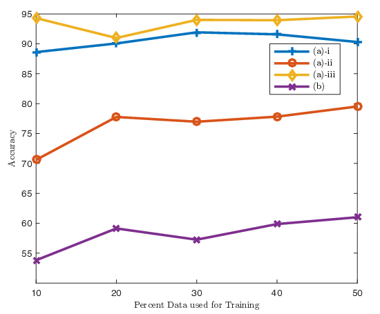
Figure 6 plots the accuracy numbers pairwise classification as we progressively increase the proportion of data used for identifying k-nearest neighbors (the rest of the data is used for testing). The takeaway message is that transfer learning works, and is robust to small training data. Even 10% of the data gives good performance. Most learning techniques, especially deep neural networks are sensitive to training data size. The relative insensitivity of transfer learning is because it leverages a pre-trained recognition engine in the image domain which has already been trained with a massive dataset. Hence transfer learning approach is very robust and resilient to sparse training data.
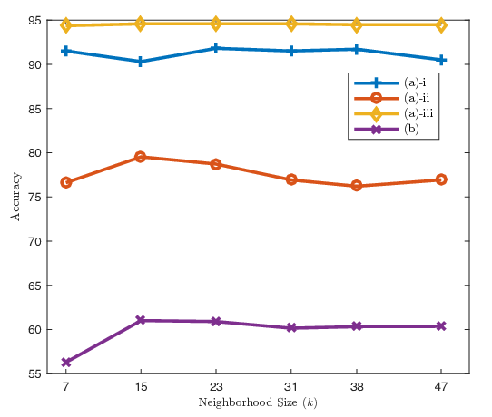
Finally, we study the impact of , the neighborhood size for the majority rule. The details are in the Appendix, but the take away fact is that as long as , the performance is robust to .
4. Conclusion and Future Work
Our experiments overwhelmingly show that our structured image representation of graphs achieves successful graph classification with ease. The image representation is lossless, that is the image embeddings contain all the information in the corresponding adjacency matrix. Our results also show that even with very small subgraphs, deep network models are able to extract network signatures from our highly structured images. Specifically, with just 64-node subgraphs from networks with up to 1 million nodes, we were able to predict the parent network with accuracy. Even with 8-node subgraphs, accuracies are significantly better than random. Further, we demonstrated that the image embedding approach provides many advantages over graph kernel and feature-based methods.
We also presented an approach to graph classification using transfer learning from a completely different domain. Our approach converts graphs into 2D image embeddings and uses a pre-trained image classifier (Caffe) to obtain label-vectors. In a range of experiments with real-world data sets, we have obtained accuracies from 70% to 94% for pairwise classification and 61% for multiclass classification. Further, our approach is highly resilient to training-to-test ratio, that is, can work with little training data. Our results show that such an approach is very promising, especially for applications where training data is not readily available (e.g. terrorist networks).
Future work includes improvements to the transfer learning by improving the distance function between label-vectors, as well as using the probabilities from Caffe. Further, we would also look to generalize this approach to other domains, for example classifying radio frequency map samples using transfer learning.
Acknowledgments. This research was supported by the Army Research Laboratory under Cooperative Agreement W911NF-09-2-0053 (the ARL-NSCTA). The views and conclusions contained in this document are those of the authors and should not be interpreted as representing the official policies, either expressed or implied, of the Army Research Laboratory or the U.S. Government. The U.S. Government is authorized to reproduce and distribute reprints for government purposes notwithstanding any copyright notation here on.
References
- Ahn et al. (2007) Yong-Yeol Ahn, Seungyeop Han, Haewoon Kwak, Sue Moon, and Hawoong Jeong. 2007. Analysis of Topological Characteristics of Huge Online Social Networking Services. WWW (2007).
- Atwood and Towsley (2016) James Atwood and Don Towsley. 2016. Diffusion-convolutional neural networks. NIPS (2016).
- Benanne (2014) Benanne. 2014. https://www.reddit.com/2c9x0s. (2014).
- Cho et al. (2011) Eunjoon Cho, Seth A Myers, and Jure Leskovec. 2011. Friendship and mobility: user movement in location-based social networks. KDD (2011).
- Ferrara and Fiumara (2012) Emilio Ferrara and Giacomo Fiumara. 2012. Topological Features of Online Social Networks. CoRR (2012).
- Gehrke et al. (2003) Johannes Gehrke, Paul Ginsparg, and Jon Kleinberg. 2003. Overview of the 2003 KDD Cup. SIGKDD Explor. Newsl. (2003).
- Ghisu ([n. d.]) Elisabetta Ghisu. [n. d.]. https://github.com/BorgwardtLab/Graph-Kernel-Suite. ([n. d.]).
- Hinton (2009) G. E. Hinton. 2009. Deep belief networks. Scholarpedia (2009).
- Hinton et al. (2006) Geoffrey E Hinton, Simon Osindero, and Yee-Whye Teh. 2006. A fast learning algorithm for deep belief nets. Neural computation (2006).
- Jia et al. (2014) Yangqing Jia, Evan Shelhamer, Jeff Donahue, Sergey Karayev, Jonathan Long, Ross Girshick, Sergio Guadarrama, and Trevor Darrell. 2014. Caffe: Convolutional architecture for fast feature embedding. In Proceedings of the 22nd ACM international conference on Multimedia. ACM, 675–678.
- JJATT (2009) JJATT. 2009. http://doitapps.jjay.cuny.edu/jjatt/data.php. (2009).
- Kashima and Inokuchi (2002) Hisashi Kashima and Akihiro Inokuchi. 2002. Kernels for Graph Classification. International Workshop on Active Mining (2002).
- Kashima et al. (2003) Hisashi Kashima, Koji Tsuda, and Akihiro Inokuchi. 2003. Marginalized kernels between labeled graphs. ICML (2003).
- Krizhevsky et al. (2012) Alex Krizhevsky, Ilya Sutskever, and Geoffrey E Hinton. 2012. Imagenet classification with deep convolutional neural networks. NIPS (2012).
- Kudo et al. (2004) Taku Kudo, Eisaku Maeda, and Yuji Matsumoto. 2004. An Application of Boosting to Graph Classification. NIPS (2004).
- Leskovec et al. (2007) Jure Leskovec, Lada A Adamic, and Bernardo A Huberman. 2007. The dynamics of viral marketing. TWEB (2007).
- Leskovec et al. (2005) Jure Leskovec, Jon Kleinberg, and Christos Faloutsos. 2005. Graphs over Time: Densification Laws, Shrinking Diameters and Possible Explanations. KDD (2005).
- Leskovec et al. (2009) Jure Leskovec, Kevin J Lang, Anirban Dasgupta, and Michael W Mahoney. 2009. Community structure in large networks: Natural cluster sizes and the absence of large well-defined clusters. Internet Mathematics (2009).
- Leskovec and Mcauley (2012) Jure Leskovec and Julian J. Mcauley. 2012. Learning to Discover Social Circles in Ego Networks. NIPS (2012).
- Li et al. (2011) Geng Li, Murat Semerci, Bulent Yener, and Mohammed J Zaki. 2011. Graph classification via topological and label attributes. MLG (2011).
- Pan and Yang (2010) Sinno Jialin Pan and Qiang Yang. 2010. A survey on transfer learning. IEEE Transactions on knowledge and data engineering 22, 10 (2010), 1345–1359.
- Quattoni et al. (2008) Ariadna Quattoni, Michael Collins, and Trevor Darrell. 2008. Transfer learning for image classification with sparse prototype representations. CVPR (2008).
- Raina et al. (2007) Rajat Raina, Alexis Battle, Honglak Lee, Benjamin Packer, and Andrew Y Ng. 2007. Self-taught learning: transfer learning from unlabeled data. ICML (2007).
- Shervashidze et al. (2011) Nino Shervashidze, Pascal Schweitzer, Erik Jan van Leeuwen, Kurt Mehlhorn, and Karsten M Borgwardt. 2011. Weisfeiler-lehman graph kernels. JMLR (2011).
- Sridharan (2011) Ajay Promodh Sridharan. 2011. Topological features of online social networks. University of Victoria (2011).
- Stehman (1997) Stephen V Stehman. 1997. Selecting and interpreting measures of thematic classification accuracy. Remote sensing of Environment (1997).
- Turk and Pentland (1991) Matthew A Turk and Alex P Pentland. 1991. Face recognition using eigenfaces. CVPR (1991).
- West and Leskovec (2012) Robert West and Jure Leskovec. 2012. Human Wayfinding in Information Networks. WWW (2012).
- West et al. (2009) Robert West, Joelle Pineau, and Doina Precup. 2009. Wikispeedia: An Online Game for Inferring Semantic Distances Between Concepts. IJCAI (2009).
- Wu and Magdon-Ismail (2016) Ke Wu and Malik Magdon-Ismail. 2016. Node-By-Node Greedy Deep Learning for Interpretable Features. arXiv preprint arXiv:1602.06183 (2016).
- Wu et al. (2016) Ke Wu, Philip Watters, and Malik Magdon-Ismail. 2016. Network classification using adjacency matrix embeddings and deep learning. ASONAM (2016).
- Yang and Leskovec (2012) Jaewon Yang and Jure Leskovec. 2012. Defining and evaluating network communities based on ground-truth. ICDM (2012).
- Zhu et al. (2011) Yin Zhu, Yuqiang Chen, Zhongqi Lu, Sinno Jialin Pan, Gui-Rong Xue, Yong Yu, and Qiang Yang. 2011. Heterogeneous Transfer Learning for Image Classification. AAAI (2011).
Appendix A Appendix
A.1. Deep Supervised Image Classifiers Results Contd.
We present the confusion matrices of all classifiers for 64-node subgraphs in Table 4. A confusion matrix is such that is equal to the number of observations known to be in class but predicted (confused) to be in class .
A.2. Hybrid Datasets
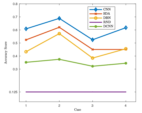
We present the detailed results for different mixtures of datasets that we experimented with in the supervised setting. Although the performance deteriorates when different ’s are mixed, the relative ordering of the methods w.r.t. their performances remains the same. Table below shows the 4 cases and as Figure 7 shows, classification accuracy increases as the contribution by subgraphs with higher increases.
| Nodes | Case 1 | Case 2 | Case 3 | Case 4 |
|---|---|---|---|---|
| 8 | 25% | 10% | 40% | 10% |
| 16 | 25% | 20% | 30% | 40% |
| 32 | 25% | 30% | 20% | 40% |
| 64 | 25% | 40% | 10% | 10% |
A.3. Transfer Learning Results Contd.
Figure 8 shows the variation of accuracy results when is varied in steps of 8 from to , with the base case used for the tabulated results above included for comparison. As can be seen, except for a couple of cases with providing a somewhat lower accuracy, the variation is within 1% of the base case. Thus, as long as , we do not have to worry too much about tuning , showing that the approach is robust.
A.4. Datasets
Citation. This citation network is from Arxiv HEP-PH (high energy physics phenomenology). If a paper cites paper , the graph contains a directed edge from to . There are nodes with edges. See: (Leskovec et al., 2005; Gehrke et al., 2003)
Facebook. This social network contains "friends lists" from Facebook. There are people (nodes) and there is an undirected edge between nodes if they are friends. There are such edges. See: (Leskovec and Mcauley, 2012)
Road Network. This is a road network of Pennsylvania. Intersections and endpoints are represented by nodes, and the roads connecting these intersections are represented by undirected edges. There are nodes and edges in this network. See: (Leskovec et al., 2009)
Web. Nodes in this network represent web pages and directed edges represent hyperlinks between them. There are nodes and edges. See: (Leskovec et al., 2009)
Wikipedia. This is a Wikipedia hyperlink graph. A condensed version of Wikipedia was used in the collection of this dataset. There are articles (nodes) with links (edges) between them. See: (West and Leskovec, 2012; West et al., 2009)
Amazon. This is a product co-purchase network of amazon.com. The nodes are products sold on amazon.com. There is an undirected edge between two products if they are frequently co-purchased. There are nodes and edges. See: (Leskovec et al., 2007)
DBLP. This is a co-authorship network. It has authors for its nodes and there is an undirected edge between them if they have co-authored at least one paper. There are nodes and edges. See: (Yang and Leskovec, 2012)
Terrorist Network. We use the “Al Qaeda Operations Attack Series 1993-2003, Worldwide" dataset consisting of nodes (participants of Al Qaeda terrorist group) with links between them. See: (JJATT, 2009)
Gowalla. Gowalla was a location-based social networking website where users shared their locations by checking-in. The friendship network is undirected and consists of nodes and edges. See: (Cho et al., 2011)
Citation Facebook Road Net. Web Wikipedia Amazon DBLP Terrorist Net. Gowalla Citation 1110 17 2 6 58 292 42 0 139 Facebook 11 1649 0 1 0 5 1 0 0 Road Net. 0 0 1666 0 0 1 0 0 0 Web 39 8 0 1392 1 69 41 0 117 Wikipedia 28 0 0 0 1627 1 0 0 10 Amazon 248 2 4 42 1 1177 74 1 117 DBLP 34 3 0 12 3 82 1513 0 20 Terrorist Net. 3 0 0 0 0 18 14 1632 0 Gowalla 225 5 1 41 48 128 27 0 1192 (a) CNN Citation Facebook Road Net. Web Wikipedia Amazon DBLP Terrorist Net. Gowalla Citation 804 28 0 64 135 369 90 18 158 Facebook 9 1625 0 24 0 1 7 1 0 Road Net. 0 0 1667 0 0 0 0 0 0 Web 49 51 0 1268 17 104 44 1 133 Wikipedia 40 0 0 1 1568 5 1 0 51 Amazon 223 0 0 69 15 997 169 13 180 DBLP 44 29 0 31 3 155 1364 8 33 Terrorist Net. 10 0 0 0 0 51 20 1586 0 Gowalla 199 7 0 124 129 170 42 1 995 (b) SdA Citation Facebook Road Net. Web Wikipedia Amazon DBLP Terrorist Net. Gowalla Citation 1010 20 1 40 87 271 80 0 157 Facebook 9 1626 0 20 0 0 11 0 1 Road Net. 1 0 1665 0 0 1 0 0 0 Web 63 21 0 1353 13 75 32 0 110 Wikipedia 78 0 0 1 1480 5 1 0 101 Amazon 330 2 3 71 12 969 147 3 129 DBLP 54 8 0 27 6 127 1411 1 33 Terrorist Net. 13 0 0 0 0 26 27 1601 0 Gowalla 246 3 0 105 113 161 27 1 1011 (c) DBN Citation Facebook Road Net. Web Wikipedia Amazon DBLP Terrorist Net. Gowalla Citation 192 520 235 12 31 87 479 28 82 Facebook 18 1607 13 10 0 17 1 0 1 Road Net. 0 0 1667 0 0 0 0 0 0 Web 37 297 29 1160 3 32 66 5 38 Wikipedia 163 358 98 0 213 93 710 5 26 Amazon 161 220 347 94 11 126 554 37 116 DBLP 47 282 286 2 31 20 891 34 74 Terrorist Net. 51 9 814 0 26 0 73 694 0 Gowalla 33 224 68 729 34 87 292 2 198 (d) DCNN Citation Facebook Roadnet Web Wikipedia Amazon DBLP Terrorist Net. Gowalla Citation 759 0 0 0 0 907 0 0 0 Facebook 0 1600 0 67 0 0 0 0 0 Roadnet 0 0 1667 0 0 0 0 0 0 Web 0 0 0 1130 0 537 0 0 0 Wikipedia 0 0 0 0 1399 0 0 0 267 Amazon 849 0 0 0 0 817 0 0 0 DBLP 0 0 0 0 0 380 1287 0 0 Terrorist Net. 0 0 0 0 0 190 0 1477 0 Gowalla 790 0 0 0 0 0 0 0 877 (e) GK Citation Facebook Road Net. Web Wikipedia Amazon DBLP Terrorist Net. Gowalla Citation 1095 26 1 35 54 288 44 8 115 Facebook 29 1613 0 20 0 4 1 0 0 Road Net. 0 0 1667 0 0 0 0 0 0 Web 28 44 0 1255 3 66 57 6 208 Wikipedia 5 0 0 0 1656 0 0 0 5 Amazon 214 3 1 87 3 1063 138 42 115 DBLP 18 21 1 17 1 78 1465 31 35 Terrorist Net. 0 0 0 0 0 10 43 1614 0 Gowalla 170 7 1 98 19 62 77 1 1232 (f) LR