A 3-dimensional model of flagellar swimming in a Brinkman fluid
Abstract
We investigate 3-dimensional flagellar swimming in a fluid with a sparse network of stationary obstacles or fibers. The Brinkman equation is used to model the average fluid flow where a flow dependent term, including a resistance parameter that is inversely proportional to the permeability, models the resistive effects of the fibers on the fluid. To solve for the local linear and angular velocities that are coupled to the flagellar motion, we extend the method of regularized Brinkmanlets to incorporate a Kirchhoff rod, discretized as point forces and torques along a centerline. Representing a flagellum as a Kirchhoff rod, we investigate emergent emergent waveforms for different preferred strain and twist functions. Since the Kirchhoff rod formulation allows for out-of-plane motion, in addition to studying a preferred planar sine wave configuration, we also study the case with a preferred helical configuration. Our numerical method is validated by comparing results to asymptotic swimming speeds derived for an infinite-length cylinder propagating planar or helical waves. Similar to the asymptotic analysis for both planar and helical bending, we observe that with small amplitude bending, swimming speed is always enhanced relative to the case with no fibers in the fluid (Stokes) as the resistance parameter is increased. For regimes not accounted for with asymptotic analysis, i.e., large amplitude planar and helical bending, our model results show a non-monotonic change in swimming speed with respect to the resistance parameter; a maximum swimming speed is observed when the resistance parameter is near one. The non-monotonic behavior is due to the emergent waveforms; as the resistance parameter increases, the swimmer becomes incapable of achieving the amplitude of its preferred configuration. We also show how simulation results of slower swimming speeds for larger resistance parameters are actually consistent with the asymptotic swimming speeds if work in the system is fixed.
keywords
Authors should not enter keywords on the manuscript, as these must be chosen by the author during the online submission process and will then be added during the typesetting process (see http://journals.cambridge.org/data/relatedlink/jfm-keywords.pdf for the full list)1 Introduction
Microorganisms such as spermatozoa make forward progression by propagating bending along their flagellum. The emergent flagellar curvature and beat frequency depends on the fluid properties as well as the chemical concentrations within the flagellum (Gaffney et al., 2011; Miki, 2007; Smith et al., 2009b; Suarez & Pacey, 2006; Woolley & Vernon, 2001). The fluid environment experienced by mammalian sperm includes complex geometries and background flows due to interactions with other sperm, cilia, and walls (Fauci & Dillon, 2006; Ho & Suarez, 2001; Suarez & Pacey, 2006; Suarez, 2010). As a sperm progresses toward the egg, the fluid could contain differing amounts of uterine cells, sulfomucins, protein networks and other macromolecules, especially at different times in the menstrual cycle (Katz & Berger, 1980; Katz et al., 1989; Mattner, 1968; Suarez, 2010). Many experiments have examined sperm motility in gels such as methylcellulose (MC) or polyacrylamide (PA), which may be more representative of the in vivo environment. In experiments, the emergent beat frequency and wavelength varied with viscosity in MC gels (Smith et al., 2009b) and the swimming speed of mouse sperm decreased in both MC and PA gels (relative to the culture medium) (Suarez & Dai, 1992). This motivates the development of a 3-dimensional (3D) framework to study emergent properties (e.g., waveform or swimming speed) of a sperm when coupled with this protein network.
Previous computational studies of finite-length swimmers in a Newtonian fluid with preferred bending kinematics have identified that there is a non-monotonic relationship between emergent swimming speeds and bending amplitude (Elgeti et al., 2010; Fauci & McDonald, 1995; Olson & Fauci, 2015). On the other hand, for infinite-length flagella with prescribed bending, the asymptotic swimming speeds are an increasing function with respect to the bending amplitude (Taylor, 1951; Taylor, 1952). Since most gels and biological fluids contain proteins and other macromolecules, recent studies have focused on swimmers in complex fluids. In fluids that exhibit contributions from viscous and elastic effects, the swimming speeds of infinite-length flagella with prescribed kinematics decrease in comparison to the Newtonian case (Fu et al., 2009; Lauga, 2007). In contrast, swimming speeds increase for certain parameter choices for a finite-length swimmer in a nonlinear viscoelastic fluid and a Carreau fluid (Newtonian fluid with shear-dependent viscosity) (Montenegro-Johnson et al., 2012; Teran et al., 2010; Thomases & Guy, 2014). An enhancement in swimming speed relative to a Newtonian fluid has also been observed in a model of a two-phase fluid for a gel when the elastic network is stationary (Fu et al., 2010).
The average fluid flow through an array of sparse, spherical particles can be modeled via the Brinkman equation (Auriault, 2009; Brinkman, 1947; Durlofsky & Brady, 1987; Howells, 1974; Spielman & Goren, 1968). A flow dependent resistance term accounts for the presence of the particles in the fluid. This type of flow has been studied near boundaries and interfaces (Ahmadi et al., 2017; Feng et al., 1998), as well as being a fluid flow to understand flagellar motility of microorganisms. In the case of an infinite-length flagellum in a Brinkman fluid with prescribed bending, in both 2D and 3D, the swimming speed increases as the resistance parameter increases (Ho et al., 2016; Leshansky, 2009). This increase in swimming speed is an enhancement relative to the Newtonian case; the presence of particles or fibers actually aids in forward progression. In contrast, for a finite-length swimmer with preferred planar bending, there was a non-monotonic relationship between swimming speed and the resistance parameter (Cortez et al., 2010; Olson & Leiderman, 2015; Leiderman & Olson, 2016).
To explore emergent properties of flagellar swimming in a fluid with a sparse and stationary protein network, we use the incompressible Brinkman equations to govern the fluid motion (Brinkman, 1947; Howells, 1974):
| (1) | |||||
| (2) |
Here, is the average fluid pressure (force per area), u is the average fluid velocity (length per time), represents the body force (force per unit volume) applied on the fluid by the immersed structure, is the viscosity (force time per area), and is the resistance parameter (inverse length), which is assumed constant (isotropic) and inversely proportional to the square root of the permeability . One can think of the Brinkman equation as the addition of a lower-order resistance term to the Stokes equations for low Reynolds number flow (since the length scale of these swimmers is small, they live in a viscosity dominated environment where inertia can be neglected). As (no resistance), the incompressible Stokes equations are recovered and as (high resistance), the term becomes negligible and Eq. (1) behaves like Darcy’s law. An important characteristic of a Brinkman fluid is the Brinkman screening length, , which marks the approximate length over which a disturbance to the velocity would decay.
To consider a microorganism swimming in this environment, we assume that the obstacles are at a low enough volume fraction and far enough apart such that the swimmer is able to easily move between stationary fibers.
(a) (b)

In the case of randomly oriented fibers, Spielman & Goren (1968) have derived a relationship between the volume fraction , the permeability , and the radius of the fiber as
| (3) |
Here, and are the zeroth and first order modified Bessel functions of the second kind. Figure 1 shows the volume fraction as a function of the ratio , indicating a relevant biological range for . For reference, we also indicate the volume fraction of cervical mucus and a collagen gel (1 mg/ml) based on experimental values for and (Saltzman et al., 1994). The interfiber spacing (or distance between the fibers) can also be approximated as (Leshansky, 2009)
| (4) |
based on a known volume fraction and fiber radius . In figure 1(b), we plot the interfiber spacing for the relevant volume fractions using a biologically relevant range for (Rutllant et al., 2001; Rutllant et al., 2005). We observe that interfiber spacing is predicted to be in the range of 1-200 microns. In the case of sufficient spacing to allow for a swimmer to move through a fluid with a sparse array of stationary fibers, we assume that the fibers do not impart any additional stress onto the filament.
A fundamental solution of the incompressible Brinkman equations given in (1)–(2), is well-known (Durlofsky & Brady, 1987; Pozrikidis, 1989). It represents the velocity due to a concentrated external force acting on the fluid at a single point. However, the velocity becomes singular when the point forces are concentrated along curves in 3D. To eliminate these singular solutions in Stokes flow, the method of regularized Stokeslets (Cortez, 2001; Cortez et al., 2005) is employed while the method of regularized Brinkmanlets (Cortez et al., 2010) is introduced to deal with these situations in a Brinkman fluid.
In order to model emergent waveforms of swimmers that can be either planar or helical, as observed in experiments (Woolley & Vernon, 2001), we use a Kirchhoff rod model to represent the elastic flagellum. The propagation of bending along the filament is given as a time-dependent preferred curvature function, where deviations from this preferred configuration lead to forces and moments (body forces). An immersed boundary formulation of the Kirchhoff rod model was first developed by Lim et al. (2008) and has been extended to a regularized Stokes formulation (Lee et al., 2014; Olson et al., 2013; Olson, 2014). Here, we extend the regularized method to now study flagellar swimming in a fluid governed by the Brinkman equation where we account for the local linear and angular velocity due to point forces and torques along the length of the flagellum. Two approaches for the numerical method are derived in Section 3.3, where in the limit as resistance parameter , the solutions approach those of Stokes equations (detailed in Appendix B). We are able to match emergent swimming speeds with asymptotic swimming speeds for both the planar and helical bending cases where swimming speed increases with amplitude and beat frequency for a fixed resistance parameter. The numerical results show that for the planar and helical bending cases, there is an optimal range of , around , that allows the swimmer to achieve a large bending amplitude while receiving an extra boost in propulsion from the presence of the fiber network. In addition, as the resistance parameter increases, the emergent waveform of the swimmer has a decreased amplitude (relative to the preferred amplitude), resulting in a decreased swimming speed.
2 Kirchhoff Rod Model
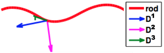
With the Kirchhoff Rod (KR) formulation, a flagellum is described by a 3D space curve for , where is a Lagrangian parameter initialized to be the arclength and is the length of the unstressed rod. Here, we assume the rod length is much greater than the radius and that the rod is isotropic and homogeneous. The associated orthonormal triads follow the right-handed rule. The triad is effectively in the direction of the tangent vector while and are rotations of the normal and binormal vectors, respectively, coinciding with the principal axes of the rod cross section.
Figure 2 shows the centerline of a flagellum discretized as a helix using the centerline approximation with the associated orthonormal triads plotted at one point on the space curve. In the standard KR model, is enforced to be the tangent vector and the rod is inextensible. We employ an unconstrained version whereby an elastic energy penalty is used to numerically maintain the inextensibility of the rod and keep as a unit tangent vector along the rod (Lim et al., 2008; Olson et al., 2013).
The derivation of the internal force and torque in terms of the associated orthonormal triads has previously been described in detail (Lim et al., 2008; Olson et al., 2013). Here, we summarize the main equations of the KR model which are utilized later. The balance of force and torque on a cross section of the rod are
| (5) | |||||
| (6) |
where (units of force per length) and (units of force or torque per length) are part of the external forces applied on the rod. Whereas, and are the internal components of the force transmitted across each section of the rod and are given in terms of and its triads. The components of and can be expanded in the basis of the triads:
| (7) |
for where both and are 3 by 1 vectors at a given along the rod centerline. The constitutive relations for the unconstrained KR are (Olson et al., 2013; Lim et al., 2008)
| (8) |
| (9) |
where the material properties of the rod are characterized through the parameters and for . The bending moduli are , and is the twisting modulus while are the shear moduli, and is the extensional modulus. The strain-twist vector is represented by where is the intrinsic twist and are the geodesic and normal curvatures, respectively, associated with the intrinsic curvature through the equation . This vector determines the preferred configuration of the rod where internal force and torque are generated by differences from the actual and preferred configuration. The preferred strain and twist of the rod can be varied (in time and with respect to arc length parameter ), to propagate planar or helical bending that are representative of sperm flagellar beatforms observed in experiments (Smith et al., 2009b; Woolley & Vernon, 2001).
3 Method of Regularized Brinkmanlets for the Kirchhoff Rod
Given a 3D elastic structure immersed in a Brinkman fluid, the equations of motion include the external forces and torques of the structure on the fluid. The solutions can be calculated exactly in terms of fundamental solutions due to the linearity of the Brinkman equation. However, singular solutions are obtained when evaluating the flow at the location of a point force or torque on the centerline of the structure. Eliminating these singularities requires a regularization method and we utilize the Method of Regularized Brinkmanlets (MRB) (Cortez et al., 2010). The idea is to use a smooth approximation to the singular point force or point torque. The smooth approximation is called a “blob” or regularization function, , and is a radially symmetric function whose width is determined by the regularization parameter . In the limit as , the singular solutions are recovered.
Since we want to capture both the bending and twisting motions of the rod in a 3D infinite fluid, the expression of the force density at a point in the fluid is a contribution of both and , given as
| (10) |
where is the curve corresponding to the centerline of the swimmer and (Olson et al., 2013). In general, we wish to solve the incompressible Brinkman equation in (1)–(2) with body force as in (10) for the local linear velocity and the local angular velocity . Once these are known at , we can update the location of the rod and the associated orthonormal triads using a no-slip condition,
| (11) | |||||
| (12) |
To simplify the derivation, we focus on a single point force and a single point torque , both are constants and applied at the point , given as
| (13) |
where the blob function has units of inverse volume and . We assume that is a radially symmetric function that satisfies the condition in 3D.
3.1 Pressure Calculation
3.2 Linear and Angular Velocity
To find the solution of the linear velocity, we simply substitute (15) back into (1). Given a radially symmetric , one can determine a radially symmetric where for . Using , the linear velocity is given as
| (16) |
On the right hand side of (16), the first two terms correspond to the regularized Brinkmanlet due to a point force . The third and fourth terms are due to a point torque and are the regularized Brinkman rotlet. The angular velocity is then
| (17) | |||||
For convenience in evaluating the solutions of (16) and (17) numerically, we write the local linear and angular velocity as
| (18) | |||||
| (19) | |||||
where and . The coefficient functions are given as:
| , | (20) | ||||
| , | (21) | ||||
| , | (22) |
and additional details on the derivation are given in Appendix A and Section 3.3.
3.3 Regularized Coefficient Functions
Previously, Cortez et al. (2010) detailed two different approaches that can be used to determine appropriate coefficient functions for in the case of 3D Brinkman flow due to regularized point forces (point torques were not considered). The approaches are to either first start with an appropriate blob function or to first start by choosing a regularization of the well known singular solution; each approach leads to a slightly different PDE, resulting in different coefficient functions . On the test cases of flow past a stationary cylinder (2D) or sphere (3D), the error does depend on both the regularization parameter and resistance parameter (Cortez et al., 2010; Leiderman & Olson, 2016). We note that each approach leads to a slightly different regularization of the forces, which in turn, results in a slightly different flow. Carefully chosen blob functions can reduce error and allow for computationally efficient expressions to calculate regularized Stokes and Brinkman flow (Nguyen & Cortez, 2014; Nguyen et al., 2016). On the other hand, a particular regularization of the singular solutions may also lead to desired properties. The best method to use will depend on the application and the desired results in terms of error and computational ease. Hence, we describe how to find the regularized coefficient functions , , and for using both approaches. In Appendix A.3, we compare the blob functions and simulation results for the two approaches. Additionally, in Appendix B.1B.2 we show that when , in both cases, the solution for the linear and angular velocity in (18)–(19) approaches the corresponding regularized solution for Stokes flow (Olson et al., 2013).
3.3.1 Option 1: Regularizing the Fundamental Solutions
The first approach is to solve for the pressure, as well as the linear and angular velocity given in (16)–(17) by regularizing the fundamental solutions (Cortez et al., 2010). That is, the functions and are written as
| (23) |
with such that when , we recover the singular solutions. The corresponding regularized solutions of , and for using (20)–(22) and (23) are detailed in Appendix A.1.
3.3.2 Option 2: Choosing a Blob Function
The second approach, which we use for the results in Section 5, is to first choose a suitable blob function and then derive the corresponding fundamental solutions. We can determine and for a given blob function as:
We utilize the 3D blob function
| (24) |
where the coefficients and are
This blob function was previously derived for a triply periodic Brinkman fluid (Nguyen et al., 2016). The resulting functions and are
4 Numerical Algorithm
The algorithm for calculating the local fluid flow given in (18)–(19), as well as the procedure for updating the configuration of the rod through the no-slip boundary conditions in (11)–(12) is similar to previous derivations (Lim et al., 2008; Lim, 2010; Olson et al., 2013), except that we are now solving the Brinkman equation and have additional terms as described in the previous sections. The centerline of the rod is discretized into immersed boundary points where , for and is a fixed uniform spacing. Let be the time-step index for time where is the time step. Then, is the fluid velocity at time step at rod location .
Assuming a given configuration of the rod (centerline and orthonormal triad) with associated material and intrinsic parameters , , for , the numerical algorithm is as follows:
- 1.
Evaluate the orthonormal triads at half grid points through the use of an orthogonal rotation matrix. Let where is a 3 by 1 vector at time step , so that is the identity matrix and where is the rotation matrix mapping to for . The interpolation to is performed by applying the principal square root of as follows:
(27) Here, is a rotation about the same axis as but by half the angle.
- 2.
Using the updated triad at the half grid point at time step , the internal force and internal moment transmitted across the cross section of the rod is evaluated at using
(28) (29) where is the Kronecker delta. The force and moment vectors are assembled as
(30) The force and torque exerted on the fluid by the rod from (5)–(6) are discretized using a standard central difference to determine and for .
- 3.
The body force in (10) is approximated as
(31) With point forces and torques applied on the fluid, by superposition the linear and angular velocities of the fluid at any point are calculated as
(32) (33) for and .
- 4.
Next, to update the position of the rod, we use the no-slip boundary condition in (11) written in terms of the Euler method as
(34) The orthonormal triads are updated through (12) using
(35) where is an orthogonal matrix rotating around an angle about the axis of the unit vector and is defined as
where is the 3 by 3 identity matrix and is a 3 by 3 antisymmetric matrix. The matrix is often called the Rodrigues rotation matrix (Crisfield, 1997). When determining the new location , higher order methods can be used to update , e.g. second order or fourth order Runge-Kutta methods.
We note that the regularization parameter should be chosen carefully since it is both a numerical parameter and a physical parameter. In the limit as , we approach the singular solution and thus, regularization error will depend on the choice of . In addition, it can be considered a physical parameter since it controls the width of the region where the force is spread. In this KR model, the equations for force and torque balance are derived under the assumption that the rod radius is much smaller than the length of the rod. Thus, we want to ensure that the force is spread to a region of similar radius to that of the rod or filament. Previous studies have also looked at how the error for the method of regularized Brinkmanlets varies as both and vary (Cortez et al., 2010; Leiderman & Olson, 2016). For our application, we choose a fixed regularization parameter for all simulations that matches well with asymptotic results and that lends itself to a range corresponding to the physical radius of the flagellum.
5 Results
We study the effect of varying the resistance parameter on the behavior and overall performance of swimmers propagating planar or helical bending. The time step used is s and the fluid viscosity is set to s-1 (viscosity of water at room temperature). The parameter values and units are summarized in Table 1. In all of our test cases, a force and moment free boundary condition is prescribed, corresponding to
| Parameters | Symbols | Units |
|---|---|---|
| Points along the rod | N | |
| Length | m | |
| Wavelength, Amplitude, Radius | m | |
| Mesh width of the rod | m | |
| Regularization parameter | m | |
| Resistance | m-1 | |
| Time | seconds (s) | |
| Beat Frequency | (1/s) |
5.1 Planar Bending
The Regularized KR method is validated by comparing the numerical and asymptotic swimming speed of a cylindrical tail propagating small amplitude planar bending. In simulations, the KR is initialized as a straight rod with orthonormal triad , , and for a small perturbation to ensure the rod is not initialized in an equilibrium configuration (Lim, 2010). The rod is given the following preferred strain and twist,
which corresponds to a swimmer trying to achieve the preferred configuration of a sinusoidal waveform parameterized by , , and (Olson et al., 2013). Here, the rod is bending in the -plane and the wave propagates along the filament in the direction. The bending amplitude is , is the beat frequency, is the velocity of the propagating wave where is the frequency of the wave, and the wavenumber is where is the wavelength. Since this is a preferred curvature model, the achieved bending amplitude and the swimming speed are emergent properties of the coupled system.
We previously derived the asymptotic swimming speed for a cylinder of infinite-length propagating small amplitude planar bending (Ho et al., 2016). This is calculated as
| (36) |
Here, is the zeroth order modified Bessel function of the second kind, , and where is the radius of the rod. To compare this result to those from the simulations, we set .
(a) (b)


In figure 3(a), we compare the swimming speed results for resistance parameter . The computational swimming speed for the finite-length swimmer is shown with symbols and is determined as the average swimming speed in the -direction along the length of the rod. The asymptotic swimming speed of the infinite-length swimmer is given by in (36) and corresponds to the dashed lines. For different beat frequencies with in the range of 250 to 500, the swimming speeds from the computational method in figure 3(a) scale quadratically with respect to the amplitude (for small amplitude with ), following the trend of the asymptotic swimming speeds. In the simulations, we are assigning a preferred curvature and hence a preferred amplitude of either 0.05, 0.075, 0.1, 0.125, or 0.15. The numerical swimming speeds are plotted in figure 3(a)–(b) with respect to the achieved amplitude (at s); achieved amplitudes are smaller than the preferred amplitudes for this parameter set but the achieved amplitude increases as beat frequency decreases (shown in figure 3(a)) since there is more time for the swimmer to reach the preferred amplitude. We observe excellent agreement between the asymptotic and numerical swimming speeds for a range of , and swimming speeds increase as increases in the case of small preferred amplitude (results not shown).
Since the asymptotic swimming speed in (36) is for an infinite-length swimmer, we explore the emergent swimming speed for different filament lengths in figure 3(b). Here, with , the longest finite-length swimmer at has the best agreement with the asymptotics. Interestingly, the finite-length swimmer achieves slightly faster swimming speeds than the and swimmer for this particular parameter set. We note that since the derivation of the asymptotic swimming speed for the infinite-length swimmer assumed small radius and amplitude, as expected, the asymptotics vary from the numerical simulations for amplitude and the asymptotics fail for a radius . The KR model assumes that the length is much greater than the radius, thus we can simulate rods with this radius when rod length .
| Parameters | SIMS1 | SIMS2 | SIMS3 |
|---|---|---|---|
| Bending modulus, (g m3 s-2) | 3.5 | 0.1 | 1 |
| Twisting modulus, (g m3 s-2) | 3.5 | 0.1 | 1 |
| Shearing modulus, (g m s-2) | 8.0 | 0.06 | 0.6 |
| Stretching modulus, (g m s-2) | 8.0 | 0.06 | 0.6 |
Next, we investigate emergent waveforms and swimming speeds that result from varying the resistance parameter . The swimmers are initialized as straight rods with a preferred planar curvature as in (5.1). The sperm flagellum is represented as a centerline, which we set to (discretized with 301 points). The range of parameters for the preferred waveform are based on previous experiments in different fluid environments where beat frequency ranges from 10–20 Hz, wavelength is in the range of 10–60m, and the mean amplitude can be as large as m (Smith et al., 2009b; Vernon & Woolley, 1999). The stiffness values in the SIMS2 column of Table 2 correspond to experimental values estimated for interdoublet bending resistance and shear resistance in sea urchin sperm (Pelle et al., 2009).
(a)

(b)

Figure 4 shows an example of the velocity field and pressure in the plane around a swimmer propagating planar bending. Due to forces and torques along the length, local vortices of flow are observed, changing direction with the local concavity of the swimmer. Since the swimmer is initialized to be straight, we observe in figure 4(a) at s that there is a sinusoidal wave but it has not yet achieved the preferred amplitude and, in (b), the swimmer achieves the preferred amplitude by s.
(a) (b)


(c) (d)


As the resistance parameter is varied, we observe a non-monotonic change in swimming speed for this same fixed set of parameters. Four different snapshots of the swimmers in time are shown in figure 5 in the plane . At each time point, the five different swimmers correspond to a different simulation at a particular ; they are placed on the same figure for comparison. The same preferred curvature function (with the same amplitude ) is used for each simulation. To monitor the trajectory of the swimmers, the endpoint is also tracked and plotted. At s, shown in figure 5(a), the swimmers immersed in a fluid with smaller resistance parameter (e.g. ) deform and interact with the fluid to start propagating sinusoidal bending while the swimmer in the fluid with remains in a fairly straight line. Figure 5(b) shows that the cases with smaller have swimmers making forward progression. The swimmers in a fluid with resistance parameter , , and 1 are able to achieve an amplitude close to . In contrast, in the case of , the swimmer is not able to reach the desired amplitude and for the simulation, the swimmer is barely moving. This phenomenon occurs because the additional fluid resistance is preventing the swimmers from generating the preferred amplitude. One can imagine that either the fiber radius or the volume fraction of fibers increases as the resistance parameter increases. Thus, the presence of the fibers greatly hinders the ability of the swimmer to generate the preferred waveform.
At time s, figure 5(c) shows that the fastest swimming occurs in the fluid with resistance parameter , where the swimmer’s emergent waveform has a longer wavelength and smaller amplitude than the preferred ones. By time s, shown in figure 5(d), the fastest swimmers are in a fluid with and , the next fastest is , and then . Tracking the last point of each flagellum in figure 5, we observe that each swimmer exhibits a figure-eight motion in the plane of swimming. Greater propulsion in the -direction with each beat of the tail of the swimmer is observed for and 1.
(a) (b)


(c)

To further characterize the emergent behavior of swimmers propagating planar bending, we look at the emergent swimming speed, amplitude , and wavelength for swimmers with different beat frequencies in fluids with different resistance parameter . First, we observe in figure 6(a) that for all of the different beat frequencies, the maximum average swimming speed over the interval 0-1.2 s was obtained when . For , the observed computational swimming speed decreases as decreases. We also observe that the smaller the beat frequency is, the slower the swimmer, in agreement with the asymptotic swimming speed given in (36). When , there is too much resistance in the fluid for the swimmers to achieve the preferred configurations. Figure 6(b) shows that increased beat frequency results in a reduction of the achieved amplitude. In addition, swimmers are able to achieve a larger amplitude when . The emergent wavelength of the swimmers in a Brinkman fluid is also affected by as shown in figure 6(c). Here, the wavelength increases as resistance parameter increases.
In figure 7, a swimmer is shown at s and s. The dashed line corresponds to ; we observe a downward tilt or yaw in the trajectory of the swimmer. The same phenomenon is observed at s regardless of the magnitude of the resistance; however, at higher resistance, the swimmers are not making as much forward progress. In addition, since we are propagating a preferred planar waveform, the average external torque component along the centerline is zero and the swimmer will remain in the plane.


We also investigated the case of doubling the preferred wavelength to while keeping the total length fixed at (representative of both human and sea urchin sperm). The wavelength of human sperm is, in general, less than that of sea urchin sperm, whereas the flagellum of a human sperm is stiffer than that of sea urchin (Lindemann & Lesich, 2010; Smith et al., 2009b; Woolley & Vernon, 2001). With the same stiffness coefficients as in the previous case (SIMS2), we record little to no movement along the rod even in the case of small resistance. We speculate that the the stiffness of the swimmer may play a bigger role at larger wavelengths. To test this, we increase the stiffness coefficients and use the values reported in the SIMS3 column in Table 2, which are more representative of mammalian sperm. Representative results are shown in figure 8. Here, we observe greater forward propulsion with smaller resistance. We also observe the figure-eight motions traced out by the endpoint of the swimmer (not plotted). With the increased stiffness coefficients, trends for the emergent swimming speed, amplitude, and wavelength are similar to those shown in figure 6 as the resistance parameter is varied.
In summary, we have shown that for swimmers propagating planar waveforms, the emergent beatform may be different from the preferred one due to the resistance parameter , as well as the rigidity of the swimmer. For smaller , the swimmer achieves a more obvious sinusoidal configuration and the emergent amplitude gets closer to the preferred one. If the rod is too stiff or if there is too much resistance in the fluid, the rod shows little to no forward motion, and the bending along its length is less likely to occur.
(a) (b)


5.2 Helical Bending
Similar to Section 5.1, we first validate our method for the helical bending case by matching the numerical results to the asymptotic solutions for the case of helical bending with constant amplitude in both bending directions (referred to as spiral bending in Taylor (1952)). The rod is initialized as a right-handed helix parameterized as
| (37) |
and the orthonormal triads are initialized as a rotation of the Frenet frame, given as
Here, the normal vector is N, the binormal vector is B, the tangent vector is T, and the angle of rotation is where is initialized as arc length. The detailed derivation of (37)–(5.2) is in Appendix C. The time-dependent preferred configuration in the form of a helix is given by
where is the constant swimming velocity of the propagating wave and the beat frequency is . The constants and are the intrinsic curvature and torsion, respectively, depending on the radius and the pitch of the helix as follows:
where for wavelength . This preferred curvature corresponds to helical bending propagating along the length of the swimmer, causing the swimmer to progress in the positive -direction. Note that the curvature of the KR is .

| Frequency | Results | |||
|---|---|---|---|---|
| Distance | 0.9006 | 0.8701 | 0.8057 | |
| Radius | 0.5879 | 0.5506 | 0.5334 | |
| Distance | 3.4491 | 3.3135 | 3.0728 | |
| Radius | 0.6327 | 0.5822 | 0.5584 | |
| Distance | 7.9308 | 7.8252 | 7.2561 | |
| Radius | 0.6606 | 0.6010 | 0.5735 |
In this test case, we explore swimming speeds for five different preferred radii () and three different beat frequencies. In simulations, the numerical swimming speed is the average swimming speed in the -direction and is plotted using the achieved radii at s. The computational swimming speeds are compared to the previously derived asymptotic swimming speed for helical bending (Ho et al., 2016), which is twice the swimming speed of the planar bending case given in (36) where we now replace with the radius .
The results are shown in figure 9(a) for , where we observe that the numerical swimming speeds (in marker points) match up well with the asymptotic swimming speeds (in dashed lines), increasing quadratically as the radius (or amplitude) increases. We observe similar swimming speed results when using a resistance parameter in the range of (results not shown). To investigate whether the emergent swimming speed of the helical swimmer is twice as fast as the corresponding planar swimmer (as predicted by the asymptotics), we use the same resistance parameter, beat frequency, and finite-length of the swimmer in the case of planar bending. The results are shown in figure 9(b) and indeed, the helical swimmer is faster than the planar swimmer. We observe that the speed up for finite-length helical vs. planar swimmers varies based on resistance parameter and frequency . In figure 9 for the case of , the helical bending swimmer is 3.1 times faster for and 2.5 times faster for .
We now investigate emergent properties of a rod propagating helical bending as a function of the resistance parameter , using the same initialization as given in (37)–(5.2). In figure 10, the flow field is shown around the swimmer with helical bending. Similar to the swimmer with planar bending (figure 4), we observe local vortices of flow around the swimmer that change with the local concavity of the flagellar centerline. Trajectories for the end point (last point) of the helix propagating helical bending are shown in figures 11–12 and a side view of these helices is shown in figure 13. In all cases, the swimmer traces out a helical trajectory which is consistent with the preferred helical bending. For a smaller beat frequency of in figure 11, the rod does not travel as far as with a higher frequency of in figure 12, as expected based on the asymptotic predictions. The actual distance traveled in 1.2 s is reported in Table 3. In these simulations, the emergent radius of the swimmer is largest in the case of (figure 11(a) and figure 12(a)) and smallest for the case of (figure 11(c) and figure 12(c)). Note that the preferred helix radius is but for this range of stiffness parameters in a Brinkman fluid, the swimmer is only able to achieve a radius in the range of 0.5–0.6.
To illustrate the effect of resistance parameter on helical swimming, we calculate the achieved swimming speeds, radii, and wavelengths for a given preferred beatform for in the range of 0.01–10. The Brinkman swimming speed results for different in figure 14(a) are normalized by the Stokes case (). For small in the range of 0.01–3, we observe that swimming speed is enhanced relative to the Stokes case. On the other hand, when the resistance parameter is larger than 3, the helix swims slower than one in a fluid with no resistance. The maximum value of the swimming speed in this test case is at . In figure 14(b), the emergent radii of the simulated helices are shown; the overall trend is that amplitude or radii decreases as the resistance increases. The emergent wavelength data shown in figure 14(c) fluctuates as the resistance changes. However, the fluctuations in wavelength are within m, which could be due to post-processing to determine the wavelength. Thus, for resistance in the range of 0.01–1, we do not observe a significant change in the wavelength. For larger resistance, we do observe a small decrease in wavelength.
In summary, we have shown that for swimmers propagating helical bending, the emergent beatform may be different from the preferred one due to the resistance term in the Brinkman fluid, which accounts for the presence of a sparse network of fibers. For smaller resistance parameter , the helical configuration has an emergent amplitude that is closer to the preferred one. In comparison to the planar bending case, the helical swimmer is faster for small amplitude, similar to the asymptotic predictions. For all , as the preferred amplitude or radius is increased, the helical swimmer becomes less able to achieve it and thus, swims slower.
(a) (b) (c)


(a) (b) (c)


(a) (b)


(a) (b)


(c)

6 Discussion and Conclusions
We have developed a numerical method to study 3D motility of a swimmer represented as a Kirchhoff rod (KR) that is immersed in a fluid governed by the incompressible Brinkman equations. The linear and angular velocity of the KR are derived using two different approaches, by regularizing fundamental solutions first or by choosing a regularization function and then determining the regularized fundamental solutions. This is an extension of previous work for the case of a KR immersed in a Stokesian fluid (Olson et al., 2013). At each point in time, we utilize the linearity of the Brinkman equation to write the solution as a superposition of fundamental solutions. However, since the forces are a function of the configuration of the KR, the coupled system and emergent swimming speeds are not linear with respect to resistance parameter .
Through the choice of different time-dependent preferred curvature functions, the swimmer propagates planar or helical bending along the length of the rod. The actual force generation and bending of a sperm flagellum is due to the local action of the dyneins (Lindemann & Lesich, 2010), which generate force independently and cause the microtubules to slide relative to one another. The preferred curvature that we utilize is a simplification that is motivated by experimental results of human sperm where the action of the dyneins results in a sinusoidal propagation of curvature (Smith et al., 2009b). In our model, as the resistance parameter is varied, we use the same preferred curvature but local force balance is altered by . Thus, for a given , we observe the emergent flagellar waveform. Our model results are relevant for sperm motility in cases where varying the fluid properties does not change the ability of the dyneins to generate force and propagate a wave of curvature along the flagellum. The parameters for the preferred beat form were taken in the ranges reported for sperm and we vary the resistance parameter in the range of 0 to 10 since it is well known that fiber radii and the volume fraction of the fibers can each vary by several orders of magnitude depending on the time in the menstrual cycle as well as the location in the mammalian reproductive tract (Miki & Clapham, 2013; Smith et al., 2009b).
The stiffness coefficients in the model are chosen from a range of bending and shear moduli reported for sea urchin, rat, and bull sperm (Pelle et al., 2009; Lesich et al., 2008; Schmitz-Lesich & Lindemann, 2004). The KR model is derived from force and torque balance on a cross section, which is simplified to a centerline representation when the rod length is much greater than the radius. Since we want to have a computational centerline that has the appropriate macroscopic moduli, we assign a shear and bending moduli based on experimental values, which is an approach that has been used before in other models of sperm and bacteria (Lim & Peskin, 2004; Olson et al., 2011a). For bending amplitude and wavelength characteristic of human, we observe that swimming speeds are enhanced only when the stiffness of mammalian sperm is used (figure 8), similar to previous computational results (Olson & Leiderman, 2015). When using the lower stiffness values of sea urchin sperm, we observe little to no forward progression (results not shown). We hypothesize that in mammalian sperm, the additional accessory structures called the outer dense fibers (Gaffney et al., 2011), are necessary to make the sperm flagellum stiffer and enhance mammalian sperm progression in fluids with a dense network of proteins.
Although the asymptotic swimming speeds previously derived (Ho et al., 2016) are able to capture the qualitative trends of swimming speed in terms of the dependence on resistance parameter and amplitude, it often overestimates the actual swimming speed for shorter-length filaments and for filaments with larger preferred amplitudes. This is important to consider when using asymptotic swimming speeds to make predictions about the behavior of large amplitude, finite-length swimmers in a fluid with resistance. Our asymptotic analysis predicted that swimmers with helical bending are always two times faster than the corresponding planar swimmer. However, in our experience, this ratio is rarely observed and results are highlighted in Table 4 for . With the current computational method, we observe that helical swimmers with preferred amplitudes , had swimming speeds greater than 2 times that of the corresponding planar swimmer and, in some cases, up to 3.3 times faster (Table 4). In contrast, helical swimmers with larger preferred amplitudes achieve swimming speeds much less than the predicted ratio; in some cases almost 4 times less (results not shown).
| Frequency | Amplitude | Helical Bending | Planar Bending | Ratio |
|---|---|---|---|---|
| Speed | Speed | |||
| 0.075 | 0.6414 | 0.1923 | 3.34 | |
| 0.1 | 1.094 | 0.3399 | 3.21 | |
| 0.125 | 1.6226 | 0.5269 | 3.08 | |
| 0.15 | 2.1963 | 0.7516 | 2.92 | |
| 0.075 | 0.8862 | 0.3002 | 2.95 | |
| 0.1 | 1.5122 | 0.5307 | 2.85 | |
| 0.125 | 2.2443 | 0.8231 | 2.72 | |
| 0.15 | 3.0403 | 1.1747 | 2.59 | |
| 0.075 | 1.1253 | 0.4188 | 2.68 | |
| 0.1 | 1.9214 | 0.7404 | 2.59 | |
| 0.125 | 2.8534 | 1.1487 | 2.48 | |
| 0.15 | 3.8676 | 1.6397 | 2.36 |
In the case of planar and helical bending, we observe an emergent amplitude that generally decreases as the resistance parameter increases, even with the same preferred configuration (figure 6(A) and 14(A)). Due to this decreased amplitude, a decrease in swimming speed for was also observed. This is in contrast to the previously obtained asymptotic results where bending kinematics (amplitude) were prescribed (Ho et al., 2016) and it was possible to obtain higher swimming speeds in fluids with more fibers (larger ). In this previous analysis, it was found that the work required to generate the prescribed amplitude increased greatly as or prescribed amplitude increased. However, in reality, it may not be possible to achieve a swimmer with higher amplitude because microorganisms are not able to generate that much work to maintain the prescribed bending at such high resistance. To further understand the relation between the numerical results presented here and the previous asymptotic analysis, we investigate the asymptotic swimming speeds for a fixed value of work. Equation (36) can be rewritten as
in terms of the nondimensional work , where is detailed in Ho et al. (2016). We fix and consider three different fixed values of as 0.15, 0.2, 0.25. Figure 15(a) shows the relation between the nondimensional swimming speed and the scaled resistance parameter . We observe that for a larger fixed value of work, there is a faster swimming speed. This means that if a swimmer can achieve a higher amount of work, it would be able to swim faster. On the other hand, as the scaled resistance increases, the swimming speed decreases for all three cases with a fixed value of work. This matches our numerical results where swimmers in fluids with large resistance swim slower; this is due to the fact that the forces are based on an energy formulation where emergent beatforms minimize energy in the system (Lim et al., 2008). Hence, work is not able to significantly increase in our 3D Brinkman simulations with the KR, causing amplitude and swimming speed to decrease at high .
(a) (b)

(c)

Experimental studies have shown that emergent waveforms and swimming speeds vary greatly depending on the fluid environment (Smith et al., 2009b; Suarez & Dai, 1992). Since it is both time intensive and costly to perform many experiments tracking sperm motility, the computational framework we present can be used to systematically study 3D flagellar waveforms as protein volume fraction or resistance parameter is varied. In this study, we investigate the emergent waveforms and swimming speeds in the cases of planar and helical bending. We observe non-monotonic swimming speeds with respect to the resistance parameter (figure 6(A) and 14(A)). The enhancement in swimming for a range of may be explained as follows. In the fluid with low resistance (when , this corresponds to no fibers or Stokes flow), the swimmer is able to bend freely (without any effects from the obstacles) and achieve the preferred bending. When the volume fraction of fibers in the fluid is small, the fibers alter or modify the flow in a way that gives an extra push to enhance the swimming velocity. As the resistance parameter increases, the flow decays in a smaller region as described by the screening length, given by . This then results in a different local force and torque balance along the flagellum, with a decrease in the observed amplitude for larger (figure 5).
In order to further characterize this swimming enhancement for small resistance parameter , we will look at an indicator of thrust or propulsive forces since there is not an easy and direct calculation of propulsive forces in a model of force-free swimming with fully coupled and emergent flagellar waveforms. For the planar case, the propulsive forces we report are the body forces of the swimmer from (31) in the direction of swimming. This is calculated as a projection of the forces onto the centerline (line connecting the center of mass and first point or head of swimmer), calculated for each time point. To understand how forces vary in time, in figure 15(b) we look at the integral of the average magnitude of the forces along the length of the flagella over a beat period. For the planar case, recall that the swimmer is initialized as a straight rod and then deforms and interacts with the fluid due to the local force and torque balance to achieve the preferred beat form. As can be seen in figure 5(a)-(b) and 15(b), at 0.0012 and 0.12 s, there is not much of a difference in swimming speeds and magnitude of forces for the different cases of shown. For later times, at 0.6 and 1.2 s, the swimmers have achieved larger amplitude waveforms and the and have progressed further due to the increased force magnitude in the direction of swimming. Since a sperm flagellum can be considered a pusher, the swimming propulsion or thrust will be from the rear or tail end of the swimmer (Pak & Lauga, 2016). To further characterize thrust or propulsive forces, we also calculate the scalar projection of the force onto the centerline at the end of the swimmer as shown in figure 15(c). Here, the forces oscillate in time due to the propagating curvature. Looking at and , we observe the largest thrust in the swimming direction when and the smallest thrust in the case of . There is an upward trend in the propulsive forces, similar to the average over a beat period shown in figure 15(b). We observe similar trends for a range of parameters for both the planar and helical beat form. Another way to understand these emergent swimming speeds and waveforms is to consider the damping stress, the term in (1), which dominates in comparison to the viscous shear stress effects as is further increased (Ingham & Pop, 2005; Kaviany, 2012). Thus, for large (), the shear stress is only generated over a very short distance (Kaviany, 2012), preventing filaments from reaching their preferred configuration and decreasing propulsive forces in the direction of swimming.
We note that this non-monotonic trend in swimming speeds has also been observed for a swimmer propagating planar bending in both 2D and 3D Brinkman fluids (Cortez et al., 2010; Olson & Leiderman, 2015; Leiderman & Olson, 2016). However, in those studies the bending was only allowed in the plane and we know from previous computational analyses that there can be differences in emergent behavior when comparing 2D and 3D models (Olson & Fauci, 2015). Since this non-monotonic behavior has now been observed in a similar range of in both 2D and 3D with different force models, we believe that this is a robust phenomenon. Additionally, since we are fully accounting for the 3D nature of the flagellar beatform in this Kirchhoff rod modeling framework, we believe that the range of corresponding to enhancements in swimming speed, , is more representative of the relevant range. Using this range of , we can back out different possible combinations of fiber volume fraction and fiber radii , and then determine the interfiber spacing using (3)–(4), which are illustrated in figure 1(a) and (b). For example, () could be realized with a fiber radii microns, which would give a volume fraction of 0.021 and an estimated interfiber spacing of microns. Similarly, () could be realized with fiber radii microns, which would give a volume fraction of and an estimated interfiber spacing of microns. We note that for the development of artificial microswimmers, there may be applications where fluids could be created with stationary fibers of radii on the range of 0.3–2 microns, which would give an interfiber spacing of microns. Vaginal fluid fiber radii have been reported as large as 0.35 microns (Rutllant et al., 2005), which would correspond to an interfiber spacing microns. At the larger end of this scale, a human sperm of length 50 microns and wavelength of 10-50 microns (Smith et al., 2009b), would be able to swim freely through the stationary network with little to no interactions with the fibers. If fiber radii were an order of magnitude smaller, this would put interfiber spacing on the order of a micron. The width of the flagellum would fit easily between the fibers but the assumption that the flagellum is not directly interacting with the fibers (either sliding along fibers or hitting fibers) would need to be accounted for if interfiber spacing was actually on the order of a micron. We note that the interfiber spacing in (4) is an estimate whose derivation is based on the assumption of randomly oriented fibers. Recent experimental results have shown that human cervicovaginal mucus actually has pore spacing that is much larger than that predicted by using mucin fiber diameter and volume fraction when assuming randomly oriented fibers (Lai et al., 2009). The larger pore spacing observed was around 18 microns, a range where sperm interactions with the fibers could still be assumed minimal. Thus, additional analysis to determine a better approximation for interfiber spacing for different arrangements of proteins as well as additional experiments to determine a more realistic average fiber spacing of cervical and vaginal fluid are necessary to determine whether the enhancement observed for is in a biologically relevant regime.
Experiments have recorded emergent flagellar waveforms of human sperm in a low viscosity medium consisting of a salt solution with 0.45% serum albumin (very small volume fraction of albumin protein fibers in the fluid) and a high viscosity medium that was obtained by adding 1% methylcellulose (MC) to the low viscosity solution (corresponding to the addition of polymer chains in the fluid) (Smith et al., 2009b). In the Brinkman equation, we are assuming that the fluid viscosity is remaining constant (i.e., the dynamic and effective viscosity are equal) and account directly for the volume fraction of proteins through the resistance parameter (Auriault, 2009). Thus, as a rough approximation, the experiments where viscosity of the gel is increased correlate to our computational results where , and hence volume fraction of proteins or polymers, is increased. In the case of planar and helical swimmers, as shown in figures 6 and 14, we observe a general trend that amplitude decreases as increases. This trend is similar to results of human sperm swimming in MC gels where the higher viscosity gel had a decreased amplitude (Smith et al., 2009b). In contrast, this experimental study showed a significant decrease in the wavelength with the higher viscosity MC gels. In our simulations, we observe an increase in wavelength for the planar swimmer (figure 6) and a very small decrease in wavelength for the helical swimmer (figure 14). In our computational model, as the resistance parameter is varied, this will cause the local force balance to be altered and as a result, we observe the emergent wavelength. The differences in emergent flagellar wavelength between experiments and these computational results could be due to several factors. The higher viscosity MC gels also have a small amount of elasticity (relaxation time of 0.006 s and 0.017 s (Smith et al., 2009b)) and the effective and dynamic viscosity are most likely not equal, which we do not account for in our model.
Sperm cells have been observed to ‘roll’ as they swim (simultaneous rotation of the sperm cell body and flagellum) (Babcock et al., 2014; Smith et al., 2009b). Specifically, human sperm were found to increase rolling from 1.5 Hz to 10 Hz and decrease amplitude as the viscosity of methylcellulose solutions was decreased (Smith et al., 2009b). The tilt or yaw of human sperm was also found to decrease in a gel with higher viscosity (Smith et al., 2009b). Similar to previous computational studies (Olson et al., 2011b; Smith et al., 2009a), we observe the swimmer does not swim exactly straight, but does tilt downward as shown in figure 7. We note that for the planar swimmer, in our computational model, the average external torque component along the centerline is zero and the swimmer will remain in the plane. The angular velocity shows that the KR is rotating, but at a rate much smaller than the experimental data. In addition, simulations with a prescribed beatform swimming in a Brinkman fluid showed an increased angular velocity with increased prescribed amplitude (Ho et al., 2016). However, in our model presented here, we do not observe an increase in angular velocity. With an emergent beatform, the swimmer does not have as much angular velocity since the local force balance allows the swimmer to achieve a different preferred amplitude and does not have to rotate as much to achieve a prescribed amplitude. Our results do differ from experiments in terms of the rolling rate. This could be due to the fact that we are not accounting for the dynamics of a cell body. A computational study of 3D finite-length swimmers with cell bodies and emergent kinematics is necessary to fully understand swimming speed and angular velocity as a function of the resistance. This will be a focus of future studies.
Lastly, the velocity field in this regularized method is given as the superposition of the flow velocity generated by forces exerted on the fluid by a swimmer whose centerline is represented as a KR. As described in Appendix B, as the resistance parameter , we obtain the solution corresponding to that of Stokes equations. We note that the velocity in Eq. (18)–(19) is an approximation to the integral equation using a quadrature rule. Thus, in addition to a regularization error, the evaluation of the integral also introduces a quadrature error (Cortez et al., 2005; Cortez et al., 2010). A recent study of flow past a cylinder (2D) using the method of regularized Brinkmanlets showed the error of the velocity field depends on both the regularization parameter and the resistance (Leiderman & Olson, 2016). In fact, the minimum computed error increased as increased. It would be interesting to further investigate the errors (discretization error and quadrature error) on and off a 3D KR to understand how different blob functions, regularization parameters, and resistance affect the errors.
Acknowledgements
The work of N. Ho was funded, in part, by National Science Foundation grant DMS-1413110. S.D. Olson, was funded, in part, by National Science Foundation grants DMS-1413110 and 1455270. K. Leiderman was funded, in part, by National Science Foundation grant DMS-1413078. The authors thank R. Cortez for helpful discussions.
Appendix A Linear & Angular Velocity
The details for the derivation of the linear and angular velocity are given here and will depend on the choice of the blob function or the regularized functions and where and . Consider the linear velocity in (16) for a constant point force and torque , both applied at where and . The gradient and laplacian terms on the right hand side of (16) can be expanded as
Then, using (20)–(22), the linear velocity can be rewritten as given in (18). Following the same derivation, the angular velocity from (17) can be expanded as
A.1 Option 1: Regularizing the Fundamental Solutions
A.2 Option 2: Choosing a blob function
A.3 Comparing Blob Functions & Methods
The solution to the fluid flow does depend on the particular choice of blob function. The blob function in Eq. (53) has algebraic decay in the range between and as whereas in Eq. (24) decays exponentially, independent of the choice of . To compare these two blob functions fairly, we match their limits and obtain the relation so that they agree at . We plot the functions in Eq. (53) and Eq. (24) for the case when with and . Figure 16 shows the differences for and the agreement in the far-field as the solutions decay to zero. Here, the evaluation at a point force at will give the same value for the flow, but will given slightly different results off of the structure.
The computational swimming speeds for planar bending (using the setup in Section 5.1) is explored using the two different approaches presented in Section 3.3 and detailed in Appendix A.1–A.2. The numerical results are obtained from choosing the blob function (Section 3.3.2) with regularization parameter and regularizing the fundamental solutions (Section 3.3.1) with . In figure 16(b), for the case of , numerical results from both approaches match with the asymptotic swimming speeds. The figure also shows that for this particular case of planar bending, the solutions obtained from the method where a blob function is chosen first yields slightly better agreement in terms of the swimming speeds. In addition, for this method, the achieved amplitude is closer to the preferred amplitude. Thus, computational results that are presented in the results section will be for the case of choosing a particular blob function first (Section 3.3.2).
(a) (b)


Appendix B Linear and Angular Velocity as
The equations of the linear and angular velocity of a KR in a Brinkman fluid are given in (18) and (19), respectively. When , the linear and angular velocity become
In order to show that these equations exactly approach the regularized Stokes flow as , we next need to show that the Brinkman regularized coefficients , , and for approach the Stokes regularized coefficients for a specified blob function. As mentioned in Section 3.3, the coefficients can be calculated in two different ways, which are detailed below.
B.1 Regularizing the Fundamental Solutions
When , the coefficients , and given in (48)–(52) match exactly with those derived in Olson et al. (2013). That is, when , the solution corresponds to the linear and angular velocity of a KR in Stokes flow when using the blob function .
B.2 Selecting a Blob Function
Appendix C Right-Handed Helix Coefficients
We consider the right-handed helix parameterized as
| (86) |
where is the radius of the helix and is the reduced pitch of the helix (the actual pitch is (Goriely & Tabor, 1997)). The task is to write the helix in terms of the arc length and determine the relations among the radius , the pitch , the curvature , and the torsion . The arc length from to is
| (87) |
Then,
| (88) |
where . The helix can be rewritten in terms of arc length as
| (89) |
where the curvature of the helix is determined as
| (90) |
To determine the torsion , we consider the Frenet frame with tangent vector , normal vector , and binormal vector , which satisfy the following (Chouaieb & Maddocks, 2004):
| (91) | |||||
| (92) | |||||
| (93) |
We can also write , , and as
| (94) | |||||
| (95) | |||||
| (96) |
To find the expression for , we need to calculate . From (96) and (91), we have
| (97) | |||||
where . Substituting (94) into (97), we arrive at
| (98) |
Comparing (98) and (93), we have that . The radius and the pitch in terms of the curvature and the torsion are
| (99) |
The right-handed helix can now be written in terms of the curvature and torsion as
Furthermore, if we let be the helix angle between the tangent vector and the -axis, then relates to and as follows,
| (100) |
where is the unit vector in the -direction.
C.1 Material Frame vs. Frenet Frame
Consider an inextensible, unshearable, and uniform rod discretized at the centerline, where is arc length such that for rod length . The corresponding orthonormal triads of the rod are defined such that is perpendicular to and . This director basis relates to the Frenet basis consisting of normal , binormal , and tangent vector as (Djuričković et al., 2013)
| (101) | |||||
where is the rotation angle depending on the arc length . There exists a rotational vector (a strain-twist vector) such that
| (102) |
for
| (103) |
where is the intrinsic curvature, is the geodesic curvature, is the normal curvature, and is the twist (Dineen & Dineen, 1998). Then,
| (104) | |||||
Rewriting the system (101) using Eqs. (94)–(96), and are in terms of and as follows
| (105) |
Taking the first derivative of in (105) and using (104)(105), we have
Comparing with (s) in (93), and or . Then, with (104) we have
or,
Therefore, the strain-twist vector (or the rotating vector) becomes
| (106) |
If the preferred curvature of the helical bending wave has no twisting component, then
| (107) |
Thus, the rotating angle relates to the torsion as
| (108) |
C.2 Helical Bending Wave
References
- Ahmadi et al. (2017) Ahmadi, E., Cortez, R. & Fujioka, H. 2017 Boundary integral formulation for flows containing an interface between two porous media. J. Fluid Mech. 816, 71–93.
- Auriault (2009) Auriault, J. L. 2009 On the domain of validity of Brinkman’s equation. Transp. Porous Media 79, 215–223.
- Babcock et al. (2014) Babcock, D. F., Wandernoth, P. M. & Wennemuth, G. 2014 Episodic rolling and transient attachments create diversity in sperm swimming behavior. BMC Biol. 12 (67).
- Brinkman (1947) Brinkman, H. C. 1947 A calculation of the viscous force exerted by a flowing fluid on a dense swarm of paticles. Appl. Sci. Res. pp. 27–34.
- Chouaieb & Maddocks (2004) Chouaieb, N. & Maddocks, J. H. 2004 Kirchhoff’s problem of helical equilibria of uniform rods. J. Elast. 77 (3), 221–247.
- Cortez (2001) Cortez, R. 2001 The method of regularized Stokeslets. SIAM J. Sci. Comput. 23, 1204–1225.
- Cortez et al. (2010) Cortez, R., Cummins, B., Leiderman, K. & Varela, D. 2010 Computation of three-dimensional Brinkman flows using regularized methods. J. Comput. Phys. 229, 7609–7624.
- Cortez et al. (2005) Cortez, R., Fauci, L. & Medovikov, A. 2005 The method of regularized Stokeslets in three dimensions: Analysis, validation, and application to helical swimming. Phys. Fluids 17, 1204–1224.
- Crisfield (1997) Crisfield, M. A. 1997 Non-Linear Finite Element Analysis of Solids and Structures: Advanced Topics, 1st edn. John Wiley & Sons, Inc., New York, NY, USA.
- Dineen & Dineen (1998) Dineen, S. & Dineen, S. 1998 Multivariate calculus and geometry, 3rd edn. Springer Berlin Heidelberg New York.
- Djuričković et al. (2013) Djuričković, B., Goriely, A. & Maddocks, J. H. 2013 Twist and stretch of helices explained via the Kirchhoff-Love rod model of elastic filaments. Phys. Rev. Lett. 111 (10), 108103.
- Durlofsky & Brady (1987) Durlofsky, L. & Brady, J. F. 1987 Analysis of the Brinkman equation as a model for flow in porous media. Phys. Fluids 30 (11), 3329–3341.
- Elgeti et al. (2010) Elgeti, J., Kaupp, U. B. & Gompper, G. 2010 Hydrodynamics of sperm cells near surfaces. Biophys. J. 99 (4), 1018–1026.
- Fauci & Dillon (2006) Fauci, L. & Dillon, R. 2006 Biofluidmechanics of reproduction. Annu. Rev. Fluid Mech. 38, 371–394.
- Fauci & McDonald (1995) Fauci, L. & McDonald, A. 1995 Sperm motility in the presence of boundaries. Bull. Math. Biol. 57, 679–699.
- Feng et al. (1998) Feng, J., Ganatos, P. & Weinbaum, S. 1998 Motion of a sphere near planar confining boundaries in a Brinkman medium. J. Fluid Mech. 375, 265–296.
- Fu et al. (2010) Fu, H., Shenoy, V. B. & Powers, T. R. 2010 Low Reynolds number swimming in gels. Europhys. Lett. 91.
- Fu et al. (2009) Fu, H., Wolgemuth, C. W. & Powers, T. R. 2009 Swimming speeds of filaments in nonlinearly viscoelastic fluids. Phys. Fluids 21, 033102.
- Gaffney et al. (2011) Gaffney, E. A., Gadêlha, H., Smith, D. J., Blake, J. R. & Kirkman-Brown, J. C. 2011 Mammalian sperm motility: observation and theory. Annu. Rev. Fluid Mech. 43, 501–528.
- Goriely & Tabor (1997) Goriely, A. & Tabor, M. 1997 Nonlinear dynamics of filaments. III. Instabilities of helical rods. P. R. Soc. Lond. A 453, 2583–2601.
- Ho & Suarez (2001) Ho, H. C. & Suarez, S. S. 2001 Hyperactivation of mammalian spermatozoa: function and regulation. Reprod. 122, 519–526.
- Ho et al. (2016) Ho, N., Olson, S. D. & Leiderman, K. 2016 Swimming speeds of filaments in viscous fluids with resistance. Phys. Rev. E 93 (4), 043108.
- Howells (1974) Howells, I. D. 1974 Drag due to the motion of a Newtonian fluid through a sparse random array of small fixed rigid objects. J. Fluid Mech. 64, 449–475.
- Ingham & Pop (2005) Ingham, D. B. & Pop, I. 2005 Transport phenomena in porous media III, 1st edn. Elsevier.
- Katz & Berger (1980) Katz, D. F. & Berger, S. A. 1980 Flagellar propulsion of human sperm in cervical mucus. Biorheol. 17, 169–175.
- Katz et al. (1989) Katz, D. F., Drobnis, E. Z. & Overstreet, J. W. 1989 Factors regulating mammalian sperm migration through the female reproductive tract and oocyte vestments. Gamete Res. 22, 443–469.
- Kaviany (2012) Kaviany, M. 2012 Principles of heat transfer in porous media, 3rd edn. Springer Science & Business Media.
- Lai et al. (2009) Lai, S.K., Wang, Y.Y., Hida, K., Crone, R. & Hanes, J. 2009 Nanoparticles reveal that human cervicovaginal mucus is riddled with pores larger than viruses. Proc. Natl. Acad. Sci. USA 107, 598–603.
- Lauga (2007) Lauga, E. 2007 Propulsion in a viscoelastic fluid. Phys. Fluids 19, 083104.
- Lee et al. (2014) Lee, W., Kim, Y., Olson, S. D. & Lim, S. 2014 Nonlinear dynamics of a rotating elastic rod in a viscous fluid. Phys. Rev. E 90, 033012.
- Leiderman & Olson (2016) Leiderman, K. & Olson, S. D. 2016 Swimming in a two-dimensional Brinkman fluid: Computational modeling and regularized solutions. Phys. Fluids 28 (2), 021902.
- Leshansky (2009) Leshansky, A. M. 2009 Enhanced low-Reynolds-number propulsion in heterogeneous viscous environments. Phys. Rev. E 80, 051911.
- Lesich et al. (2008) Lesich, K., Pelle, D. & Lindemann, C. 2008 Insights into the mechanism of ADP action of flagellar motility derived from studies of bull sperm. Biophys. J. 95, 472–482.
- Lim (2010) Lim, S. 2010 Dynamics of an open elastic rod with intrinsic curvature and twist in a viscous fluid. Phys. Fluids 22, 2066–2083.
- Lim et al. (2008) Lim, S., Ferent, A., Wang, S. X. & Peskin, C. S. 2008 Dynamics of a closed rod with twist and bend in fluid. SIAM J. Sci. Comput. 31, 273–302.
- Lim & Peskin (2004) Lim, S. & Peskin, C. 2004 Simulations of the whirling instability by the immersed boundary method. SIAM J. Sci. Comput. 25 (26), 2066–2083.
- Lindemann & Lesich (2010) Lindemann, C. B. & Lesich, K. A. 2010 Flagellar and ciliary beating: the proven and the possible. J. Cell Sci. 123 (4), 519–528.
- Mattner (1968) Mattner, P. E. 1968 The distribution of spermatozoa and leucocytes in the female genital tract in goats and cattle. J. Reprod. Fertil. 17, 253–261.
- Miki (2007) Miki, K. 2007 Energy metabolism and sperm function. Int. J. Androl. 65, 309–25.
- Miki & Clapham (2013) Miki, K. & Clapham, D.E. 2013 Rheotaxis guides mammalian sperm. Curr. Biol. 23, 443–452.
- Montenegro-Johnson et al. (2012) Montenegro-Johnson, T. D., Smith, A. A., Smith, D. J., Loghin, D. & Blake, J. R. 2012 Modelling the fluid mechanics of cilia and flagella in reproduction and development. Eur. Phys. J. E. 35, 111–118.
- Nguyen & Cortez (2014) Nguyen, HN & Cortez, R 2014 Reduction of the regularization error of the method of regularized Stokeslets for a rigid object immersed in a three-dimensional stokes flow. Commun Comput Phys 15 (1), 126–152.
- Nguyen et al. (2016) Nguyen, H. N., Olson, S. D. & Leiderman, K. 2016 A fast method to compute triply-periodic Brinkman flows. Comput. Fluids 133 (15), 55–67.
- Olson (2014) Olson, S. D. 2014 Motion of filaments with planar and helical bending waves in a viscous fluid. Biological Fluid Dynamics: Modeling, Computation, and Applications, A.M.S. Contemp. Math. Series, Layton A, Olson S (eds). AMS: Providence, RI pp. 109–128.
- Olson & Fauci (2015) Olson, S. D. & Fauci, L. 2015 Hydrodynamic interactions of sheets vs. filaments: attraction, synchronization, and alignment. Phys. Fluids 27, 121901.
- Olson & Leiderman (2015) Olson, S. D. & Leiderman, K. 2015 Effect of fluid resistance on symmetric and asymmetric flagellar waveforms. J. Aero. Aqua. Bio-mech. 4, 12–17.
- Olson et al. (2013) Olson, S. D., Lim, S. & Cortez, R. 2013 Modeling the dynamics of an elastic rod with intrinsic curvature and twist using a regularized Stokes formulation. J. Comput. Phys. 238, 169–187.
- Olson et al. (2011a) Olson, S. D., Suarez, S. S. & Fauci, L. 2011a Coupling biochemistry and hydrodynamics captures hyperactivated sperm motility in a simple flagellar model. J. Theor. Biol. 283, 203–216.
- Olson et al. (2011b) Olson, S. D., Suarez, S. S. & Fauci, L. 2011b Coupling biochemistry and hydrodynamics captures hyperactivated sperm motility in a simple flagellar model. J Theor Biol 283 (1), 203–216.
- Pak & Lauga (2016) Pak, O.S. & Lauga, E. 2016 Theoretical models of low-Reynolds-number locomotion. In Fluid-Structure Interactions in Low-Reynolds-Number Flows (ed. C. Duprat & H. Stone), pp. 100–167. The Royal Society of Chemistry.
- Pelle et al. (2009) Pelle, D. W., Brokaw, C. J., Lesich, K. A. & Lindemann, C. B. 2009 Mechanical properties of the passive sea urchin sperm flagellum. Cell Motil. Cytoskel. 66 (9), 721–735.
- Pozrikidis (1989) Pozrikidis, C. 1989 A singularity method for unsteady linearized flow. Phys. Fluids A 1, 1508–1520.
- Rutllant et al. (2001) Rutllant, J., Lopez-Bejar, M. & Lopez-Gatius, F. 2001 Confocal scanning laser microscopy examination of bovine vaginal fluid at oestrus. Anat. Histol. Embryol. 30, 159–162.
- Rutllant et al. (2005) Rutllant, J., Lopez-Bejar, M. & Lopez-Gatius, F. 2005 Ultrastructural and rheological properties of bovine vaginal fluid and its relation to sperm motility and fertilization: a review. Reprod. Dom. Anim. 40, 79–86.
- Saltzman et al. (1994) Saltzman, W. M., Radomsky, M. L., Whaley, K. J. & Cone, R. A. 1994 Antibody diffusion in human cervical mucus. Biophys. J. 66, 508.
- Schmitz-Lesich & Lindemann (2004) Schmitz-Lesich, KA & Lindemann, CB 2004 Direct measurement of the passive stiffness of rat sperm and implications to the mechanism of the calcium response. Cell Motil Cytoskel 59, 169–179.
- Smith et al. (2009a) Smith, DJ, Gaffney, EA, Blake, JR & Kirkman-Brown, JC 2009a Human sperm accumulation near surfaces: a simulation study. J Fluid Mech. 621, 289–320.
- Smith et al. (2009b) Smith, D. J., Gaffney, E. A., Gadelha, H., Kapur, N. & Kirkman-Brown, J. C. 2009b Bend propagation in the flagella of migrating human sperm, and its modulation by viscosity. Cell Motil. Cytoskel. 66, 220–236.
- Spielman & Goren (1968) Spielman, L. & Goren, S. L. 1968 Model for predicting pressure drop and filtration efficiency in fibrous media. Env. Science Tech. 1 (4), 279–287.
- Suarez (2010) Suarez, S. S. 2010 How do sperm get to the egg? Bioengineering expertise needed! Exp. Mech. 50, 1267–1274.
- Suarez & Dai (1992) Suarez, S. S. & Dai, X. 1992 Hyperactivation enhances mouse sperm capacity for penetrating viscoelastic media. Biol. Reprod. 46, 686–691.
- Suarez & Pacey (2006) Suarez, S. S. & Pacey, A. A. 2006 Sperm transport in the female reproductive tract. Human Reprod. Update 12, 23–37.
- Taylor (1952) Taylor, GI 1952 The action of waving cylindrical tails in propelling microscopic organisms. Proc. Roy. Soc. Lond. Ser. A 211, 225–239.
- Taylor (1951) Taylor, G I 1951 Analysis of the swimming of microscopic organisms. Proc. Roy. Soc. Lond. Ser. A 209, 447–461.
- Teran et al. (2010) Teran, J., Fauci, L. & Shelley, M. 2010 Viscoelastic fluid response can increase the speed of a free swimmer. Phys. Rev. Lett. 104, 038101–4.
- Thomases & Guy (2014) Thomases, B. & Guy, R. D. 2014 Mechanisms of elastic enhancement and hindrance for finite-length undulatory swimmers in viscoelastic fluids. Phys. Rev. Lett. 113, 098102.
- Vernon & Woolley (1999) Vernon, G. G. & Woolley, D. M. 1999 Three-dimensional motion of avian spermatozoa. Cell Motil. Cytoskel. 42 (2), 149–161.
- Woolley & Vernon (2001) Woolley, D. M. & Vernon, G. G. 2001 A study of helical and planar waves on sea urchin sperm flagella, with a theory of how they are generated. J. Exp. Biol. 204, 1333–1345.