Explicit Symplectic Integrator for Particle Tracking in -dependent Static Electric and Magnetic Fields with Curved Reference Trajectory
Abstract
We describe a method for symplectic tracking of charged particles through static electric and magnetic fields. The method can be applied to cases where the fields have a dependence on longitudinal as well as transverse position, and where the reference trajectory may have non-zero curvature. Application of the method requires analytical expressions for the scalar and vector potentials: we show how suitable expressions, in the form of series analogous to multipole expansions, can be constructed from numerical field data, allowing the method to be used in cases where only numerical field data are available.
I Introduction
The magnetic and (in some cases) electric fields used to guide particles in an accelerator are often arranged so that particles ideally follow a curved trajectory. In simple cases, for example a magnetic dipole field, standard expressions can be used to calculate the path of a particle through both the main field and the fringe field regions of the relevant element. However, in more complex cases, calculating particle trajectories can be challenging: such cases include, for example, situations where quadrupole or higher-order multipole fields are included by design within a dipole field, or where account needs to be taken of multipole components occuring from systematic or random errors within the element. In general, the problem of particle tracking can be broken down into two parts. First, an accurate description of the field is needed; and second, the equations of motion through the field must be integrated to find the path followed by a given particle. It is often possible to use a numerical field map to describe the field; then, standard integration algorithms (for example, Runge–Kutta algorithms) can be used to integrate the equations of motion. However, an approach such as this can be computationally expensive, both in terms of the memory needed to store the field data, and in terms of the processing involved in integrating the equations of motion. Furthermore, if there are specific constraints or requirements for the trajectories, then additional challenges can occur. For example, if the tracking must obey the symplectic condition, then an explicit Runge–Kutta integration algorithm cannot be used. Symplectic Runge–Kutta algorithms do exist, but are implicit in the sense that each step requires the solution of a set of algebraic equations that can add significantly to the computation time.
Regarding the description of the field, an alternative approach to a numerical field map is to represent the field as a superposition of a number of “modes”. Given a set of coefficients, the field can be calculated at any position by summing the functions describing the different modes. This is the approach generally taken for multipole fields, for example, where the horizontal and vertical magnetic field components and (respectively) are given by:
| (1) |
The upper limit of the sum, is chosen to provide the accuracy required for the field. The advantages of this approach over a numerical field map are first, that the data describing the field are contained in a relatively small set of coefficients, and second, that the calculation of the field at an arbitrary point does not need interpolation between grid points, which can be an issue in some circumstances for a numerical field map. The field represented by the multipole expansion (1) is independent of the distance along the reference trajectory, and so is appropriate for the main field region within an accelerator element. Depending on the situation being considered, fringe fields may be neglected altogether (as in the “hard edge” approximation), or may be represented using appropriate expressions based, for example, on generalised gradients [1] or formulae representing solutions to Maxwell’s equations with appropriate limiting behaviour [2].
A semi-analytical field description such as (1) has a further advantage over a purely numerical description in the context of particle tracking. In some cases, it is possible to construct explicit transfer maps parameterised, for example, in terms of the mode coefficients and element length: the transfer maps then offer the possibility of greater computational efficiency over numerical integration techniques, such as Runge–Kutta algorithms. Furthermore, if the transfer maps are constructed in an appropriate way, then the tracking can satisfy requirements such as symplecticity. An explicit symplectic integrator for general -dependent static magnetic fields, in systems with a straight reference trajectory, has been presented by Wu, Forest and Robin [3]. Application of the integrator requires the derivatives of the vector potential; it is therefore convenient to have a semi-analytical field description, which allows the derivatives to be expressed in terms of appropriate modes in the same way as the potential itself, thus avoiding the need for taking derivatives numerically.
In elements designed to bend the beam trajectory, it is usually convenient to use a reference trajectory that follows the intended curvature of the path followed by the beam. In such cases, the standard multipole expansion (1) must be modified to give a field that satisfies Maxwell’s equations. For completeness, we would like to have a set of modes that can be used to describe three-dimensional electric and magnetic fields in a co-ordinate system based on a curved reference trajectory, and an efficient method for integrating the equations of motion for particles moving through these fields. In this paper, we present a suitable set of modes for static electric and magnetic fields, and an explicit symplectic integrator for tracking particles through a given field (i.e. a field represented by a certain set of coefficients). The mode decomposition that we use is based on solutions to Laplace’s equation in toroidal co-ordinates; the explicit symplectic integrator is developed following the method of Wu, Forest and Robin [3].
II Definitions
We consider a particle of charge moving (at a relativistic velocity ) through a static electromagnetic field described by a scalar potential and a vector potential . The Hamiltonian for the motion of the particle is [4]:
| (2) |
where a particle with the chosen reference momentum has velocity and relativistic factor , and the scaled vector potential . The independent variable for the system is , corresponding to distance along a reference trajectory. The reference trajectory follows the arc of a circle (in the plane perpendicular to ) with radius . At any point along the reference trajectory, the co-ordinates and describe (respectively) the horizontal and vertical position of the particle in a plane perpendicular to the reference trajectory. The longitudinal co-ordinate is defined:
| (3) |
where the particle arrives at position along the reference trajectory at time (and we can assume that for the reference particle, at time ).
The momenta conjugate to the co-ordinates and are:
| (4) |
where is the relativistic factor of the particle, is the mass, and and are the components of the velocity parallel to the and axes. The longitudinal conjugate momentum is:
| (5) |
where is the total energy of the particle. To simplify some of the formulae, we introduce the “scaled” scalar potential , defined by:
| (6) |
III Derivation of the symplectic integrator
Our method follows the technique of Wu, Forest and Robin [3]. We first extend phase space by introducing a new independent variable , so that is now a dynamical variable with conjugate momentum . The Hamiltonian describing the motion of a particle through an electrostatic field with scaled potential and magnetic field described by a scaled potential is now:
| (7) |
We shall consider the special case where the magnetic field has a uniform vertical field component, which can be represented by a component of the vector potential:
| (8) |
where for a magnetic field of strength . If the field is correctly matched to the curvature of the reference trajectory (so that the reference trajectory is a possible physical trajectory of a particle with momentum ), then . Other components of the magnetic field can be included in the components and of the vector potential.
We assume that the dynamical variables take small values, so that we can approximate the Hamiltonian by expanding the square root to some order in the dynamical variables. In the conventional paraxial approximation, the expansion is made to second order. Here, we expand to third order, and obtain:
| (9) |
where:
| (10) | |||||
| (11) | |||||
| (12) | |||||
| (13) | |||||
| (14) |
Viewed as a Hamiltonian in its own right, the term is integrable, but this is not the case for the other terms, , , or . However, by making appropriate canonical transformations to new variables, we can express , and in integrable form. is of order 3 (or higher) in the dynamical variables; we assume we can drop this term (with some loss of accuracy in the solution to the equations of motion). We can then construct an explicit symplectic integrator as follows:
| (15) |
where:
| (16) |
Continuing the process:
| (17) |
and finally:
| (18) |
The transformations associated with the generator are:
| (19) | |||||
| (20) |
with the transformations of all other variables (not shown explicitly) corresponding to the identity.
Now consider . To find an explicit form for the transformation generated by , we first consider a transformation to new variables, defined by a mixed-variable generating function:
| (21) |
where are the new co-ordinates, are the original momenta, and is defined by:
| (22) |
In Goldstein’s nomenclature [5] is a mixed-variable generating function of the third kind. The new co-ordinates are identical to the original co-ordinates , since:
| (23) |
and similarly for , and . The new momenta are:
| (24) | |||||
| (25) | |||||
| (26) |
and:
| (27) |
In terms of the new variables, can be written:
| (28) |
Viewed as a Hamiltonian, is integrable. The transformations (generated by ) of the dynamical variables are:
| (29) | |||||
| (30) | |||||
| (31) |
Again, the transformations of all other variables (i.e. for those variables not shown explicitly, above) are given by the identity transformation. To apply the transformation , we first transform from the original variables to a set of new variables using (24)–(26); we then apply the transformations (29)–(31), and finally transform back to the original variables using the inverse of the transformations (24)–(26). Note that although the new momenta do not change under the transformation generated by , the change in the co-ordinate leads to a change in , and because the inverse of transformations (24)–(26) have to be calculated at a different point from the original transformations. Thus:
| (32) | |||||
| (33) |
where and correspond to the initial and final values of the co-ordinate under the transformation . There is also a change in ; but this has no effect on the dynamics. In summary, to apply the transformation we need to evaluate (at the initial value of the co-ordinate , and at the final value of the co-ordinate ), and the integral (with respect to ) of the derivative of (with respect to ).
In Section IV.2 we give analytical expressions for the components of the vector potential, based on a three-dimensional “multipole” decomposition of a magnetic field in a region with a curved reference trajectory. It is also possible to write down expressions for the derivatives of the vector potential; however, the integral in (32) needs to be performed numerically. Although this will make a significant contribution to the computational cost for each step in the tracking calculation, in most cases the integral should converge reasonably quickly given that the derivative of the potential (which is related to the field strength) should vary slowly over the range of the integral (corresponding to the change in the co-ordinate over the tracking step).
The transformation with generator may be handled in a similar way to that generated by , by first transforming to new variables. For the case of , we use the mixed-variable generating function:
| (34) |
where:
| (35) |
Note that the new variables in this case (co-ordinates , , and , and momenta , , and ) are formally different from the variables in the previous case; but to avoid introducing further notation, we use the same symbols. The transformations (generated by ) of the dynamical variables are:
| (36) | |||||
| (37) | |||||
| (38) | |||||
| (39) |
where:
| (40) |
and and are the values of before and after the transformation, respectively. The variables and are unchanged by the transformation.
Finally, we find explicit expressions for the transformation with generator by again first transforming to new variables. In this case, we use a mixed-variable generating function:
| (41) |
where are the new co-ordinates, and are the original momenta. The new co-ordinates are identical to the original co-ordinates, since:
| (42) |
and similarly for , and . The new momenta are:
| (43) | |||||
| (44) | |||||
| (45) |
and:
| (46) |
In terms of the new variables, can be written:
| (47) |
which is an integrable Hamiltonian, leading to the transformations:
| (49) | |||||
| (50) | |||||
| (51) | |||||
Again, transformations of the variables not given explicitly above, are equal to the identity.
IV -dependent fields in toroidal co-ordinates
Applying the symplectic integrator described in Section III involves derivatives of the scalar potential, and derivatives and integrals of the vector potential. It is therefore helpful to have analytic representations of the scalar and vector potentials, from which expressions for the derivatives and integrals may be found. In practice, however, only a purely numerical representation of the potentials may be available (giving, for example, the values of the potentials on a grid of discrete points over some region of space). With a straight reference trajectory (), it is possible to fit the coefficients of series representations of the potentials, for example using generalised gradients [1]; the series representation gives the functional dependence of the potential on the co-ordinates, and this therefore provides a suitable representation for applying the integrator.
A similar approach is possible in the case that the reference trajectory has some non-zero curvature. Expressions for “curvilinear multipoles” (multipole fields around curved reference trajectories) have been given by McMillan and others [7, 8, 9, 10], and have been implemented in the tracking code Bmad [11]. However, the available expressions are not ideal for use where the potential is given in purely numerical form. In much of the previous work, the multipoles are expressed in terms of the transverse Cartesian co-ordinates, and : obtaining the multipole coefficients then involves fitting polynomials to the numerical data along either the or axis [12]. The nature of the potential (which satisfies Laplace’s equation) is such that residuals to the fit will grow exponentially with distance from the line along which the fit is performed. A more robust approach is based on fitting to a surface bounding some region of space enclosing the reference trajectory: within the surface, the residuals decrease exponentially with distance from the surface. Although the residuals will still grow exponentially outside the region enclosed by the surface, if the surface is chosen appropriately then the enclosed region will cover the volume of interest for particle tracking.
To obtain a multipole decomposition based on fitting numerical data on a surface, it is convenient in the case of a curved reference trajectory to work in toroidal co-ordinates [13, 14]. The co-ordinates in the transverse plane are illustrated in Fig. 1. The toroidal co-ordinates and are related to the accelerator co-ordinates and (Cartesian co-ordinates in a plane perpendicular to the reference trajectory) by:
| (52) | |||||
| (53) |
where is the radius of curvature of the reference trajectory. The longitudinal co-ordinate (the distance along the reference trajectory) is related to the toroidal co-ordinate by:
| (54) |
A surface enclosing the reference trajectory can be defined by specifying a fixed value for the co-ordinate : a surface defined by for and resembles a torus. If numerical field data are available for the scalar and vector potentials on such a surface, then it is possible to fit the coefficients of series expansions for the scalar and vector potentials (up to some desired order) to the data. This produces expressions that are suitable for use in the explicit symplectic integrator described in Section III. We first discuss the case of the scalar potential, and then extend the results to the vector potential.
IV.1 Scalar potential in toroidal co-ordinates
In terms of the toroidal co-ordinates, an harmonic potential (such that ) may be written [13, 15]:
| (55) |
where the are coefficients representing the strength of a multipole component . The multipole components are given by:
| (56) |
where is an associated Legendre polynomial of the first kind, and:
| (57) |
An algorithm for computation of the associated Legendre polynomials with positive has been presented by Segura and Gil [16]; values for negative are readily obtained using [17]:
| (58) | |||||
where is an associated Legendre polynomial of the second kind. Note that for integer (which is the case of interest here), the term in in (58) vanishes.
We shall show in Section IV.3 that each component has properties that may be expected of a multipole of order , with corresponding to a dipole, a quadrupole, and so on. Note that a normal dipole deflects a particle horizontally, whereas a skew dipole deflects a particle vertically.
Given numerical data for a potential , the coefficients may be obtained from:
| (59) |
where is a fixed value of that defines the surface (enclosing the reference trajctory, ) on which the fit to the numerical data is performed, and is a normalising factor:
| (60) |
As an alternative to calculating the coefficients from the scalar potential, they may be calculated from the electric field components. The electric field is derived from the potential by:
| (61) |
The component of the field (tangential to a line defined by fixed values of and ) is given by:
| (62) |
The coefficients can then be found from the values of on a surface :
| (63) |
where:
| (64) |

To apply the symplectic integrator described in Section III, we need the derivatives of the potential with respect to the Cartesian co-ordinates. The derivates can be obtained from:
| (65) | |||||
| (66) |
and:
| (67) |
For a given multipole component (56) the derivatives with respect to the toroidal co-ordinates and are:
| (68) | |||||
and:
| (69) | |||||
Finally, we need the derivatives of the toroidal co-ordinates with respect to the Cartesian co-ordinates . The toroidal co-ordinates can be expressed in terms of the Cartesian co-ordinates as follows:
| (70) |
We then find:
| (71) | |||||
and:
| (72) | |||||
The derivatives of the potential with respect to the Cartesian co-ordinates can be found by using equations (68), (69), (71) and (72) in equations (65) and (66). Tracking a particle through a field described by a scalar potential can then be achieved by using the potential and its derivatives (with respect to and ) in the symplectic integrator described in Section III.
IV.2 Vector potential in toroidal co-ordinates
To apply the explicit symplectic integrator to a particle moving through a magnetic field, we need expressions for the components of the vector potential. Since we address the case of a curved reference trajectory, we assume that the magnetic field has a (normal) dipole component derived from the longitudinal component of the vector potential (8). Other components of the magnetic field (corresponding to quadrupole, or higher-order multipole components) may be derived from the transverse components of the vector potential. In toroidal co-ordinates, these components may be expressed as follows:
| (73) | |||||
| (74) |
where the functions are given by (56). In the case that (i.e. the longitudinal component of the vector potential is zero, so that in (8)), and for all , , it is found that:
| (75) |
with given by (55). Hence, the magnetic field derived from the vector potential with components (in toroidal co-ordinates) given by (73) and (74) has the same form as the electric field derived from the scalar potential given by (55).
To apply the symplectic integrator described in Section III, we require the components of the vector potential in Cartesian co-ordinates, and their derivatives. Given the components in toroidal co-ordinates, the components in Cartesian co-ordinates are obtained from:
| (76) | |||||
| (77) |
where the normalising factor is:
| (78) | |||||
The derivatives of and with respect to the Cartesian co-ordinates and can be expressed in terms of the derivatives with respect to the toroidal co-ordinates and :
| (79) | |||||
| (80) |
Given (73) and (74), the derivatives of and with respect to the toroidal co-ordinates may be found from the second derivatives of the scalar potential:
| (81) | |||||
| (83) |
where:
| (84) | |||||
| (85) | |||||
| (86) | |||||
| (87) | |||||
| (88) |
IV.3 Examples of multipole potentials in toroidal co-ordinates
To illustrate the scalar potential given by (55), we consider the case that the potential is independent of the longitudinal co-ordinate, : as a consequence, we need to include only a single longitudinal mode, in the summation in (55). With a straight reference trajectory (), we expect a multipole potential to take the form:
| (89) |
where the real and imaginary parts of the coefficient determine the strengths of the normal and skew components of the field. Hence, in a normal multipole field of order the potential varies along the axis as:
| (90) |
and along the axis as:
| (91) |
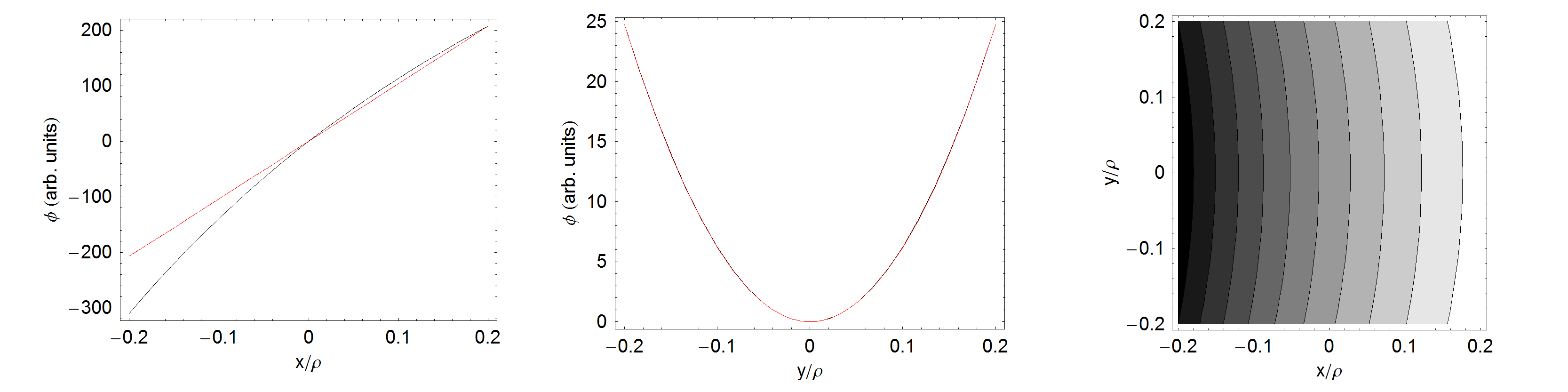
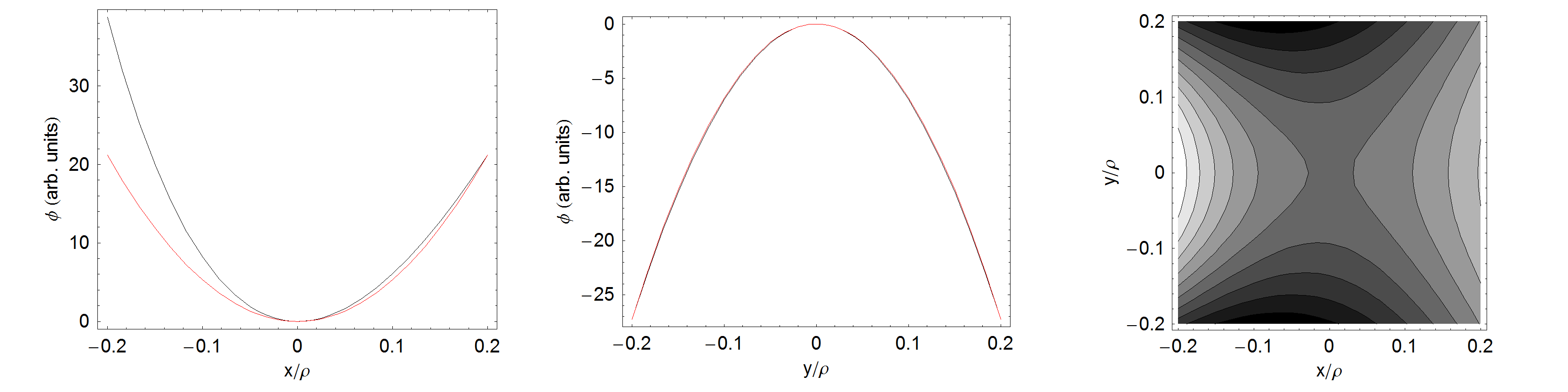
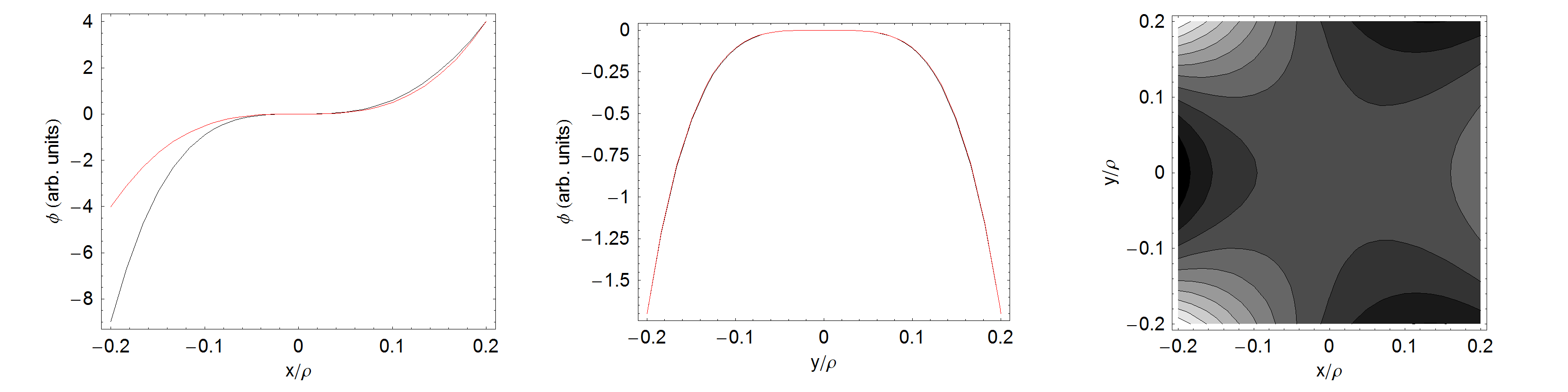


With a curved reference trajectory, we expect to see similar behaviour in the dependence of the potential for a given order of multipole on the and co-ordinates, but with some difference from the dependence given in (89) arising from the curvature. One way to show a similarity between multipoles with straight and curved reference trajectories would be to expand the potential in the case of a multipole with curved reference trajectory as a series in and ; unfortunately, the fact that the limit , corresponds to makes it problematic to obtain the appropriate series. However, we can plot the potential for a given order of (normal or skew) multipole as a function of and : plots for dipoles, quadrupoles and sextupoles are shown in Fig. 2 (normal multipoles) and Fig. 3 (skew multipoles).
From Fig. 2 (top), for example, we see that for a normal dipole the potential has an approximately linear dependence on . With a straight reference trajectory, we would expect the potential to be independent of ; however, the curvature of the reference trajectory introduces a second-order dependence of the potential on . In the case of a normal quadrupole (Fig. 2, middle), the potential has a (roughly) quadratic dependence on both and : this again corresponds to the behaviour that we would expect in the case of a straight reference trajectory. Because the curvature of the reference trajectory breaks the symmetry between positive and negative values of , the effect of the curvature is more evident in the dependence of the potential on , than in the dependence of the potential on . For a skew quadrupole (Fig. 3, middle), the potential with a straight reference trajectory is exactly zero along the and axes. With a curved reference trajectory, the potential is zero along the axis (as required by symmetry); but there is a relatively weak fourth-order dependence of the potential on (with ). Other cases demonstrate the general behaviour we would expect for a multipole potential in a straight co-ordinate system, but with some differences arising from the curvature of the reference trajectory.
V Test cases
To illustrate application of the explicit symplectic integrator presented in Section III, we consider three test cases: a curvilinear magnetic skew sextupole, a curvilinear electrostatic quadrupole, and the fringe field region of an electrostatic quadrupole in the g-2 storage ring [18, 19, 20, 21]. The first two cases are “artificial” in the sense that they are based on fields described by a small number of components; the third case is more realistic, and uses field component coefficients fitted to numerical data obtained from a modelling code. In each case, we track a particle with some chosen initial conditions through the field using the explicit symplectic integrator. For comparison, we also integrate numerically the (Hamiltonian) equations of motion derived from the exact Hamiltonian (2). All calculations are performed in Mathematica 5.0 [6]; for numerical integration of the equations of motion derived from the Hamiltonian (2), we use the NDSolve function with default settings; although this provides a non-symplectic integration, it should achieve good accuracy.


V.1 Curvilinear magnetic skew sextupole
As a first illustration of the explicit symplectic integrator presented in Section III we consider the motion of a particle in an electric field with (scaled) magnetic scalar potential given by:
| (92) | |||||
The field derived from this potential has the characteristics of a skew sextupole field, as shown in Fig. 4. We choose the field strength such that , and use a radius of curvature for the reference trajectory m. A dipole magnetic field is included, represented by the longitudinal component of the vector potential (8), but with so that there is a slight mismatch between the field and the curvature of the reference trajectory.
For the reference particle, we choose , and the initial conditions for the particle to be tracked are:
We track the particle using the explicit symplectic integrator presented in Section III, from to , with a step size of . The integration required in (32) is approximated by Simpson’s rule:
where the derivative is evaluated in each case at the appropriate (fixed) values of and , and at the indicated value of . A similar approximation is made for the integration in (38). Although these approximations will lead to some symplectic error, this should be small for small step size. In cases where symplecticity is important, more accurate integration routines can be used, though at greater computational cost.
The tracking results are shown in Fig. 5. There is good agreement between the two integration methods.

V.2 Curvilinear electrostatic quadrupole
As a second illustration of the explicit symplectic integrator presented in Section III we consider the motion of a particle in an electric field with (scaled) scalar potential given by:
| (95) | |||||
This represents the potential for a “curvilinear” electrostatic quadrupole, with a strength that varies with longitudinal position along the reference trajectory. The transverse and longitudinal variation of the field are described by and (respectively) in Eq. (55). The potential is illustrated in Fig. 6. We choose the field strength , and use a radius of curvature for the reference trajectory m. We include a magnetic field, represented by the vector potential (8), but we introduce a small mistmatch between the field and the curvature of the reference trajectory by setting .


For the reference particle, we choose , and the initial conditions for the particle to be tracked are:
| (96) |
We track the particle using the explicit symplectic integrator presented in Section III, from to , with a step size of . For comparison, we also integrate numerically the (Hamiltonian) equations of motion derived from the exact Hamiltonian (2). The tracking results are shown in Fig. 7, and again we see good agreement between the two integration methods.

V.3 g-2 storage ring electrostatic quadrupole
As a final example of application of the symplectic integrator, we consider the fringe field regions of the electrostatic quadrupoles in the g-2 storage ring [18, 19, 20, 21]. Values for the potential were calculated (using an FEA code) at points on a uniform Cartesian grid; the values of the potential on a surface defined (in toroidal co-ordinates) by were then obtained by (spline) interpolation. On the surface , we used 120 grid points in , with , and 80 grid points in , with (such that the ends of the quadrupole electrodes are at approximately ). The reference radius for the co-ordinate system is taken to be the radius of curvature of the reference trajectory in the g-2 storage ring, m: this is the radius of the closed orbit for muons with momentum 3.094 GeV/c. The value of then corresponds, for , to a point with m and , in the conventional accelerator co-ordinate system, with the origin for the and co-ordinates on the reference trajectory.
Based on equation (55), coefficients were calculated so that the potential on any grid point can be found from:
where , with (so that corresponds to a sine function with quarter period equal to , i.e. the range of over which values for the potential are given). The values of are obtained essentially by a discrete Fourier transform of the potential on the given grid points. Mode numbers and are used. The truncation in the azimuthal mode number (compared to the number of data points available) means that the data are not fitted perfectly; however, the contribution of modes (multipoles) of order is found to be small. Note that the dominant multipole is the quadrupole component, .
The potential as a function of (at and ) is shown in Fig. 8, and as a function of (at and at , with in both cases) in Fig. 9. In the lower plot in Fig. 9, we see that the variation of the potential with the “azimuthal” co-ordinate in the fringe-field region (about 30 mm from the ends of the electrodes) is significantly distorted from a simple sine wave, indicating the presence of higher-order multipoles.


Using the coefficients we can calculate the potential at any point within the surface on which the fit is performed. As an example, Fig. 10 shows the potential as a function of (for ) and as a function of (for ). In each plot, the black line shows the potential at and the red line shows the potential at : the larger value of corresponds to a value of that is a factor of smaller than the value of at , so that the potential (for a pure quadrupole) is expected to be smaller by a factor of two. The expected behaviour of the potential (as a function of ) is indeed what we observe.


Tracking a particle through the fringe field of an electrostatic quadrupole using the symplectic integrator described in Section III requires the derivatives of the potential with respect to the accelerator co-ordinates, , and . The derivatives can be calculated (at any point within the surface used to fit the coefficients for the given potential) using equation (), together with (71) and (72). Some example results from tracking a muon through the fringe field are shown in Fig. 11. The black points in Fig. 11 show the muon trajectory calculated using the symplectic integrator for the detailed fringe-field model, i.e. the model based on the numerical data for the scalar potential. The red line shows the results of an integration using a (non-symplectic) adaptive Runge–Kutta integration of the equations of motion in the same field. The blue line shows the results of a Runge–Kutta integration of the equations of motion through a region with the same magnetic field, but with a “hard-edge” model for the electric field. The hard-edge model is constructed so that the scalar potential is zero up to a point , and is given simply by for . The value of is chosen to correspond to the focusing potential in the body of the quadrupole found from the numerical data for the scalar potential. The point is chosen so that the integrated gradient, in the hard-edge model is equal to the integrated gradient in the fringe-field model.

There is good agreement between the symplectic integrator and the Runge–Kutta integrator for the detailed fringe-field model. There is little difference between the detailed fringe-field model and the hard-edge model for the horizontal motion, which is dominated by the magnetic field (that is the same in both cases). There is some small but observable difference between the detailed fringe-field model and the hard-edge model for the vertical motion. The change in the vertical momentum after integrating through the full region is approximately the same in both cases: this is expected, since the length of the quadrupole field in the hard-edge model was chosen to give the same integrated focusing strength as the detailed fringe-field model. However, the fact that the change in the vertical momentum occurs at a discrete point in the hard-edge model leads to a slightly larger difference between the models in the vertical co-ordinate at the end of the integration. It is unclear what impact this may have on the beam dynamics in the storage ring, but it is possible that it may lead to an observable effect over a sufficiently large number of turns.
Acknowledgements.
We wish to thank Bruno Muratori for useful discussions, and members of the g-2 Collaboration for help and support with studies of the g-2 electrostatic quadrupoles. In particular, we are grateful to Wanwei Wu for providing field data.References
- [1] M. Venturini and A.J. Dragt, “Accurate computation of transfer maps from magnetic field data”, Nuclear Instruments and Methods in Physics Research Section A (1999), pp. 387–392.
- [2] B. Muratori, J.K. Jones and A. Wolski, “Analytical expressions for fringe fields in multipole magnets”, Physical Review Accelerators and Beams (2015).
- [3] Y.K. Wu, E. Forest and D.S. Robin, “Explicit symplectic integrator for -dependent static magnetic field”, Physical Review E (2003).
- [4] A. Wolski, “Beam dynamics in high energy particle accelerators”, Imperial College Press (2014).
- [5] H. Goldstein, C.P. Poole Jr. and J.L. Safko, “Classical Mechanics”, Addison–Wesley (3rd edition, 2001).
- [6]
Wolfram Mathematica,
https://www.wolfram.com/mathematica/ (accessed 12 April 2018). - [7] E.M. McMillan, “Multipoles in cylindrical coordinates”, Nuclear Instruments and Methods 127 (1975), pp. 471–474.
- [8] T. Zolkin, “Sector magnets or transverse electromagnetic fields in cylindrical coordinates”, Physical Review Accelerators and Beams (2017).
- [9] P. Schnizer, E. Fischer and B. Schnizer, “Cylindrical circular and elliptical, toroidal circular and elliptical multipoles fields, potentials and their measurement for accelerator magnets,” arXiv:1410.8090 [physics.acc-ph] (29 October, 2014).
- [10] L. Brouwer, S. Caspi, D. Robin, W. Wan, “3D toroidal field multipoles for curved accelerator magnets”, Proceedings of IPAC2013, Pasadena, CA, USA (2013), pp. 907–909.
- [11] D. Sagan, “The Bmad Reference Manual”, section 14.3, https://www.classe.cornell.edu/ dcs/bmad/manual.html (revision 28.24, 11 June 2017), pp. 252–254.
- [12] A.T. Herrod, S. Jones, A. Wolski, I.R. Bailey, M. Korostelev, “Modelling of curvilinear electrostatic multipoles in the Fermilab muon g-2 storage ring”, Proceedings of IPAC2017, Copenhagen, Denmark (2017), pp. 3837–3839.
- [13] G. Arfken, “Toroidal coordinates ”, Mathematical Methods for Physicists, section 2.13, Academic Press (2nd edition, 1970), pp. 112–115.
- [14]
E.W. Weissten,
“Toroidal coordinates”,
MathWorld – A Wolfram Web Resource,
http://mathworld.wolfram.com/
ToroidalCoordinates.html (12 June, 2017). - [15]
E.W. Weissten,
“Laplace’s equation – toroidal coordinates”,
MathWorld – A Wolfram Web Resource,
http://mathworld.wolfram.com/
LaplacesEquationToroidalCoordinates.html (12 June, 2017). - [16] J. Segura and A. Gil, “Evaluation of toroidal harmonics”, Computer Physics Communications 124 (2000), pp. 104-122.
- [17] M. Abramowitz and I. Stegun (editors), “Handbook of Mathematical Functions with Formulas, Graphs and Mathematical Tables”, Martino Fine Books (2014).
- [18] Muon g-2 Collaboration, “Muon g-2 Technical Design Report”, Fermilab-FN-0992-E, arXiv:1501.06858 (January 2015).
- [19] Muon g-2 Collaboration, “Muon g-2 Technical Design Report, Chapter 13: The electrostatic quadrupoles (ESQ) and beam collimators”, Fermilab-FN-0992-E, arXiv:1501.06858 (January 2015), pp. 395–422.
- [20] W. Wu and B. Quinn, “Beam dynamics in g-2 storage ring”, Proceedings of IPAC2017, Copenhagen, Denmark (2017), pp. 817–819.
- [21] Y.K. Semertzidis, G. Bennett, E. Efstathiadis, F. Krienen, R. Larsen, Y.Y. Lee, W.M. Morse, Y. Orlov, C.S. Ozben, B.L. Roberts, L.P. Snydstrup, D.S. Warburton, “The Brookhaven muon (g-2) storage ring high voltage quadrupoles”, Nuclear Instruments and Methods in Physics Research Section A (2003), pp. 458–484.