Equivalence between spectral properties of graphs with and without loops

Eleonora Andreotti^* Daniel Remondini Armando Bazzani

Abstract

In this paper we introduce a spectra preserving relation between graphs with loops and graphs without loops. This relation is achieved in two steps. First, by generalizing spectra results got on $(m,k)$ -stars to a wider class of graphs, the $(m,k,s)$ -stars with or without loops. Second, by defining a covering space of graphs with loops that allows to remove the presence of loops by increasing the graph dimension. The equivalence of the two class of graphs allows to study graph with loops as simple graph without loosing information.

Eleonora Andreotti^∗

Department of Physics, University of Torino, 10125 Torino, Italy

Daniel Remondini and Armando Bazzani

Department of Physics and Astronomy (DIFA), University of Bologna, 40127 Bologna, Italy

INFN Section of Bologna, Italy

1 Introduction

In graph theory there are many areas of social networks and biological networks in which multigraphs (i.e. graphs comprising loops and multiedges) arise more naturally than simple graphs [WF94, PW99, Rob13]. Moreover, these multigraph structures also emerge when several types of graph homomorphisms are applied, such as aggregation, scaling and blocking procedures, [Sha15, Sco00, Ray14].
Many extensively used approaches in network analysis only consider simple graphs: only single edges between two different vertices are allowed, and self relations (loops [Big93, GR01, Chu97]) are excluded. Moreover, with respect to the graph Laplacian operator, we can consider the case of ”generalized graph Laplacians” [BLS07] in which the diagonal terms (corresponding to topological or weighted loops) can be considered as the ”potential” of an Hamiltonian operator, useful for example when studying protein structure by network-based approaches starting from their Contact Maps [PRP+13, MFR16]. In practice, simple graphs are often derived from multigraphs by collapsing multiple edges into a single one and removing the loops [Ray14, Bon76]. This procedure is applied since many algorithms and theorems work only for simple graphs, but these approaches may discard inherent information in the original network.

In this manuscript, we propose a suitable method to treat graphs with loops as simple graphs, keeping the same eigenvalue spectrum and as much as possible the eigenvectors of their adjacency and transition matrices. One of the results of the paper is the possibility to associate a Laplacian matrix to a graph with loops that allows to study its topological properties.
Because eigenvalues and eigenvectors describe completely the matrix, by preserving the adjacency (or transition) matrix spectra (eigenvalues and eigenvectors) we maintain the informations and properties of the graphs as much as possible. In this way, graphs with loops can be studied with tools extensively used for simple graphs.
To define the correspondence between graphs and simple graphs, we introduce an extension of the structure and the results discussed in [ARSB18]; then we build a correspondence between two classes of subgraphs, namely the $(m,k,s)-$ star with loops and the $(m,k,s)-$ star without loops.
The paper is organized as follows: after some preliminary remarks (section 2), in section 3 we generalize the class of $(m,k)$ -star in graphs to a wider class of graph, the $(m,k,s)$ -star with or without loop, in order to extend the results obtained in [ARSB18]. Then, we show a connection between eigenvectors and eigenvalues of graphs with and without loops. In particular, each vertex with loops can be described as an $(1,k,-)$ -star with loop: we will give a useful tool to replace the looped vertices with an $(2,k,s)$ -star without loop by maintaining the same spectrum.
Thanks to these results it is possible to describe a graph with loop by a graph without loop and to define the Laplacian matrix of the correspondence graph. Finally, in section 4 we draw some conclusions and discuss an outlook on future developments.

2 Preliminary definitions

We consider an undirected weighted connected graph $\mathcal{G}:=(\mathcal{V},\mathcal{E},w)$ , where the edges $\mathcal{E}$ connect $n$ vertexes $\mathcal{V}$ and $w$ is the edge weight function: $w:\mathcal{E}\rightarrow\mathbb{R}^{+}.$ Let $A$ be the weighted adjacency matrix, which is symmetric since the graph is undirected ( $A\in Sym_{n}(\mathbb{R}^{+})$ ),

A_{ij}=\begin{cases}w(i,j),&\mbox{if $i$ is connected to $j$ }(i\sim j)\\ 0&\mbox{otherwise }\end{cases}

where $i,j\in\mathcal{V}$ .
Since the graph is not necessarily simple, any diagonal element of $A$ could be nonzero.
If the graph $\mathcal{G}$ is simple, we introduce the strength diagonal matrix $D$ :

D_{ij}=\begin{cases}\sum_{k=1}^{n}w(i,k),&\mbox{if }i=j\\ 0&\mbox{otherwise }\end{cases}

and we define the Laplacian matrix $L\in Sym_{n}(\mathbb{R})$ and normalized Laplacian matrix $\mathcal{L}\in Sym_{n}(\mathbb{R})$ as

L:=D-A,\quad\mathcal{L}:=D^{-1/2}(D-A)D^{-1/2}.

Whenever we refer to the $k$ -th eigenvalue of a Laplacian matrix, we will refer to the $k$ -th nonzero eigenvalue according to an increasing order.

Furthermore, we observe that by defining the transition matrix $T$ as $T:=D^{-1}A$ ( $T$ defines the transition probabilities of a random walk on the graph) , the eigenvalue spectrum $\sigma(T)$ is related to $\sigma(\mathcal{L})$ . Indeed $T$ is similar to $\tilde{A}:=D^{-1/2}AD^{-1/2}$ via the invertible matrix $D^{1/2}$ and and it is easy to prove that the following statements are equivalent

S.1

$v$ is an eigenvector of $\tilde{A}$ with eigenvalue $\lambda$
S.2

$v^{T}D^{1/2}$ is a left eigenvector of $T$ with the eigenvalue $\lambda$
S.3

$D^{-1/2}v$ is a right eigenvector of $T$ with eigenvalue $\lambda$

Then we consider the relation between $\sigma(\tilde{A})$ and the spectrum $\sigma(\mathcal{L})$ using the equivalence of the following statements

S.1

$v$ is an eigenvector of $\tilde{A}$ with eigenvalue $\lambda$
S.4

$v$ is an eigenvector of $\mathcal{L}$ with the eigenvalue $1-\lambda.$

This relation will be very useful later in order to link the Laplacian of graphs with and without loops.

For the classical results on Laplacian matrices and their application to network theory, one may refer to [Chu97, CH10, New10, AM85, Mer94].

3 Definition of $(m,k,s)$ -star with and without loop

In the present section, we define a wider class of weighted $(m,k)$ -stars (we refer to it as the weighted $(m,k,s)$ -stars), to generalize the results obtained on multiple eigenvalues of Laplacian matrices, transition and adjacency matrices[ARSB18]. Then we consider the problem of introducing a correspondence between the class of weighted $(m,k,s)$ -stars and the class of weighted $(m,k,s)$ -stars with loops. In this way it is possible to remove loops from a weighted $(m,k,s)$ -stars with loops in graph by replacing it with weighted $(m,k,s)$ -stars in the graph of increasing size (the increase is the number of loops at most) without changing the eigenvalue spectrum of adjacency and transition matrices. The section is divided in two subsections where we consider the problem of multiple eigenvalues for the adjacency and transition matrices of $(m,k,s)$ -stars without and with loops.

3.1 Eigenvalues multiplicity problem for $(m,k,s)$ -star

We recall that a $(m,k)$ -star is a graph $\mathcal{G}=(\mathcal{V},\mathcal{E},w)$ whose vertex set $\mathcal{V}$ can be written as the disjointed union of two subsets $\mathcal{V}_{1}$ and $\mathcal{V}_{2}$ of cardinalities $m$ and $k$ respectively, such that the vertexes in $\mathcal{V}_{1}$ have no connections among them, and each of these vertexes is connected with all the vertexes in $\mathcal{V}_{2}$ : i.e

\forall i\in\mathcal{V}_{1},\forall j\in\mathcal{V}_{2},\quad(i,j)\in\mathcal{E}

\forall i,j\in\mathcal{V}_{1},\quad(i,j)\notin\mathcal{E}.

the notation $(m,k)$ -star denotes a graph with partitions of cardinality $|\mathcal{V}_{1}|=m$ and $|\mathcal{V}_{2}|=k$ by $S_{m,k}.$ To extend this definition we weaken the conditions on the connections between the vertexes of $\mathcal{V}_{1}$ :

Definition 3.1 ( $(m,k,s)$ -star: $S_{m,k,s}$ ).

A $(m,k,s)$ -star is a graph $\mathcal{G}=(\mathcal{V},\mathcal{E},w)$ whose vertex set $\mathcal{V}$ can be written as the disjointed union of two subsets $\mathcal{V}_{1}$ and $\mathcal{V}_{2}$ of cardinalities $m$ and $k$ respectively, $s$ is a number $s\in\{0,1\},$ such that

\forall i\in\mathcal{V}_{1},\forall j\in\mathcal{V}_{2},\quad(i,j)\in\mathcal{E}

\mbox{if $s=0$ then }\forall i_{1},i_{2}\in\mathcal{V}_{1},i_{1}\neq i_{2},\quad(i_{1},i_{2})\notin\mathcal{E},

s=1

then

\forall i_{1},i_{2}\in\mathcal{V}_{1},i_{1}\neq i_{2},\quad(i_{1},i_{2})\in\mathcal{E}

By $S_{m,k,s}$ we denote a $(m,k,s)$ -star graph of subsets $\mathcal{V}_{1}$ and $\mathcal{V}_{2}$ of cardinalities $|\mathcal{V}_{1}|=m$ and $|\mathcal{V}_{2}|=k$ .

In Fig.1 are shown examples of $(m,k,1)$ -star graph and $(m,k,0)$ -star graph.

We define a $(m,k,s)$ -star of a graph $\mathcal{G}=(\mathcal{V},\mathcal{E},w)$ as the $(m,k,s)$ -star of partitions $\mathcal{V}_{1}$ , $\mathcal{V}_{2}\subset\mathcal{V}$ such that only the vertexes in $\mathcal{V}_{2}$ can be connected with the rest of the graph $\mathcal{V}\setminus(\mathcal{V}_{1}\cup\mathcal{V}_{2})$ : i.e.

\forall i\in\mathcal{V}_{1},\forall j\in\mathcal{V}_{2},\quad(i,j)\in\mathcal{E}

\mbox{ if $s=0$ then }\forall i\in\mathcal{V}_{1},\forall j\in\mathcal{V}\setminus\mathcal{V}_{2},\quad(i,j)\notin\mathcal{E},

\mbox{ if $s=1$ then }\forall i\in\mathcal{V}_{1},\forall j\in\mathcal{V}\setminus(\mathcal{V}_{1}\cup\mathcal{V}_{2}),\quad(i,j)\notin\mathcal{E}

\quad\quad\mbox{ and }\forall i,j\in\mathcal{V}_{1},i\neq j,\quad(i,j)\in\mathcal{E}.

Refer to caption — Figure 1: Left: a $S_{3,4,0}$ graph; right: a $S_{3,4,1}$ graph. The subsets of vertices $\mathcal{V}_{1}$ and $\mathcal{V}_{2}$ are respectively colored in yellow and blue. Grey edges are between vertices belonging to different sets, yellow edges are between vertices in $\mathcal{V}_{1}$ , and blue edges are between vertices in $\mathcal{V}_{2}$

By defining the concepts of degree, weight and central weight of a $(m,k,s)$ -star we simplify the statement of the theorems on eigenvalues multiplicity.

Definition 3.2 (Degree of a $(m,k,s)$ -star: $deg(S_{m,k,s})$ ).

The degree of a $(m,k,s)$ - star is $deg(S_{m,k,s}):=m-1$ and the degree of a set $\mathcal{S}$ of $(m,k,s)$ -stars, as $m$ and $k$ vary in $\mathbb{N}$ , such that $|\mathcal{S}|=l,$ is defined as the sum over each $(m,k,s)$ -star degree, i.e.

deg(\mathcal{S}):=\sum_{i=1}^{l}deg(S_{m_{i},k_{i},s_{i}}).

Definition 3.3 (Weight of a $(m,k,s)$ -star: $w(S_{m,k,s})$ ).

The weight of a $(m,k,s)$ -star of vertices set $\mathcal{V}_{1}\cup\mathcal{V}_{2}$ is defined as follows:
let $\{i_{1},...,i_{m}\}=\mathcal{V}_{1}$ , and $w(i_{1},j)=...=w(i_{m},j),\forall j\in\mathcal{V}_{2}$ where all the vertices in $\mathcal{V}_{1}$ are connected to each other by links with the same weight, $w(i_{p},i_{1})=...=w(i_{p},i_{p-1})=w(i_{p},i_{p+1})=...=w(i_{p},i_{m}),\forall i_{p}\in\mathcal{V}_{1}$ , then we denote the weight of a $(m,k,s)$ -star by $w(S_{m,k,s})$ :

w(S_{m,k,s}):=\sum_{j\in\mathcal{V}}w(i,j)\mbox{ for any }i\in\mathcal{V}_{1}.

Definition 3.4 (Central weight of a $(m,k,s)$ -star: $w_{c}(S_{m,k,s})$ ).

The central weight of a $(m,k,s)$ -star of vertices set $\mathcal{V}_{1}\cup\mathcal{V}_{2}$ is defined as follows:
let $\{i_{1},...,i_{m}\}=\mathcal{V}_{1}$ , and $w(i_{1},j)=...=w(i_{m},j),\forall j\in\mathcal{V}_{2}$ where all the vertices in $\mathcal{V}_{1}$ are connected to each other by links with the same weight, $w(i_{p},i_{1})=...=w(i_{p},i_{p-1})=w(i_{p},i_{p+1})=...=w(i_{p},i_{m}),\forall i_{p}\in\mathcal{V}_{1}$ , then we denote the central weight of a $(m,k,s)$ -star by $w_{c}(S_{m,k,s})$ :

w_{c}(S_{m,k,s}):=w(i,\tilde{i})+w(i,i)\mbox{ for any }i,\tilde{i}\in\mathcal{V}_{1},\ i\neq\tilde{i}.

In the previous definition the weight of a loop, $w(i,i)$ , is clearly set to zero and it is not considered in the present section.
Given a graph $\mathcal{G}=(\mathcal{V},\mathcal{E},w)$ associated with the Laplacian matrix $L$ , and denoting $\sigma(L)$ the set of the eigenvalues of $L$ and $m_{L}(\lambda)$ the algebraic multiplicity of the eigenvalue $\lambda$ in $L$ , the following theorem holds, which extends the results in [ARSB18]

Theorem 3.5.

Let

•

$S_{m,k,s}$ , as $m$ and $k$ vary in $\mathbb{N}$ and $m+k\leq n,$ be each $(m,k,s)-star$ of $\mathcal{G}$ ;
•

$r$ be the number of $S_{m,k,s}$ with different weight, $w_{1},...,w_{r}$ , i.e. $w_{i}\neq w_{j}$ for each $i\neq j,$ where $i,j\in\{1,...,r\};$

then for any $i\in\{1,...,r\},$

\exists\lambda\in{\sigma(L)}\mbox{ such that }\lambda=w_{i}\mbox{ and }m_{L}(\lambda)\geq deg(\mathcal{S}_{w_{i}})

where $\mathcal{S}_{w_{i}}:=\{S_{m,k,s}\in\mathcal{G}|w(S_{m,k,s})+w_{c}(S_{m,k,s})=w_{i}\}$ .

In order to prove our statement, we use the following Lemma on weighted adjacency matrix $A$ :

Lemma 3.6.

let

•

$S_{m,k,s}$ , as $m$ and $k$ vary in $\mathbb{N}$ and $m+k\leq n,$ be each $(m,k,s)-star$ of $\mathcal{G}$ ;
•

$r$ be the number of $S_{m,k,s}$ with different weight, $w_{1},...,w_{r}$ , i.e. $w_{i}\neq w_{j}$ for each $i\neq j,$ where $i,j\in\{1,...,r\};$

then for any $i\in\{1,...,r\},$

\exists\lambda\in{\sigma(A)}\mbox{ such that }\lambda=-w_{i}\mbox{ and }m_{A}(\lambda)\geq deg(\mathcal{S}_{w_{i}})

where $\mathcal{S}_{w_{i}}:=\{S_{m,k,s}\in\mathcal{G}|w_{c}(S_{m,k,s})=w_{i}\}$ .

where $\sigma(A)$ denotes the spectrum of $A$ and $m_{A}(\lambda)$ is the algebraic multiplicity of $\lambda$ .

Proof.

Without loss of generality we consider only connected graphs; indeed, if a graph is not connected the same result holds, since the $(m,k,s)$ -star degree of the graph is the sum of the star degrees of the connected components and the characteristic polynomial of $L$ is the product of the characteristic polynomials of the connected components.
Let a $(m,k,s)$ -star of the graph $\mathcal{G}$ . Under a suitable permutation of the rows and columns of the weighted adjacency matrix $A$ , we can label the vertexes in $\mathcal{V}_{1}$ with the indexes $1,...,m$ , and the vertexes in $\mathcal{V}_{2}$ with the indexes $m+1,...,m+k$ .
Let $v_{1}(A),...,v_{m}(A)$ be the rows corresponding to vertexes in $\mathcal{V}_{1}$ , then the adjacency matrix has the following form

A=\left(\begin{array}[]{cccc|cccccc}0&w(1,2)&...&w(1,m)&w(1,m+1)&...&w(1,m+k)&0&...&0\\ w(2,1)&0&\ddots&\vdots&\vdots&...&\vdots&0&...&0\\ \vdots&\ddots&\ddots&w(m-1,m)&\vdots&...&\vdots&0&...&0\\ w(m,1)&...&w(m,m-1)&0&w(m,m+1)&...&w(m,m+k)&0&...&0\\ \hline\cr w(1,m+1)&...&...&w(m,m+1)&&&&&&\\ \vdots&...&...&\vdots&&&&&&\\ w(1,m+k)&...&...&w(m,m+k)&&&&&&\\ 0&...&...&0&&&&&&\\ \vdots&...&...&\vdots&&A_{22}&&&\\ 0&...&...&0&&&&&&\\ \end{array}\right)

where the block $A_{22}$ is any $(n-m)\times(n-m)$ symmetric matrix with zero diagonal and nonnegative elements.
Because $w(1,2)=...=w(1,m)=w(2,3)=...=w(2,m)=...=w(m-1,m)=w_{c}(S_{m,k,s})$ the matrix $\hat{A}:=A+w_{c}(S_{m,k,s})I_{n}$ has $m$ rows (and $m$ columns) $v_{1}(\hat{A}),...,v_{m}(\hat{A})$ linearly dependent such that $v_{1}(\hat{A})=...=v_{m}(\hat{A})$ , then $v_{1}(\hat{A}),...,v_{m-1}(\hat{A})\in ker(\hat{A})$ .
Hence

\exists\mu_{1},...,\mu_{m-1}\in\sigma(\hat{A})\quad\mbox{ such that }\quad\mu_{1}=...=\mu_{m-1}=0.

Let $\mu_{i}$ be one of these eigenvalues, then

0=det((A+w_{c}(S_{m,k,s})I_{n})-\mu_{i}I_{n})=det(A-(-w_{c}(S_{m,k,s})+\mu_{i})I_{n})

so that $\lambda:=-w_{c}(S_{m,k,s})\in\sigma(A)$ with multiplicity greater or equal to $deg(S_{m,k,s})$ .
Let $p$ be the number of $S_{m,k,s}$ in the graph $\mathcal{G}$ that we indicate by $S_{m_{1},k_{1},s_{1}},...,S_{m_{p},k_{p},s_{p}}$ . Denoting $w^{1}_{c},...,w^{r}_{c}$ the different central weights of such $(m,k,s)$ -stars, and $r\leq p$ , we prove that for any $i\in\{1,...,r\},$

\exists\lambda\in{\sigma(A)}\mbox{ such that }\lambda=-w^{i}_{c}

\mbox{ and the multiplicity of }\lambda\geq deg(\mathcal{S}_{w_{c}^{i}})=\sum_{S_{m_{j},k_{j}}\in\mathcal{S}_{w_{c}^{i}}}deg(S_{m_{j},k_{j},s_{j}}),

where $\mathcal{S}_{w_{c}^{i}}:=\{S_{m,k,s}\in\mathcal{G}|w_{c}(S_{m,k,s})=w_{c}^{i}\}$ .

Let $R_{i}$ , with $i\in\{1,...,r\}$ , be the number of $(m,k,s)$ -stars in $\mathcal{S}_{w_{c}^{i}}$ , and $\sum_{i=1}^{r}R_{r}=p$ , we assume that the first $R_{1}$ indexes, namely $1,...,R_{1}$ , refer to the $(m,k,s)$ -stars in $\mathcal{S}_{w_{c}^{1}}$ , where the indexes $R_{1}+1,...,R_{1}+R_{2}$ refer to the $(m,k,s)$ -stars in $\mathcal{S}_{w_{c}^{2}}$ , and so on.

We focus on the $R_{i}$ $(m,k,s)$ -stars in $\mathcal{S}_{w_{c}^{i}}$ . The rows in $\hat{A}:=A+w_{c}^{i}I_{n}$ corresponding to the vertexes $x_{j}$ in $\mathcal{V}_{1}(\mathcal{S}_{w_{c}^{i}})$ with $j\in\{\sum_{q=1}^{i-1}R_{q}+1,...,\sum_{q=1}^{i}R_{q}\}$ , are $m_{j}$ vectors $(v^{(j)}_{j_{1}}(\hat{A}),...,v^{(j)}_{j_{m_{j}}}(\hat{A}))$ , linearly dependent and such that $v^{(j)}_{j_{1}}(\hat{A})=...=v^{(j)}_{j_{m_{j}}}(\hat{A})$ , whose indexes are

j_{1}=\sum_{t=1}^{j-1}m_{t}+1,...,{j_{m_{j}}}=\sum_{t=1}^{j-1}m_{t}+m_{j}

when $j>1$ , or

j_{1}=1,...,{j_{m_{j}}}=m_{j}

when $j=1$ .
Then we get

v^{(j)}_{j_{1}}(\hat{A}),...,v^{(j)}_{j_{{m_{j}}-1}}(\hat{A})\in ker(\hat{A}),\quad\forall j\in\{\sum_{q=1}^{j-1}R_{q}+1,...,\sum_{q=1}^{j}R_{q}\}

and

\exists\mu_{j_{1}},...,\mu_{j_{{m_{j}}-1}}\in\sigma(\hat{A})\quad\mbox{ such that }\quad\mu_{j_{1}}=...=\mu_{j_{{m_{j}}-1}}=0.

This is true for each $j\in\{\sum_{q=1}^{j-1}R_{q}+1,...,\sum_{q=1}^{j}R_{q}\}$ , so that

\exists\mu_{1},...,\mu_{deg(\mathcal{S}_{w_{c}^{i}})}\in\sigma(\hat{A})\quad\mbox{ such that }\quad\mu_{1}=...=\mu_{deg(\mathcal{S}_{w^{i}_{c}})}=0.

Finally, let $\mu_{t}$ be one of these eigenvalues, then

0=det((A+w_{c}^{i}I_{n})-\mu_{t}I_{n})=det(A-(-w_{c}^{i}+\mu_{t})I_{n})

and $\lambda:=-w_{c}^{i}\in\sigma(A)$ with multiplicity greater or equal to $deg(\mathcal{S}_{w_{c}^{i}})$ .
∎

The proof for the Laplacian version of the Lemma 3.6 is similar to that for the adjacency matrix: using the same arguments as in the proof of 3.6 we can say that the Theorem 3.5 is true.
In Fig.2 an example of a graph with an $(m,k,s)$ -stars is shown. In this example the Laplacian matrix has an eigenvalue $\lambda=6$ with multiplicity 2.

Some corollaries on the signless and normalized Laplacian matrices can be obtained by using similar proofs. Let $B$ and $\mathcal{L}$ be the signless and normalized Laplacian matrices of $\mathcal{G}=(\mathcal{V},\mathcal{E},w)$ respectively and $\sigma(B)$ , $\sigma(\mathcal{L})$ the spectrum of $B$ and $\mathcal{L}$ with algebraic multiplicity $m_{B}(\lambda)$ , $m_{\mathcal{L}}(\lambda)$ for the eigenvalue $\lambda$ in $B$ and $\mathcal{L}$ respectively.

Corollary 1.

•

$S_{m,k,s}$ , as $m$ and $k$ vary in $\mathbb{N}$ and $m+k\leq n,$ is each $(m,k,s)-star$ of $\mathcal{G}$ ;
•

$r$ is the number of $S_{m,k,s}$ with different weights, $w_{1},...,w_{r}$ ,

then for any $i\in\{1,...,r\},$

\exists\lambda\in{\sigma(B)}\mbox{ such that }\lambda=w_{i}\mbox{ and }m_{B}(\lambda)\geq deg(\mathcal{S}_{w_{i}})

where $\mathcal{S}_{w_{i}}:=\{S_{m,k,s}\in\mathcal{G}|w(S_{m,k,s})-w_{c}(S_{m,k,s})=w_{i}\}$ .

Corollary 2.

•

$S_{m,k,s}$ , as $m$ and $k$ vary in $\mathbb{N}$ and $m+k\leq n,$ is each $(m,k,s)-star$ of $\mathcal{G}$ ;
•

$r$ is the number of $S_{m,k,s}$ with different weights, $w_{1},...,w_{r}$ ,

then for any $i\in\{1,...,r\},$

\exists\lambda\in{\sigma(\mathcal{L})}\mbox{ such that }\lambda=1+w_{i}\mbox{ and }m_{\mathcal{L}}(\lambda)\geq\sum_{i=1}^{r}deg(\mathcal{S}_{w_{i}})

where $\mathcal{S}_{w_{i}}:=\{S_{m,k,s}\in\mathcal{G}|\displaystyle\frac{w_{c}(S_{m,k,s})}{w(S_{m,k,s})}=w_{i}\}$ .

From relations S.1, S.4, in the above situation we also have that

\exists\lambda\in{\sigma(T)}\mbox{ such that }\lambda=w_{i}\mbox{ and }m_{T}(\lambda)\geq\sum_{i=1}^{r}deg(\mathcal{S}_{w_{i}}).

We observe that when $s=0$ , and thus $w_{c}=0$ , each of the above results can be reduced to the results obtained in [ARSB18].

3.2 Eigenvalues multiplicity problem for $(m,k,s)$ -star with loops

In this section we consider $(m,k,s)$ -star with loops and we generalize the results discussed in the previous section. Some definitions are useful:

Definition 3.7 ( $(m,k,s)$ -star with loop: $\accentset{\circ}{S}_{m,k,s}$ ).

A $(m,k,s)$ -star with loops is a $(m,k,s)$ -star in which each vertex in the set $\mathcal{V}_{1}$ has a loop. A $(m,k,s)$ -star denotes a graph with partitions of cardinality $|\mathcal{V}_{1}|=m$ and $|\mathcal{V}_{2}|=k$ by $\accentset{\circ}{S}_{m,k,s}.$

We define a $(m,k,s)$ -star with loops of a graph $\mathcal{G}=(\mathcal{V},\mathcal{E},w)$ as the $(m,k,s)$ -star with loop of partitions $\mathcal{V}_{1}$ , $\mathcal{V}_{2}\subset\mathcal{V}$ such that

\forall i\in\mathcal{V}_{1},\forall j\in\mathcal{V}_{2}\cup\{i\},\quad(i,j)\in\mathcal{E}

\mbox{ if $s=0$ then }\forall i\in\mathcal{V}_{1},\forall j\in\mathcal{V}\setminus(\mathcal{V}_{2}\cup\{i\}),\quad(i,j)\notin\mathcal{E},

\mbox{ if $s=1$ then }\forall i\in\mathcal{V}_{1},\forall j\in\mathcal{V}\setminus(\mathcal{V}_{1}\cup\mathcal{V}_{2}),\quad(i,j)\notin\mathcal{E}

\quad\quad\mbox{ and }\forall i,j\in\mathcal{V}_{1},\quad(i,j)\in\mathcal{E}

In other words, a $(m,k,s)$ -star with loops of a graph $\mathcal{G}=(\mathcal{V},\mathcal{E},w)$ is a $(m,k,s)$ -star of a graph $\mathcal{G}$ in which each vertex in the set $\mathcal{V}_{1}$ has a loop.

By defining the degree, weight and central weight of a $(m,k,s)$ -star with loop as in the previous section we simplify the stating of the theorems on eigenvalues multiplicity. For the $(m,k,s)$ -stars with loops the Lemma 3.6 is modified as follows

Lemma 3.8.

Let

•

$\accentset{\circ}{S}_{m,k,s}$ , as $m$ and $k$ vary in $\mathbb{N}$ and $m+k\leq n,$ be each $(m,k,s)-star$ with loops of $\mathcal{G}$ ;
•

$r$ be the number of $\accentset{\circ}{S}_{m,k,s}$ with different weights, $w_{1},...,w_{r}$ , i.e. $w_{i}\neq w_{j}$ for each $i\neq j,$ where $i,j\in\{1,...,r\};$

then for any $i\in\{1,...,r\},$

\exists\lambda\in{\sigma(A)}\mbox{ such that }\lambda=-w_{i}\mbox{ and }m_{A}(\lambda)\geq deg(\mathcal{S}_{w_{i}})

where $\mathcal{S}_{w_{i}}:=\{\accentset{\circ}{S}_{m,k,s}\in\mathcal{G}|w_{c}(\accentset{\circ}{S}_{m,k,s})=w_{i}\}$ .

For graphs with loops we can’t apply the results on spectra of Laplacian matrices, but we can prove a result for the transition matrix analogous to that for simple graphs.

Corollary 3.

•

$\accentset{\circ}{S}_{m,k,s}$ , as $m$ and $k$ vary in $\mathbb{N}$ and $m+k\leq n,$ is each $(m,k,s)-star$ with loops of $\mathcal{G}$ ;
•

$r$ is the number of $\accentset{\circ}{S}_{m,k,s}$ with different weights, $w_{1},...,w_{r}$ ,

then for any $i\in\{1,...,r\},$

\exists\lambda\in{\sigma(T)}\mbox{ such that }\lambda=-w_{i}\mbox{ and }m_{T}(\lambda)\geq\sum_{i=1}^{r}deg(\mathcal{S}_{w_{i}})

where $\mathcal{S}_{w_{i}}:=\{\accentset{\circ}{S}_{m,k,s}\in\mathcal{G}|\displaystyle\frac{w_{c}(\accentset{\circ}{S}_{m,k,s})}{w(\accentset{\circ}{S}_{m,k,s})}=w_{i}\}$ .

3.3 Correspondence between (m,k,s)-stars with loops and without loops

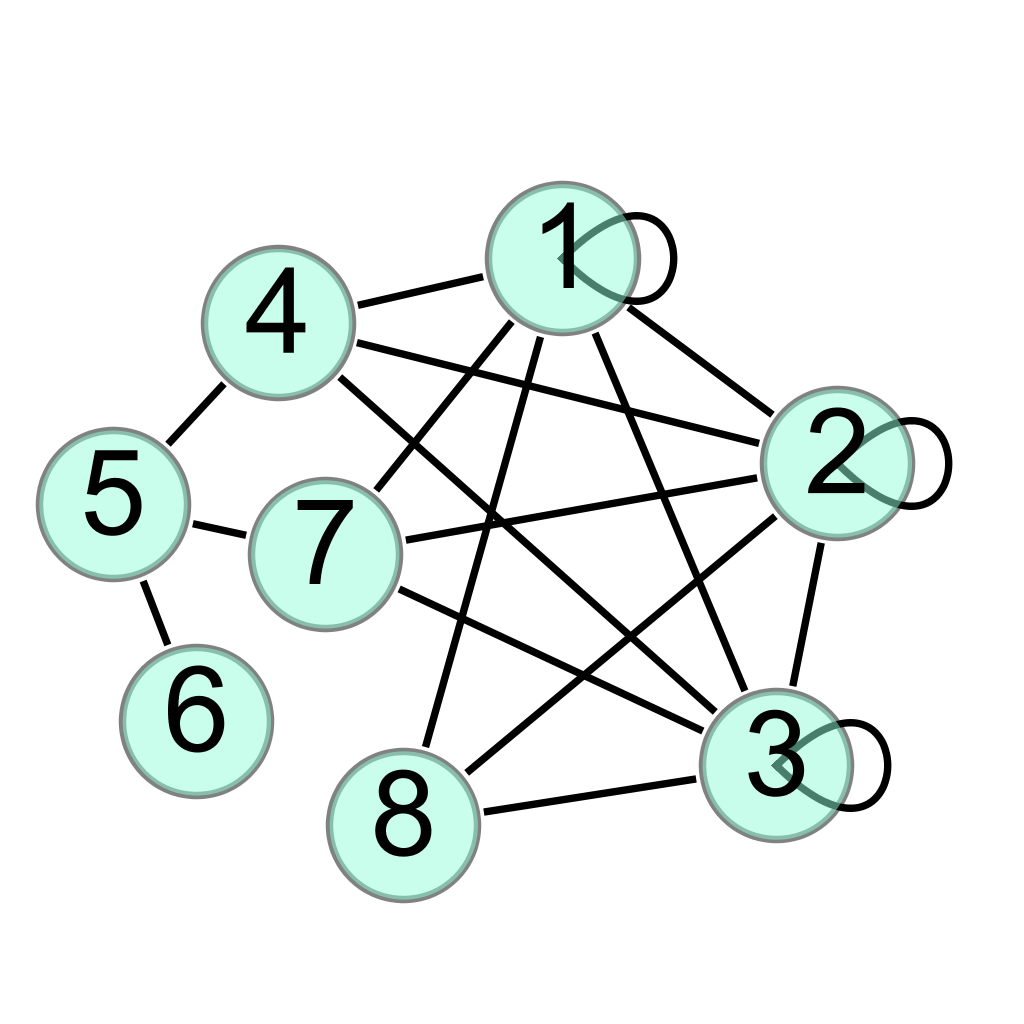
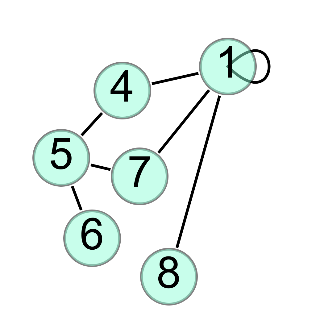
In this section we define a correspondence between $(m,k,s)$ -stars with loops and the $(m,k,s)$ -stars without loops which preserves the eigenvalue spectrum of adjacency and transition matrices. In particular, in a graph, each vertex with a loop is equivalent to an $(1,k,-)$ -star with loop and we will provide a procedure to replace the looped vertex with an $(2,k,s)$ -star without loops which has the same spectra (see Fig.(3)).

The following definitions are useful:

Definition 3.9 ( $(m,k,s)$ -star $q$ -reduced: $S^{\{-q\}}_{m,k,s}$ ).

A $q$ -reduced $(m,k,s)$ -star is a $(m,k,s)$ -star (with or without loops) of vertex sets $\{\mathcal{V}_{1},\mathcal{V}_{2}\}$ , such that the cardinality of $\mathcal{V}_{1}$ is decreased to $m-q$ , with $m>q$ .
Hence the order and degree of the $S^{\{-q\}}_{m,k,s}$ are $m+k-q$ and $m-q-1$ respectively.
Furthermore, let $w$ be the weights between vertexes in the original $(m,k,s)$ -star and $\tilde{i},\tilde{j}$ any vertex in $\mathcal{V}_{1}$ , $\tilde{i}\neq\tilde{j}$ , of the $(m,k,s)$ -star, we define the weights of vertexes in $S^{\{-q\}}_{m,k,s}$ as

w^{\{-q\}}(i,j)=\begin{cases}\frac{q}{m-q}w(\tilde{i},\tilde{j})+w(\tilde{i},\tilde{i}),&\mbox{if }i,j\in\mathcal{V}_{1},\ i=j\\ \frac{m}{m-q}w(\tilde{i},j),&\mbox{if }i\in\mathcal{V}_{1},j\in(\mathcal{V}_{1}\cup\mathcal{V}_{2})\setminus\{i\}\\ w(i,j),&\mbox{if }i,j\in\mathcal{V}_{2}\\ 0&otherwise\end{cases},

(1)

Definition 3.10 ( $(1,k,-)$ -star $q$ -enlarged: $S^{\{+q\}}_{1,k,-}$ ).

A $q$ -enlarged $(1,k,-)$ -star is a $(1,k,-)$ -star (with or without loops) of vertex sets $\{\mathcal{V}_{1},\mathcal{V}_{2}\}$ , such that the cardinality of $\mathcal{V}_{1}$ is increased to $q+1$ and the loop is removed.
Hence the order and degree of the $S^{\{+q\}}_{1,k,-}$ are $1+k+q$ and $q$ respectively.
Furthermore, let $w$ be the weights between vertexes in the original $(1,k,-)$ -star and $\tilde{i}$ the vertex in $\mathcal{V}_{1}$ of the $(1,k,-)$ -star, we define the weights of vertexes in $S^{\{+q\}}_{1,k,-}$ as

w^{\{+q\}}(i,j)=\begin{cases}\frac{1}{q}w(\tilde{i},\tilde{i}),&\mbox{if }i\in\mathcal{V}_{1},j\in\mathcal{V}_{1}\setminus\{i\}\\ \frac{1}{1+q}w(\tilde{i},j),&\mbox{if }i\in\mathcal{V}_{1},j\in\mathcal{V}_{2}\\ w(i,j)&\mbox{if }i,j\in\mathcal{V}_{2}\\ 0&\mbox{if }i=j\in\mathcal{V}_{1}\end{cases},

(2)

Finally we introduce the concept of the $q$ -enlarged graph associate to a graph:

Definition 3.11 ( $q$ -enlarged graph: $\mathcal{G}^{\{+q\}}$ ).

A $q$ -enlarged graph $\mathcal{G}^{\{+q\}}$ is obtained from a graph $\mathcal{G}$ with some $(1,k,-)$ -stars adding $q$ the vertexes in the set $\mathcal{V}_{1}$ of $\mathcal{G}$ , removing the loops and defining the weights as in (2).

Using the previous definitions it is possible to associate to any graph containing $(m,k,s)-star$ with loops (or more simply whose vertexes has a loop), an enlarged graph without loops by means of an intermediate reduced graph as illustrated in Fig.(3). The following theorem holds

Main Theorem 1 (Loop removal theorem - adjacency matrix).

Let

•

$\mathcal{G}$ be a graph, of n vertexes, with a $\accentset{\circ}{S}_{m,k,s}$ ,
•

$\mathcal{H}:=\mathcal{G}^{\{-(m-1)\}}$ be the $(m-1)$ -reduced graph with a $\accentset{\circ}{S}_{m,k,s}^{\{-(m-1)\}}$ instead of $\accentset{\circ}{S}_{m,k,s}$ ,
•

$\mathcal{I}:=\mathcal{H}^{\{+q\}}$ be the $q$ -enlarged graph with a ${S}_{1,k,-}^{\{+q\}}$ instead of $\accentset{\circ}{S}_{1,k,-}$ ,
•

$A$ be the adjacency matrix of $\mathcal{G}$ ,
•

$A^{\{-(m-1)\}}$ be the adjacency matrix of $\mathcal{H}$ , defined as in (1)
•

$A^{\{+q\}}$ be the adjacency matrix of $\mathcal{I}$ , defined as in (2)

then

1.

$\sigma(A^{\{-(m-1)\}})\subset\sigma(A),$
2.

$\sigma(A^{\{-(m-1)\}})\subset\sigma(A^{\{+q\}}),$
3.

There exists a matrix $H\in\mathbb{R}^{n\times(n-(m-1))}$ such that $A^{\{-(m-1)\}}=H^{T}AH$ and $H^{T}H=I$ . Therefore, if $v$ is an eigenvector of $A^{\{-(m-1)\}}$ for an eigenvalue $\mu$ , then $Hv$ is an eigenvector of $A$ for the same eigenvalue $\mu$ .
4.

There exists a matrix $K\in\mathbb{R}^{n-(m-1)\times(n-(m-1)+q)}$ such that $A^{\{-(m-1)\}}=K^{T}A^{\{+q\}}K$ and $K^{T}K=I$ . Therefore, if $v$ is an eigenvector of $A^{\{-(m-1)\}}$ for an eigenvalue $\mu$ , then $Kv$ is an eigenvector of $A^{\{+q\}}$ for the same eigenvalue $\mu$ .

Before proving Theorem 1, we recall the well known result for eigenvalues of symmetric matrices, [Hwa04].

Lemma 3.12 (Interlacing theorem).

Let $A\in Sym_{n_{A}}(\mathbb{R})$ with eigenvalues $\mu_{1}(A)\geq...\geq\mu_{n_{A}}(A).$ For $n_{B}<n_{A}$ , let $K\in\mathbb{R}^{n_{A},n_{B}}$ be a matrix with orthonormal columns, $K^{T}K=I$ , and consider the $B=K^{T}AK$ matrix, with eigenvalues $\mu_{1}(B)\geq...\geq\mu_{n_{B}}(B).$ If

•

the eigenvalues of $B$ interlace those of $A$ , that is,

$\mu_{i}(A)\geq\mu_{i}(B)\geq\mu_{n_{A}-n_{B}+i}(A),\quad i=1,...,n_{B},$
•

if the interlacing is tight, that is, for some $0\leq k\leq n_{B},$

$\mu_{i}(A)=\mu_{i}(B),\ i=1,...,k\ \mbox{ and }\ \mu_{i}(B)=\mu_{n_{A}-n_{B}+i}(A),\ i=k+1,...,n_{B}$

then $KB=AK.$

Proof.

We will explicitly prove only the items 2. and 4., because using the same arguments the statements 1. and 3. follow and the matrix $H$ exists.
First we prove the existence of the $K$ matrix:
let $\tilde{n}:=n-(m-1)$ and $\mathcal{P}=\{P_{1},...,P_{\tilde{n}}\}$ be a partition of the vertex set $\{1,...,\tilde{n}+q\}$ . The characteristic matrix $\tilde{K}$ is defined as the matrix where the $j$ -th column is the characteristic vector of $P_{j}$ ( $j=1,...,\tilde{n}$ ).
Let $A^{\{+q\}}$ be partitioned according to $\mathcal{P}$

A^{\{+q\}}=\left(\begin{array}[]{ccc}A^{\{+q\}}_{1,1}&\dots&A^{\{+q\}}_{1,\tilde{n}}\\ \vdots&&\vdots\\ A^{\{+q\}}_{\tilde{n},1}&\dots&A^{\{+q\}}_{\tilde{n},\tilde{n}}\end{array}\right),

where $A^{\{+q\}}_{i,j}$ denotes the block with rows in $P_{i}$ and columns in $P_{j}$ . The matrix $A^{\{-(m-1)\}}=(a^{\{-(m-1)\}}_{ij})$ whose entries $a^{\{-(m-1)\}}_{ij}$ are the averages of the $A^{\{+q\}}_{i,j}$ rows, is called the quotient matrix of $A^{\{+q\}}$ with respect to $\mathcal{P}$ , i.e. $a^{\{-(m-1)\}}_{ij}$ denotes the average number of neighbors in $P_{j}$ of the vertices in $P_{i}$ .
The partition is equitable if for each $i,j$ , any vertex in $P_{i}$ has exactly $a^{\{-(m-1)\}}_{ij}$ neighbors in $P_{j}$ . In such a case, the eigenvalues of the quotient matrix $A^{\{-(m-1)\}}$ belong to the spectrum of $A^{\{+q\}}$ ( $\sigma(A^{\{-(m-1)\}})\subset\sigma(A^{\{+q\}})$ ) and the spectral radius of $A^{\{-(m-1)\}}$ equals the spectral radius of $A^{\{+q\}}$ : for more details cfr. [BH12], chapter 2.
Then we have the relations

M^{1/2}A^{\{-(m-1)\}}M^{1/2}=\tilde{K}^{T}A^{\{+q\}}\tilde{K},\quad\tilde{K}^{T}\tilde{K}=M.

Considering an $(1,k,-)-$ star (with loop) in a graph with adjacency matrix $A^{\{-(m-1)\}}$ , we weight it by a diagonal mass matrix $M$ of order $\tilde{n}$ whose diagonal entries are one except for the entry of the vertex in $\mathcal{V}_{1}$ ,

M_{ii}=\begin{cases}\frac{1}{1+q},&\mbox{if }i\in\mathcal{V}_{1}\\ 1&\mbox{otherwise }\end{cases},

(3)

and we get

A^{\{-(m-1)\}}=K^{T}A^{\{+q\}}K,\quad K^{T}K=I,

where $K:=\tilde{K}M^{-1/2}.$ In addition to the Theorem (3.5), the eigenvalues of the matrix $A^{\{-(m-1)\}}$ belong also to the spectrum of the matrix $A^{\{+q\}}$ ,

\sigma(A^{\{-(m-1)\}})\subset\sigma(A^{\{+q\}}).

Finally, if $v$ is an eigenvector of $A^{\{-(m-1)\}}$ with eigenvalue $\mu$ , then $Kv$ is an eigenvector of $A^{\{+q\}}$ with the same eigenvalue $\mu$ .
Indeed, from the equation $A^{\{-(m-1)\}}v=\mu v$ and taking into account that the partition is equitable, we have $KA^{\{-(m-1)\}}=A^{\{+q\}}K,$ and

A^{\{+q\}}(Kv)=(A^{\{+q\}}K)v=(KA^{\{-(m-1)\}})v=\mu(Kv).

∎

A similar result holds for the transition matrix $T$ , and more in general for each $D^{-1}A$ where $A$ is the adjacency matrix of the graph $\mathcal{G}$ with a $\accentset{\circ}{S}_{m,k,s}$ and $D$ any real diagonal matrix such that $d_{ii}=d_{jj}$ for any $i,j\in\mathcal{V}_{1}$ . This is states by the following Theorem:

Theorem 3.13 (Loop removal theorem - transition matrix).

Let

•

$\mathcal{G}$ be a graph, of n vertices, with a $\accentset{\circ}{S}_{m,k,s}$ ,
•

$\mathcal{H}:=\mathcal{G}^{\{-(m-1)\}}$ be the $(m-1)$ -reduced graph with a $\accentset{\circ}{S}_{m,k,s}^{\{-(m-1)\}}$ instead of $\accentset{\circ}{S}_{m,k,s}$ ,
•

$\mathcal{I}:=\mathcal{H}^{\{+q\}}$ be the $q$ -enlarged graph with a ${S}_{1,k,-}^{\{+q\}}$ instead of $\accentset{\circ}{S}_{1,k,-}$ ,
•

$A$ and $D$ be, respectively, the adjacency matrix and the strength diagonal matrix of $\mathcal{G}$ ,
•

$A^{\{-(m-1)\}}$ and $D^{\{-(m-1)\}}$ be, respectively, the adjacency matrix and the strength diagonal matrix of $\mathcal{H}$ , defined as in (1)
•

$A^{\{+q\}}$ and $D^{\{+q\}}$ be, respectively, the adjacency matrix and the strength diagonal matrix of $\mathcal{I}$ , defined as in (2)

then

1.

$\sigma(T^{\{-(m-1)\}})\subset\sigma(T),$ where $T^{\{-(m-1)\}}:=(D^{\{-(m-1)\}})^{-1}A^{\{-(m-1)\}}$ and $T:=D^{-1}A$
2.

$\sigma(T^{\{-(m-1)\}})\subset\sigma(T^{\{+q\}}),$ where $T^{\{+q\}}:=(D^{\{+q\}})^{-1}A^{\{+q\}}$
3.

There exists a matrix $H\in\mathbb{R}^{n\times(n-(m-1))}$ such that $T^{\{-(m-1)\}}=H^{T}TH$ and $H^{T}H=I$ . Therefore, if $v$ is an eigenvector of $T^{\{-(m-1)\}}$ for an eigenvalue $\mu$ , then $Hv$ is an eigenvector of $T$ for the same eigenvalue $\mu$ .
4.

There exists a matrix $K\in\mathbb{R}^{n-(m-1)\times(n-(m-1)+q)}$ such that $T^{\{-(m-1)\}}=K^{T}T^{\{+q\}}K$ and $K^{T}K=I$ . Therefore, if $v$ is an eigenvector of $T^{\{-(m-1)\}}$ for an eigenvalue $\mu$ , then $Kv$ is an eigenvector of $T^{\{+q\}}$ for the same eigenvalue $\mu$ .

The proof for the transition matrix version of the Loop removal theorem 1 is similar to that for the adjacency matrix. More explicitly, using the same arguments as in the proof of 1 and the equivalences S.1–S.3 in order to work with symmetric matrices, the items 1. and 2. are true and the matrices $H$ and $K$ exist.

Corollary 4.

Let $\mathcal{G}$ be a graph, of $n$ vertexes, with a $\accentset{\circ}{S}_{m,k,s}$ , if $v$ is a right eigenvector of $T$ with eigenvalue $\lambda\in\sigma(T)\setminus\{\displaystyle-\frac{w_{c}(\accentset{\circ}{S}_{m,k,s})}{w(\accentset{\circ}{S}_{m,k,s})}\}$ then $D^{1/2}v$ is an eigenvector of $\mathcal{L}$ with eigenvalue $(1-\lambda)$ .

The proof directly follows from the Theorem 3.13.

4 Conclusions

The Laplacian matrix associated to undirected graphs provides powerful tools to study the geometrical and dynamical properties of the graph [Big93, Chu97]. In particular, its spectral properties allow to study random walk processes on graphs (e.g. the existence of bifurcation phenomena in the solutions) and to characterize normal modes in a ”springs and masses” interpretation of the graph. The possibility of associating a Laplacian matrix to multigraphs can be a powerful tool in the application of graph theory to network theory in complex system physics, for example in the case of generalized graph Laplacians, in which we can consider both a ”kinetic” and a ”potential” energy term. In a previous work [ARSB18] we have associated the presence of $(m,k)$ -stars in a graph to eigenvalue multiplicity in the Laplacian matrix spectrum. In this work, we have extended the previous results for $(m,k)$ -stars to $(m,k,s)$ -stars with loops. Our approach allows to introduce relations between the spectral properties of adjacency or Laplacian matrices associated to graphs containing $(m,k,s)$ -stars with loops and the spectral properties of corresponding graphs containing only $(m,k,s)$ -stars without loops. This approach allows to extend methods developed for simple graphs also to multigraphs, for example for graph bisection or clustering purposes. The results discussed in the paper allow, firstly, to reduce the size of a graph (with or without loops) preserving the spectral properties and then to describe a graph with loops as a simple graph, without discarding relevant information of the original graph. As a consequence, it is possible to associate to a graph with loops a Laplacian matrix of the reduced graph without loops. Despite the fact that graphs with loops appear in many natural contexts and that they can be obtained by several kinds of aggregation, scaling and blocking procedures, they have not been considered as extensively as simple graphs, since their properties do not verify the conditions required for many theorems on simple graphs. Possible applications of our results could be to organizational networks, where different kinds of ties may appear within the same branch creating loops [Bao08], in citation and co-authorship networks, in which self-citations are possible and the link weights between two authors in co-authorship networks can increase over time if they have further collaborations [BS91, BJN+02], and also in opinion networks, where individuals are subject to vanity [DCH13, QCS14]. Finally, our results could be relevant in neural network models on undirected graphs, where loops tend to freeze the dynamics that makes the system converge toward fixed points [GR15], and to general models of anomalous (sub)diffusion on networks, in which loops represent ”traps” that slow down the systems dynamics [BG90].

Acknowledgments

E. A. thanks Domenico Felice (Max Planck Institute for Mathematics in the Sciences of Leipzig, Germany) for interesting discussions. Part of this work was developed during E. A.’s stay at Max Planck Institute for Mathematics in the Sciences in Leipzig, the author thanks the institution for the very kind hospitality.

References

[AM85] William N. Anderson and Thomas D. Morley. Eigenvalues of the laplacian of a graph. Linear and Multilinear Algebra, 18(2):141–145, 1985.
[ARSB18] Eleonora Andreotti, Daniel Remondini, Graziano Servizi, and Armando Bazzani. On the multiplicity of laplacian eigenvalues and fiedler partitions. Linear Algebra and its Applications, 544:206 – 222, 2018.
[Bao08] Peter. Baofu. The future of information architecture : conceiving a better way to understand taxonomy, network, and intelligence / Peter Baofu. Chandos Oxford, 2008.
[BG90] Jean-Philippe Bouchaud and Antoine Georges. Anomalous diffusion in disordered media. Physics Reports, 195(4):131–160, 1990.
[BH12] Andries E. Brouwer and Willem H. Haemers. Spectra of Graphs. New York, NY, 2012.
[Big93] N. Biggs. Algebraic Graph Theory. Cambridge University Press, 2nd edition, 1993.
[BJN⁺02] A.L Barabási, H Jeong, Z Néda, E Ravasz, A Schubert, and T Vicsek. Evolution of the social network of scientific collaborations. Physica A: Statistical Mechanics and its Applications, 311(3):590 – 614, 2002.
[BLS07] Turker Biyikoglu, Josef Leydold, and Peter Stadler. Laplacien eigenvectors of graphs. Springer, 2007.
[Bon76] John Adrian Bondy. Graph Theory With Applications. Elsevier Science Ltd., Oxford, UK, UK, 1976.
[BS91] Susan Bonzi and H. W. Snyder. Motivations for citation: A comparison of self citation and citation to others. Scientometrics, 21(2):245–254, Jun 1991.
[CH10] Reuven Cohen and Shlomo Havlin. Complex Networks: Structure, Robustness and Function. Cambridge University Press, August 2010.
[Chu97] F. R. K. Chung. Spectral Graph Theory. American Mathematical Society, 1997.
[DCH13] Guillaume Deffuant, Timoteo Carletti, and Sylvie Huet. The leviathan model: Absolute dominance, generalised distrust, small worlds and other patterns emerging from combining vanity with opinion propagation. Journal of Artificial Societies and Social Simulation, 16(1), 2013.
[GR01] C. Godsil and G. Royle. Algebraic Graph Theory, volume 207 of Graduate Texts in Mathematics. volume 207 of Graduate Texts in Mathematics. Springer, 2001.
[GR15] Eric Goles and Gonzalo A. Ruz. Dynamics of neural networks over undirected graphs. Neural Networks, 63:156 – 169, 2015.
[Hwa04] Suk-Geun Hwang. Cauchy’s interlace theorem for eigenvalues of Hermitian matrices. The American Mathematical Monthly, 111(2):157–159, 2004.
[Mer94] Russell Merris. Laplacian matrices of graphs: a survey. Linear Algebra and its Applications, 197:143 – 176, 1994.
[MFR16] Giulia Menichetti, Piero Fariselli, and Daniel Remondini. Network measures for protein folding state discrimination. Scientific Reports, 6:30367:1–8, 2016.
[New10] Mark Newman. Networks: An Introduction. Oxford University Press, Inc., New York, NY, USA, 2010.
[PRP⁺13] Luisa Di Paola, Micol De Ruvo, Paola Paci, Daniele Santoni, and Alessandro Giuliani. Protein contact networks: an emerging paradigm in chemistry. Chemical Review, 113(3):1598–613, 2013.
[PW99] Philippa Pattison and Stanley Wasserman. Logit models and logistic regressions for social networks: $ii$ . multivariate relations. British Journal of Mathematical and Statistical Psychology, 52(2):169–193, 1999.
[QCS14] Walter Quattrociocchi, Guido Caldarelli, and Antonio Scala. Opinion dynamics on interacting networks: media competition and social influence. In Scientific reports, 2014.
[Ray14] Santanu Saha Ray. Graph Theory with Algorithms and Its Applications: In Applied Science and Technology. Springer Publishing Company, Incorporated, 2014.
[Rob13] Garry Robins. A tutorial on methods for the modeling and analysis of social network data. Journal of Mathematical Psychology, 57(6):261 – 274, 2013. Social Networks.
[Sco00] J.P. Scott. Social Network Analysis: A Handbook. SAGE Publications, January 2000.
[Sha15] Termeh Shafie. A multigraph approach to social network analysis. Journal of Social Structure, 16(1):1 – 21, 2015.
[WF94] Stanley Wasserman and Katherine Faust. Social network analysis: Methods and applications, volume 8. Cambridge university press, 1994.

Equivalence between spectral properties of graphs with and without loops

Abstract

1 Introduction

2 Preliminary definitions

3 Definition of (m,k,s)(m,k,s)-star with and without loop

3.1 Eigenvalues multiplicity problem for (m,k,s)(m,k,s)-star

Definition 3.1 ((m,k,s)(m,k,s)-star: Sm,k,sS_{m,k,s} ).

Definition 3.2 (Degree of a (m,k,s)(m,k,s)-star: d​e​g​(Sm,k,s)deg(S_{m,k,s})).

Definition 3.3 (Weight of a (m,k,s)(m,k,s)-star: w⁡(Sm,k,s)w(S_{m,k,s})).

Definition 3.4 (Central weight of a (m,k,s)(m,k,s)-star: wc​(Sm,k,s)w_{c}(S_{m,k,s})).

Theorem 3.5.

Lemma 3.6.

Proof.

Corollary 1.

Corollary 2.

3.2 Eigenvalues multiplicity problem for (m,k,s)(m,k,s)-star with loops

Definition 3.7 ((m,k,s)(m,k,s)-star with loop: S∘m,k,s\accentset{\circ}{S}_{m,k,s} ).

Lemma 3.8.

Corollary 3.

3.3 Correspondence between (m,k,s)-stars with loops and without loops

Definition 3.9 ((m,k,s)(m,k,s)-star qq-reduced: Sm,k,s{−q}S^{\{-q\}}_{m,k,s}).

Definition 3.10 ((1,k,−)(1,k,-)-star qq-enlarged: S1,k,−{+q}S^{\{+q\}}_{1,k,-}).

Definition 3.11 (qq-enlarged graph: 𝒢{+q}\mathcal{G}^{\{+q\}}).

Main Theorem 1 (Loop removal theorem - adjacency matrix).

Lemma 3.12 (Interlacing theorem).

Proof.

Theorem 3.13 (Loop removal theorem - transition matrix).

Corollary 4.

4 Conclusions

Acknowledgments

References

3 Definition of $(m,k,s)$ -star with and without loop

3.1 Eigenvalues multiplicity problem for $(m,k,s)$ -star

Definition 3.1 ( $(m,k,s)$ -star: $S_{m,k,s}$ ).

Definition 3.2 (Degree of a $(m,k,s)$ -star: $deg(S_{m,k,s})$ ).

Definition 3.3 (Weight of a $(m,k,s)$ -star: $w(S_{m,k,s})$ ).

Definition 3.4 (Central weight of a $(m,k,s)$ -star: $w_{c}(S_{m,k,s})$ ).

3.2 Eigenvalues multiplicity problem for $(m,k,s)$ -star with loops

Definition 3.7 ( $(m,k,s)$ -star with loop: $\accentset{\circ}{S}_{m,k,s}$ ).

Definition 3.9 ( $(m,k,s)$ -star $q$ -reduced: $S^{\{-q\}}_{m,k,s}$ ).

Definition 3.10 ( $(1,k,-)$ -star $q$ -enlarged: $S^{\{+q\}}_{1,k,-}$ ).

Definition 3.11 ( $q$ -enlarged graph: $\mathcal{G}^{\{+q\}}$ ).