On Birkhoff’s Theorem in Hořava Gravity

For ${\lambda}=1$, this is the only possible solution of the momentum constraint (6), as in GR case, though not the unique solution for ${\lambda}\neq 1$. However, either ${\lambda}=1$ or ${\lambda}\neq 1$, one can prove $\dot{{\alpha}}^{\prime}=0$, i.e., admitting Birkhoff’s theorem, for generic values of coupling parameters, except one particular set of parameters which relates UV and IR. To prove this, we consider the time derivatives of (5) and (7), which reduce to

where we have used (8) in the last step of (9).

In the presence of the extension term (3), i.e., ${\sigma}\neq 0$, one finds that $\dot{{\alpha}}^{\prime}=0$ is the only possible solution so that Birkhoff’s theorem is satisfied: For the case of $\{\cdots\}=0$ in (9), ${\alpha}(t,r)$ can be integrated as ${\alpha}(t,r)=a(t)+b(r)$ so that $\dot{{\alpha}}^{\prime}=0$ is satisfied again.

On the other hand, in the absence of the extension, i.e., ${\sigma}=0$, (9) gives the usual solution $\dot{{\alpha}}^{\prime}=0$, or an unusual solution for ${\beta}(t,r)$,

which makes $\{\cdots\}=0$ in (9), even without knowing $\dot{{\alpha}}^{\prime}$, where $C$ is an integration constant, which corresponds to the mass for the static case. In general, the second, unusual solution (10) is not compatible with the Hamiltonian constraint (5), which reduces to

However, there exists one exceptional, compatible solution when the conditions

are satisfied.²² 2 Note that, with the conditions in (12), the solution (10) is valid for arbitrary ${\lambda}$, including the ${\lambda}=1$ case: Actually, with $C=0$, the solution corresponds to the zero-mass limit of the ${\lambda}=1$ static black hole solution in [10].

There are two possible solutions for the second condition in (12), i.e., ${\omega}=0$ or ${\omega}=2{\Lambda}_{W}$. The first case, ${\omega}=0$ corresponds to the solution without the IR-modification term [11]. The second case, ${\omega}=2{\Lambda}_{W}$ is the corresponding new solution but, at this time, with the IR modification. A curious property of these solutions is that ${\alpha}(t,r)$ is not constrained by the equations of motions so that ${\alpha}(t,r)$ can be an arbitrary function of space and time. It is this later property that allows the time dependence in the metric and so could violate the Birkhoff’s theorem, even though $\dot{{\beta}}=0$ from (10) and (12). However, we note that these solutions do not have the GR limit, ${\lambda}\rightarrow 1,~{\mu}\rightarrow 0,~{\omega}\rightarrow\infty,~{\Lambda}_{W}\rightarrow\infty$ with ‘ ${\mu}^{2}{\omega},~{\mu}^{2}{\Lambda}_{W}\sim\mbox{fixed}$ ’ [14] so that Birkhoff’s theorem could be violated but only in the non-GR branch.³³ 3 The solution for ${\omega}=0$ seems to be due to the UV detailed balance condition since it does not exist for more generic UV actions [11]. However, the solution for ${\omega}=2{\Lambda}_{W}$ seems to be more generic since one can also obtain the similar solution with modified choice of ${\omega}={\omega}({\Lambda}_{W})$ for more generic UV terms. Another peculiar property of the solution for ${\omega}={\omega}({\Lambda}_{W})$ is that it requires some correlations between IR and UV terms so that only their combined equations have the solution, though separate ones do not.

For ${\lambda}\neq 1$, in addition to the usual solution $\dot{{\beta}}=0$, one may also consider the case of $\dot{{\beta}}\neq 0$ generally, which breaks the Birkhoff’s theorem manifestly from the momentum constraint (6). In order to see whether this is really a feasible solution or not, we need to see whether it is compatible with the Hamiltonian constraints and other field equations. Actually, in this case ${\alpha}(t,r)$ can be determined as

from (6), and be integrated as

with one undetermined, time-dependent function $a(t)$. Then, after some computations with this general solution (14), one can find that Hamiltonian constraint (5) reduces, for the standard case of ${\sigma}=0$,

where we have introduced $f(t,r)\equiv e^{-2{\beta}(t,r)}$ for convenience. Then, (15) and (7) become the equations for $\beta(t,r)$ and $a(t)$. Once we get the solutions for (15), one can prove or disprove the Birkhoff’s theorem by checking whether it can still satisfy the remaining field equation (7), or not. To this ends, instead of getting the explicit solutions for the full equations with both UV and IR parts, which is a formidable task for our case of ${\lambda}\neq 1$, we consider the limiting solutions for the UV and IR equations separately.

First, for the Hamiltonian equation (15) with only the UV terms ($\{\cdots\}$ terms in the right hand side), which corresponds to the limiting case of ${\omega},{\Lambda}_{W}\rightarrow 0$ of the full equation (15), one can solve the equation explicitly and finds that there are two general solutions but only one solution is compatible with the field equation (7), which is given by⁴⁴ 4 In IR region of large $r$, the solution approaches to $f=e^{-2{\beta}}=1$ for ${\lambda}<1$, which is consistent with the case of ${\lambda}=1$ in Sec. A. In other words, there is no discontinuity at the limit ${\lambda}\rightarrow 1_{-}$ in IR, which may be comparable to the Vainshtein mechanism for the massless limit of massive gravity [15]. ,

where ${\epsilon}\equiv\mbox{sign}(3{\lambda}-1)$. This solution is peculiar in that $a(t)$ is unconstrained and there is no integration constant, and this is due to a factorization of an algebraic equation, called Abel’s equation, in the UV limit of ${\omega},{\Lambda}_{W}\rightarrow 0$ [16]. However, from our starting assumption, we find $\dot{{\beta}}\propto\dot{a}\neq 0$, i.e., $a(t)$ can not be trivially a constant so that the solution manifestly violates the Birkhoff’s theorem in the UV regime.⁵⁵ 5 For the case of ${\lambda}=1/3$, where a separate analysis is needed, we find that there is no corresponding time-dependent solution in UV [17]. This is the only result which is qualitatively different from the case of ${\lambda}\neq 1/3$ and it would be probably due to the additional (anisotropic) Weyl symmetry in UV [4, 8].

On the other hand, from the relation (13) or (14), ${\alpha}(t,r)$ is given by

Moreover, it is interesting to note that the solutions (16) and (17) exist only for the de-Sitter branch with a positive cosmological constant ${\Lambda}\propto-{\mu}^{2}>0$, like our current accelerating Universe [18].

Second, for the Hamiltonian equation (15) with only the IR terms (the first two terms in the right hand side), one can also get the explicit solution but find that it is not compatible with the field equation (7) either. So, even for the ${\lambda}\neq 1$ case with an IR Lorentz violation, there is no time-dependent, i.e., Birkhoff’s theorem violating, solution in IR regime.

Finally, with the extension terms in (3), the Hamiltonian equation (15) has additional contributions

where we have introduced $U(t,r)\equiv(ln\dot{{\beta}})^{\prime},~J(t,r)\equiv-2{\beta}^{\prime}$ so that the original PDE problem is reduced to an ODE problem with respect to $r$, with a fixed time $t$. With the extension terms, solving even the IR equation of (15), which actually shows the key role of the extension terms, is a difficult task and its general solution is not available. However, there exists a simple situation that allows an exact solution, which is now compatible with the equation (7) [we will omit the detailed derivation, which is quite cumbersome],

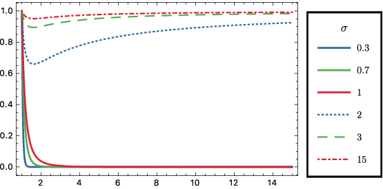
with ${\lambda}=-1,{\Lambda}_{W}=0,{\sigma}=-{\mu}^{2}{\kappa}^{2}{\omega}/8,a(t)=-ln\sqrt{-{\kappa}^{4}{\mu}^{2}{\omega}/64}$ and two arbitrary functions $C_{1}(t)$ and $b(r)$. From our stating assumption of $\dot{{\beta}}\neq 0$, $C_{1}(t)$ can not be just a constant so that this solution violates the Birkhoff’s theorem manifestly even in IR. This situation is quite different from the case of $\dot{{\beta}}=0$ and the other cases of $\dot{{\beta}}\neq 0$ with ${\sigma}=0$, where the violations of Birkhoff’s theorem may occur as the UV effects (or combined UV/IR effects for the case of $\dot{{\beta}}=0$). For other values of parameters, we have obtained the (time-dependent) solutions numerically, by solving about ${\beta}(t,r)$ and $\dot{{\beta}}(t,r)$ using Mathematica. (Fig.1)

In conclusion, we have proved that, for the standard form of Hořava gravity, Birkhoff’s theorem is satisfied in IR for the usual type of solutions which admit the GR limit but can be violated in UV for the unusual type of solutions. In relation to the gravitational radiations, this implies that the scalar gravitons could exist as the results of UV effects but be decoupled in IR regime. Here, it is important to note that we have considered the problems with the full non-linearity by obtaining the exact (time-dependent) solutions for the on-linear equations of motion. This result is consistent with the (fully non-linear) constraint analysis [24], which has been thought to be inconsistent [25, 26], but in contrast to the absence of the scalar gravitons for the whole UV and IR energy ranges in the linear perturbation analyses [19, 20, 21, 22, 23]. This implies a remarkable fact that the UV emergence of time-dependent solutions, i.e., violation of Birkhoff’s theorem, or equivalently scalar gravitons, are the non-linear effect in UV. Actually, if we consider small $a(t)$, the UV time-dependent solution (16), (17) can be expanded as

where $\zeta=1\pm\frac{{\epsilon}\sqrt{-{\kappa}^{4}{\mu}^{2}}}{4|{\lambda}-1|}r^{\frac{-2{\lambda}}{{\lambda}-1}}$. This shows explicitly that, when we consider small $\zeta^{-1}$ as well, $a(t)$ does not appear at the leading, linear orders but emerges only at the sub-leading, i.e., non-linear orders, in consistently with the constraint analysis [24]. [Note that, at the leading order, the $\dot{a}^{2}(t)$ factor in (20) can be removed by redefining the time as $dt\rightarrow dt^{\prime}=dt/\dot{a}(t)$.]

On the other hand, for the extended Hořava gravity with the term of (3), the Birkhoff’s theorem is still satisfied for $\dot{{\beta}}=0$, i.e., $\dot{{\alpha}}^{\prime}=0$ so that there is no time-dependent solutions for the full theory with both the UV and IR terms. However, we have shown an explicit time-dependent solution which violates the theorem in IR for $\dot{{\beta}}\neq 0,~{\lambda}\neq 1$. This is consistent with the perturbative [7] as well as non-perturbative analyses [27] but this seems to be potentially problematic since it implies the existence of gravitational radiations even for pulsating or collapsing, spherically symmetric bodies in IR, which have not been detected yet; even more, it does not reproduce the GR or Newton’s gravity limit in IR, which has been well tested [28].

On the contrary, the existence of a scalar graviton mode, which seems to be represented by a scalar function $a(t)$, indicating the instantaneous mode, in the general solution (14), would have an important role in cosmology. Usually, we need (at least one) primordial scalar matter field, with an instantaneous background, in order to accommodate the observed (nearly scale invariant) scalar power spectrum in CMB data within the inflationary theory [29]. But, now the scalar degree of freedom which is inherent in the non-linear UV regime of Hořava gravity could have a similar role of the primordial scalar field in the early Universe. It would be an outstanding question whether Hořava gravity can provide a consistent framework for the Big Bang cosmology without introducing the artificial primordial scalar field and inflationary scenario [23].

References

- [1] J.T. Jebsen, Ark. Mat. Ast. Fys. (Stockholm) 15, nr. 18 (1921).
- [2] G. D. Birkhoff, Relativity and Modern Physics (Harvard University Press, Cambridge, USA. 1923), p. 253.
- [3] S. Weinberg, Gravitation and Cosmology (Wiley, New York, 1972), pp. 337-338.
- [4] P. Hořava, Phys. Rev. D 79, 084008 (2009).
- [5] C. Charmousis, G. Niz, A. Padilla and P. M. Saffin, JHEP 0908, 070 (2009).
- [6] D. Blas, O. Pujolas and S. Sibiryakov, JHEP 0910, 029 (2009).
- [7] D. Blas, O. Pujolas and S. Sibiryakov, Phys. Rev. Lett. 104, 181302 (2010).
- [8] M. I. Park, Gen. Rel. Grav. 43, 2979 (2011).
- [9] A. Kehagias and K. Sfetsos, Phys. Lett. B 678, 123 (2009).
- [10] M. I. Park, JHEP 0909, 123 (2009).
- [11] H. Lu, J. Mei and C. N. Pope, Phys. Rev. Lett. 103, 091301 (2009)
- [12] E. B. Kiritsis and G. Kofinas, JHEP 1001, 122 (2010).
- [13] A. N. Aliev and C. Senturk, Phys. Rev. D 82, 104016 (2010).
- [14] C. Arguelles, N. Grandi and M. I. Park, JHEP 1510, 100 (2015).
- [15] A. I. Vainshtein, Phys. Lett. 39B, 393 (1972).
- [16] E. Kamke, Differential Gleichungen Losung Methoden und Losungen (Springer Fachmedien Wiesbaden, 1977) p. 373.
- [17] D. O. Devecioglu and M. I. Park, work in progress.
- [18] A. G. Riess et al. [Supernova Search Team], Astron. J. 116, 1009 (1998).
- [19] M. -I. Park, Class. Quant. Grav. 28, 015004 (2011).
- [20] Y. W. Kim, H. W. Lee and Y. S. Myung, Phys. Lett. B 682, 246 (2009).
- [21] X. Gao, Y. Wang, R. Brandenberger and A. Riotto, Phys. Rev. D 81, 083508 (2010).
- [22] J. O. Gong, S. Koh and M. Sasaki, Phys. Rev. D 81, 084053 (2010).
- [23] S. Shin and M. I. Park, JCAP 1712, no. 12, 033 (2017); M. I. Park, EPJ Web Conf. 168, 08003 (2018).
- [24] J. Bellorin and A. Restuccia, Int. J. Mod. Phys. D 21, 1250029 (2012); Phys. Rev. D 83, 044003 (2011).
- [25] M. Li and Y. Pang, JHEP 0908, 015 (2009).
- [26] M. Henneaux, A. Kleinschmidt and G. L. Gomez, Phys. Rev. D 81, 064002 (2010).
- [27] J. Bellorin and A. Restuccia, Phys. Rev. D 84, 104037 (2011).
- [28] R. Reyes et al., Nature 464, 256 (2010).
- [29] A. H. Guth, Phys. Rev. D 23, 347 (1981).