Extremal dependence and spatial risk measures for insured losses due to extreme winds
Abstract
A meticulous assessment of the risk of impacts associated with extreme wind events is of great necessity for populations, civil authorities as well as the insurance industry. Using the concept of spatial risk measure and related set of axioms introduced by Koch, (2017); Koch, (2019), we quantify the risk of losses due to extreme wind speeds. The insured cost due to wind events is proportional to the wind speed at a power ranging typically between and . Hence we first perform a detailed study of the correlation structure of powers of the Brown–Resnick max-stable random fields and look at the influence of the power. Then, using the latter results, we thoroughly investigate spatial risk measures associated with variance and induced by powers of max-stable random fields. In addition, we show that spatial risk measures associated with several classical risk measures and induced by such cost fields satisfy (at least part of) the previously mentioned axioms under conditions which are generally satisfied for the risk of damaging extreme wind speeds. In particular, we specify the rates of spatial diversification in different cases, which is valuable for the insurance industry.
Key words: Extreme wind speed; Insurance; Powers of max-stable random fields; Reinsurance; Spatial diversification; Spatial risk measures and corresponding axioms; Wind damage.
Mathematics Subject Classification (2000): 60F05; 60G60; 60G70; 91B30.
1 Introduction
Extratropical cyclones (such as European windstorms) and tropical cyclones constitute a major risk for society, as can be seen from the consequences in Europe of Windstorms Lothar and Martin in December 1999 (140 fatalities and damage of around 19 billion USD) and, in many Caribbean islands and parts of Florida, of Hurricane Irma in September 2017 (at least 134 deaths and damage exceeding 67.8 billion USD). An accurate evaluation of this risk is essential for civil authorities and the insurance industry.
Having in mind the spatial nature of environmental extreme events, Koch, (2017); Koch, (2019) introduced a new notion of spatial risk measure, which makes explicit the contribution of space and allows one to take into account the spatial dependence of the cost field in the risk measurement. The spatial risk measure associated with a classical risk measure and induced by a cost random field (e.g., modelling the cost due to damage caused by a windstorm) is the function of space resulting from the application of to the normalized integral of on various geographical areas. Koch, (2017); Koch, (2019) also proposed a set of axioms characterising how the value of an induced spatial risk measure is expected to evolve with respect to the space variable, at least under some conditions on and . To the best of our knowledge, the papers by Koch, (2017); Koch, (2019) are the first articles establishing a theory about risk measures in a spatial context where the risks spread over a geographical region. This theory is of interest for the insurance industry as it allows, for instance, the quantification of the rate of spatial diversification.
One of the main goals of the present paper is to apply this notion of spatial risk measure and related axioms to analyze the risk of losses due to extreme wind speeds. We model extreme wind speeds using max-stable random fields (de Haan,, 1984; de Haan and Ferreira,, 2006; Davison et al.,, 2012, e.g.,), which are especially suitable to model the temporal maxima of a given variable at all points in space since they constitute the only possible non-degenerate limiting field of pointwise maxima taken over suitably rescaled independent copies of a random field (de Haan,, 1984, e.g.,). Moreover, we consider the power-law damage function , , for and , which is particularly adapted to wind hazard. Our cost field model arises from the application of to max-stable fields. Although powers equalling or are justified by physical arguments (wind load and dissipation rate of wind kinetic energy, respectively) for the effective cost, it has been shown that they may be much higher when insured costs are considered. For instance, Prahl et al., (2012) find exponents ranging from to for residential buildings in Germany and argue that such large exponents stem for instance from the presence of a deductible in the insurance contract. Hence an important aspect of this paper will be to study how the spatial dependence and risk evolve with respect to that power.
First, we thoroughly investigate the correlation structure of powers of the Brown–Resnick max-stable random field. This part contains new theoretical results for the Brown–Resnick field and, therefore, may be of interest for the extreme-value community independently of any risk-related consideration. Moreover, we perform a numerical study using typical values for the parameters of the generalized extreme-value (GEV) distribution governing annual wind speed maxima, and show that the correlation between damage at two stations basically does not depend on the value of the damage power. This is useful news for insurance companies owing to the large range for possible values of that power. Then, we study several spatial risk measures induced by powers of some max-stable random fields, mainly the Brown–Resnick fields. Using the first part, we theoretically study spatial risk measures associated with variance and induced by such cost fields. This analysis is supplemented with a numerical study where, again, we look at the influence of the value of the power . Moreover, we show that, under conditions which are generally satisfied for the risk of losses due to extreme wind, spatial risk measures associated with several classical risk measures and induced by powers of some max-stable fields satisfy (at least part of) the axioms introduced in Koch, (2017); Koch, (2019). Inter alia, we know the rates of spatial diversification in the cases where the classical risk measures are the variance, the value-at-risk (VaR) and the expected shortfall (ES). The obtained results may have useful implications for the insurance industry and, throughout the study, we keep a strong connection with concrete actuarial practice.
The remainder of the paper is organized as follows. In Section 2, we briefly expose the notion of spatial risk measure and the corresponding set of axioms introduced in Koch, (2017); Koch, (2019). Moreover, we specify the cost field model underlying the examples of spatial risk measures considered; we especially review the literature about wind damage functions and provide a short introduction to max-stable fields. Section 3 investigates the correlation structure of powers of the Brown–Resnick random fields. In Section 4, we study some spatial risk measures induced by those cost fields. Finally, Section 5 provides a short summary as well as some perspectives. Throughout the paper, the elements belonging to for some are denoted by bold symbols, whereas those in more general spaces are designated using normal font. Moreover, stands for the Lebesgue measure in and . Finally, and denote equality and convergence in distribution, respectively. In the case of random fields, distribution has to be understood as the set of all finite-dimensional distributions.
2 Spatial risk measures and cost field model
2.1 Spatial risk measures and corresponding axioms
Let be the set of all compact subsets of with a positive Lebesgue measure and the set of all convex elements of . Denote by the set of all real-valued and measurable11 1 Throughout the paper, when applied to random fields, the adjective “measurable” means “jointly measurable”. random fields on having almost surely (a.s.) locally integrable sample paths. Each field characterizes the economic or insured cost generated by the events belonging to specified categories and occurring during a given time period, say . In the following, is considered as fixed and does not appear for the sake of notational simplicity. Each category of events (e.g., European windstorms or hurricanes) will be named a hazard in the following. Let be the set of all real-valued random variables defined on an adequate probability space. A risk measure is some function and will be referred to as a classical risk measure throughout the paper in order to avoid confusion with a spatial risk measure. A classical risk measure is said to be law-invariant if, for all , only depends on the distribution of .
Koch, (2017); Koch, (2019) introduced the normalized spatially aggregated loss function, defined as
| (1) |
which disentangles the contribution of the space and the contribution of the hazards. The quantity represents the economic or insured loss per surface unit on region due to hazards whose costs can be modelled with the cost field . A spatial risk measure as introduced in Koch, (2017); Koch, (2019) is defined by
where is a classical risk measure. This notion makes explicit the contribution of space in the risk measurement, and, for many useful risk measures such as, e.g., variance, VaR and ES, enables one to take (at least) part of the spatial dependence structure of the field into account. For a given and , the quantity is referred to as the spatial risk measure associated with and induced by . The distribution of only depends on and the finite-dimensional distributions of (Koch,, 2019, Theorem 1). Consequently, for a fixed , if is law-invariant, then only depends on the finite-dimensional distributions of .
Now, let be a classical risk measure, be fixed and, for , let denote its barycenter. Koch, (2017); Koch, (2019) defined the following axioms for the spatial risk measure associated with and induced by , :
- 1.
Spatial invariance under translation: for all and , where denotes the region translated by the vector .
- 2.
Spatial sub-additivity: for all .
- 3.
Asymptotic spatial homogeneity of order : for all ,
where is the area obtained by applying to a homothety with center and ratio , and , are functions depending on .
It is also legitimate to introduce the axiom of spatial anti-monotonicity: for all , . The latter is equivalent to the axiom of spatial sub-additivity. These axioms concern the spatial risk measures properties with respect to space and not to the cost distribution, the latter being fixed. They seem natural and make sense at least under some conditions on the cost field and for some classical risk measures , as shown in Koch, (2017); Koch, (2019). The axiom of spatial sub-additivity qualitatively points out spatial diversification. If it is satisfied with strict inequality, an insurance company would be well advised to underwrite policies in both regions and instead of only one of them. The axiom of asymptotic spatial homogeneity of order quantifies the rate of spatial diversification when the area becomes wide. Hence, knowing might be valuable for the insurance industry.
For more details about these notions and an account of their value for real actuarial practice, see Koch, (2019), Sections 2.1 and 2.2.
2.2 Cost field model for extreme wind speeds
Throughout the paper, we assume the cost to be an insured cost. The general cost field model introduced in Koch, (2017), Section 2.3, is defined by , where is the exposure field, the damage function and the random field of the environmental variable generating risk. Here, the cost is assumed to result from a unique wind hazard (e.g., windstorms, hurricanes, tornadoes) which is characterized by the random field of wind speed extremes over the period , . The application of the damage function to yields the insured cost ratio at each site, which, multiplied by the exposure, gives the corresponding insured cost. For the purpose of this paper, we choose the exposure to be uniformly equal to unity.
We consider, for and , the damage function , which is perfectly suited to the case of wind. Based on physical considerations, the total cost for a specific structure is expected to increase as the square or the cube of the maximum wind speed. Indeed, wind loads and dissipation rate of wind kinetic energy are proportional to the second and third powers of wind speed, respectively. For the square, see, e.g., Simiu and Scanlan, (1996), Equations (4.7.1), (8.1.1) and (8.1.8) and the interpretation following Equation (4.1.20). Regarding the third power, see, among others, Lamb and Frydendahl, (1991, Chapter 2, p.7), where the cube of the wind speed appears in the severity index, and Emanuel, (2005). In his discussion of the paper by Powell and Reinhold, (2007), Kantha, (2008) states that wind damage for a given structure must be proportional to the rate of work done (and not the force exerted) by the wind and therefore strongly argues in favour of the cube rather than the square. In addition to this debate about whether the square or cube is more appropriate for total costs, several studies in the last two decades have found power-laws with much higher exponents when insured costs are considered. For instance, Prahl et al., (2012) found powers ranging from to for insured losses on residential buildings in Germany (local damage functions). Prahl et al., (2015) argue that, if the total cost follows a cubic law but the insurance contract is triggered only when that cost exceeds a positive threshold (e.g., in the case of a contract with deductible), then the resulting cost for the insurance company is of power-law type but with a higher exponent. We have checked this statement using simulations and observed that the resulting exponent depends on the threshold (not shown).
Several authors (Klawa and Ulbrich,, 2003; Pinto et al.,, 2007; Donat et al.,, 2011, e.g.,) use, even in the case of insured losses, a cubic relationship that they justify with the physical arguments given above. However, they apply the third power to the difference between the wind speed value and a high percentile of the wind distribution and not to the effective wind speed; as shown by Prahl et al., (2015, Appendix A3), this is equivalent to applying a much higher power to the effective wind speed.
Due to the various possible values for the right exponent in the damage function (especially depending on the value of the deductible), in this paper we will consider . Without loss of generality, we take , which is consistent with the value we have chosen for the exposure. Note that exponential damage functions are sometimes also encountered in the literature (Huang et al.,, 2001; Prettenthaler et al.,, 2012, e.g.,); we do not consider such functions here.
Furthermore, we take to be a max-stable random field such that the field belongs to , i.e., is measurable and has a.s. locally integrable sample paths. The latter property is satisfied, e.g., as soon as is measurable and the function is locally integrable (Koch,, 2019, Proposition 1). Most often, will be the Brown–Resnick random field (with appropriate margins); see below. As stated in, e.g., Huser and Davison, (2014, Section 2.3), in addition to be very natural models for pointwise maxima, max-stable fields provide appropriate models for extremes of individual observations.
We shall sometimes assume that has standard Fréchet margins; a max-stable field with such margins is said to be simple and will be indicated with “” in superscript. Any simple max-stable random field on can be written (de Haan,, 1984, e.g.,) as
| (2) |
where the are the points of a Poisson point process on with intensity function and the , are independent replications of a random field such that, for all , . The field is not unique and is called a spectral random field of . Conversely, any random field of the form (2) is a simple max-stable field. Now, let be the points of a Poisson point process on with intensity function . Independently, let , be independent replicates of some non-negative random function on satisfying . Then, the mixed moving maxima (M3) random field
| (3) |
is a stationary22 2 Throughout the paper, stationarity refers to strict stationarity. and simple max-stable field. Equations (2) and (3) are useful in practice as they enable the building up of parametric models for max-stable fields, some of which are briefly presented below. Let be a stationary standard Gaussian random field with any correlation function.
Let be a centred Gaussian random field with stationary increments and with variogram , and be defined by , where denotes the variance. Then the field defined by (2) with that is referred to as the Brown–Resnick random field associated with the variogram (Brown and Resnick,, 1977; Kabluchko et al.,, 2009). It is stationary and its distribution only depends on the variogram (Kabluchko et al.,, 2009, Theorem 2 and Proposition 11, respectively). The special case where , , leads to the so-called geometric Gaussian random field (Davison et al.,, 2012, e.g.,). Now, if is written as in (3) with being the density of a -variate Gaussian random vector with mean and positive-definite covariance matrix , it is referred to as the Smith random field with covariance matrix (Smith,, 1990). The Schlather model (Schlather,, 2002) results from taking in (2). Finally, the tube model (preliminary version of Ancona-Navarrete and Tawn, (2002), and Koch, (2017)) arises when taking in (3) , where and .
A commonly used variogram for the Brown–Resnick field is
| (4) |
where and are the range and the smoothness parameters, respectively. An equivalent parametrization of (4) is , where and . The variogram of a random field on with stationary increments is said to be isotropic if, for all , only depends on , where denotes the Euclidean norm. In this case, we associate with the univariate function such that, for all , . In the following we shall mainly focus on the class of Brown–Resnick random fields, which includes the Smith random field. Indeed the Smith field with covariance matrix corresponds to the Brown–Resnick field associated with the variogram
| (5) |
where ′ designates transposition; see, e.g., Huser and Davison, (2013). The variogram in (5) can also be written , where is the norm associated with the inner product induced by the matrix .
The bivariate extremal coefficient function (Schlather and Tawn,, 2003, e.g.,), which is a well-known measure of spatial dependence for max-stable fields, satisfies, for all , , , where is simple max-stable.
In practical applications, max-stable fields are not simple but have GEV univariate marginal distributions with location, scale and shape parameters , and . If is a max-stable field with such GEV parameters, we can write
| (6) |
where is simple max-stable.
Finally, note that other authors considered a similar quantity as (1) within an extreme-value framework, but without cost field and not as a tool to develop a concept of spatial risk measures. For instance, Coles and Tawn, (1996) modelled the so-called areal rainfall using the normalized spatial integral of a max-stable field, Ferreira et al., (2012) investigated the tail properties of the integral over a compact region of a continuous random field in the maximum-domain of attraction of a max-stable field, and Dombry and Ribatet, (2015) proposed the use of the spatial integral of a field to define threshold exceedances in the context of Pareto fields.
3 Correlation of powers of Brown–Resnick fields and applications to wind extremes
3.1 Theory
Several dependence measures for max-stable random fields have been introduced in the literature: the extremal coefficient (Schlather and Tawn,, 2003, e.g.,), the F-madogram (Cooley et al.,, 2006) and the -madogram (Naveau et al.,, 2009), among many others. Here we propose a new spatial dependence measure which is the correlation of powers of max-stable fields and not max-stable fields themselves. More precisely, letting be a max-stable random field with GEV parameters , , , and such that , we focus on
| (7) |
The main motivation for considering this quantity lies in the fact that it can be seen as a measure of spatial dependence for damage due to wind (see Section 2.2) and is thus fruitful for actuarial practice. It may also prove to be useful for the theoretical understanding of max-stable fields and it will be helpful for the study of spatial risk measures associated with variance in Section 4.1. Despite its drawbacks, correlation is commonly used in the finance/insurance industry, making its study useful from a practical point of view. Furthermore, the criticism that it does not properly capture extremal dependence is somehow irrelevant here as we consider the correlation between random variables which already model extreme events.
The purpose of this section is the study of in the case of the Brown–Resnick random field. Owing to the wide range of possible values for the damage power , its sensitivity with respect to will also be considered. The Brown–Resnick field is one of the most (if not the most) suitable models among currently available max-stable models, at least for environmental data (e.g., Davison et al.,, 2012, Section 7.4, in the case of rainfall). Notably, it allows realistic realizations as well as independence when distance goes to infinity.
From (6), we know that any max-stable field with general GEV margins can be expressed as a function of a simple max-stable field. Hence, we first consider simple max-stable fields as they are easier to handle. The following lemma is immediate and thus the proof is omitted.
Lemma 1.
Let and be a random variable following the standard Fréchet distribution. Then has a finite first moment if and only if (iff) and a finite second moment iff . Moreover, , where denotes the gamma function.
For , we introduce the function defined by
| (8) |
where, for ,
with and denoting the standard Gaussian distribution and density functions, respectively. We denote by the covariance. The following result will help us a lot to derive the expression of .
Theorem 1.
Let be a simple Brown–Resnick random field associated with the variogram . Then, for all and , we have
| (9) |
Proof.
Let and .
First, we show the result in the case where . Since is simple max-stable, it follows from Lemma 1 that
which yields (9) as .
Now, we prove the result in the case where are distinct vectors of . We have
where denotes the bivariate density of the Brown–Resnick field (at and ). In order to take advantage of the radius/angle decomposition of multivariate extreme-value distributions, we make the change of variable
The corresponding Jacobian matrix is written
and its determinant is thus . Therefore, introducing
we have
| (10) |
Let . Equation (4) in Padoan et al., (2010) gives that the bivariate density of the Smith random field (at and ) satisfies, for ,
| (11) |
where
It is known that the bivariate distribution function (at ) of the Brown–Resnick random field associated with the variogram is the same as that of the Smith random field with covariance matrix when replacing with ; compare Equation (1) in Huser and Davison, (2013) and Equation (3) in Padoan et al., (2010). It follows that the bivariate density (at and ) of the Brown–Resnick field associated with the variogram is given by the right-hand side of (11) with being replaced with . Therefore, for any ,
| (12) |
We denote by the Fréchet distribution with shape and scale parameters and , i.e., if , Using (10) and (12) and the fact that the density of is written , we obtain
| (13) |
where stands for the -th moment of a random variable having as distribution. It is immediate to see that , which, combined with (13), yields the result. ∎
We now aim at studying our spatial dependence measure . The next result, that we derive from Theorem 1 constitutes an important step in that direction.
Theorem 2.
Let and be a Brown–Resnick field with GEV parameters , and at , . Moreover, let such that , . Then, we have
where
Proof.
The following is an immediate consequence of Theorem 2.
Corollary 1.
Our dependence measure is given by the ratio of the right-hand-sides of (14) and (15). In order to derive useful conclusions about , we investigate the behaviour of the function defined in (16). For this purpose, we first need the following result.
Proposition 1.
For a random vector , its distribution function is denoted . Let and be random vectors having the same margins. Then, we have
for all strictly increasing functions and , provided the covariances exist.
Proof.
The proof is partly inspired from the proof of Theorem 1 in Dhaene and Goovaerts, (1996). Let and be strictly increasing functions. Assume that, for all ,
| (17) |
We have
and the same equality for . Consequently, since, for all , , it follows from (17) that, for all ,
| (18) |
Since and have the same distribution and the same is true for and , we deduce that
| (19) |
For a random variable , we denote by its distribution function. Using (18), (19) and Lemma 1 in Dhaene and Goovaerts, (1996), we obtain
∎
Henceforth, we can show the following technical result which will be used below.
Proposition 2.
For all , , and such that , the function defined in (16) is strictly decreasing.
Proof.
Let be the simple Smith random field with covariance matrix , which is a Brown–Resnick random field associated with the variogram . Let . Equation (3.1) in Smith, (1990) gives that, for all ,
where . We immediately obtain that
| (20) |
where
For all , we introduce , which is positive. We have
which is negative. Thus, (20) gives that, for all and ,
| (21) |
Let us consider and , , , such that
| (22) |
It follows from (21) that, for all , . Since is simple max-stable, we have and . Now, as , for , the function
is strictly increasing. Hence, letting
Proposition 1 yields
| (23) |
Furthermore, we know from (14) that, for all satisfying ,
| (24) |
Finally, the combination of (22), (23) and (24) gives that , showing the result. ∎
The two following propositions especially give the behaviour of the function around and at .
Proposition 3.
For all , , and such that , the function defined in (16) satisfies
| (25) |
and is continuous everywhere on .
Proof.
Let be the Smith random field with covariance matrix , where is the identity matrix in dimension 2, and with GEV parameters , and . The field is stationary by stationarity of . In addition, as , we know from Lemma 1 that has a finite second moment. Accordingly, is second-order stationary. Moreover, since the Smith random field is sample-continuous, it immediately follows that is sample-continuous and thus, using the same arguments as in the proof of Proposition 1 in Koch et al., (2019), that it is continuous in quadratic mean. Hence, the covariance function of the field is continuous at the origin. This implies, using (14), that
which, combined with (15), yields (25). This easily gives , which implies that is continuous at . The continuity of at any comes from the fact that the covariance function of a field which is second-order stationary can be discontinuous only at the origin. ∎
Proposition 4.
For all , , and such that , the function defined in (16) satisfies
| (26) |
Proof.
Let be the Smith random field with covariance matrix , and with GEV parameters , and . As will be seen in the proof of Theorem 6, the field satisfies the central limit theorem (in a sense specified in Section 4.2). This implies (see Section 4.2) that
which entails, using (14), that
Since is strictly decreasing, this necessarily implies that
i.e., (26). ∎
We have assumed throughout this section that but, as shown by the next proposition, the case is easily recovered by letting tend to in the expressions above.
Proposition 5.
Let , , and define
where is a simple max-stable random field. Let such that there exists satisfying . Then, we have, for all ,
Proof.
For , follows the GEV with parameters , and , the density of which we denote by . For , we easily obtain for any , and, for , we have for all
It is easy to see that the first integral is finite and that the only possible problem for the existence of the second one is at . We have
where we used the change of variable . As , the previous integral is finite provided , which yields by assumption that . Now, let , , and . By Cauchy-Schwarz inequality,
which gives . It follows from Billingsley, (1999, p.31) that the , and are uniformly integrable for around .
Now, it is well-known that , , which implies by the continuous mapping theorem that . Moreover, for any ,
and
where is the exponent function of . Thus,
and thus
Consequently, the continuous mapping theorem yields
and hence, applied again, . Finally, Theorem 3.5 in Billingsley, (1999) yields that , and . The result follows immediately. ∎
Using similar arguments, we can show that , , which yields, for any ,
3.2 Application
The expression of depends on and through only; accordingly, we use in the following the notation . Below, we study the behaviour of with respect to and the Euclidean distance for different variograms. As a variogram is a non-negative conditionally negative definite function, it follows from Berg et al., (1984, Chapter 4, Section 3, Proposition 3.3)33 3 In that book, the term “non negative” is used for “conditionally non negative”. that , , defines a metric. For many common models of isotropic variogram , is a strictly increasing function of , which implies by (14) and Proposition 2 that is a strictly decreasing function of ; such a decrease of the correlation with the distance seems natural. Moreover, (14), (15) and (25) give that . Now, introducing , for a function from to , must be understood as . Using (14) and (26), we deduce, provided that , that . Furthermore, the faster the increase of to infinity, the faster the convergence of to . These results are consistent with our expectations.
We now thoroughly study the evolution of with respect to and , for fixed values of the GEV parameters , and . As we want our study to be closely linked to practice, we choose reasonable values of those GEV parameters. Fitting a generalized Pareto distribution (GPD) to in situ observations over Switzerland, Ceppi et al., (2008) obtained a shape parameter ranging from to . Della-Marta et al., (2007) fitted the GPD to ERA-40 reanalysis data over Europe during windstorms and also found negative shape parameters, with values between and on most of land areas; see their Figure 4.15. More generally, many studies point out that is generally slightly negative, entailing that the distribution of wind speed maxima has a finite right endpoint; when a positive value is obtained, it is never too far from . In the case of annual maxima over Europe, classic values for the location parameter lie between and m.s-1 and usual values of the scale parameter range from to m.s-1. E.g., considering annual maxima wind speeds at 35 weather stations in the Netherlands, Ribatet, (2013) obtained trend surfaces whose intercepts are about m.s-1 for and m.s-1 for . We considered the m wind gust ERA-5 reanalysis data on a rectangle over France from to longitude and to latitude (basically centred in Paris). Fitting the GEV to annual maxima of these data, the mean estimates computed on the 77 grid points are m.s-1, m.s-1 and . Due to these various results, we perform our study with the values , and for simplification; the results described below remain qualitatively the same with different values of these parameters.
The integral appearing in the expression of (see (8)) has no closed form and therefore a numerical approximation is required. For this purpose, we use adaptive quadrature with a relative accuracy of . Furthermore, we choose the variogram (4) with and . A value of the smoothness parameter between and seems reasonable for wind speed maxima; e.g, Ribatet, (2013) obtained and on similar data, Einmahl et al., (2016) found , whereas we get on the region described above and over a region covering the Ruhr in Germany (the numbers inside the brackets denote the standard deviation). The difference may come from the fact that reanalysis tend to be smoother than in situ observations. Choosing a range does not induce any loss of generality in our study as, should differ from , the appropriate plots would be the same as below with the values on the x-axis multiplied by . In practical situations, the true value of should of course be taken. From (5), we know that the case corresponds to the Smith field with . Finally, the cases and are intermediate between the two previous settings. In accordance with the discussion above, Figure 1 shows that decreases from to as the Euclidean distance increases, and this at a higher rate for larger values of . Especially, the decrease is faster for the Smith field than for all Brown–Resnick fields having , and if the true value of is close to or even , using the Smith model leads to a serious underestimation of the dependence between damage. The minimum Euclidean distance required for to be lower than is about for (not shown), instead of around for . Moreover, interestingly, for a given Euclidean distance, slightly increases in a concave way with the power but is basically constant, suggesting that our dependence measure is only faintly sensitive to the value of . On top of being potentially insightful for the understanding of max-stable fields, this finding is valuable for actuarial practice as it means that the correlation between damage due to extreme wind speeds is basically the same whatever the value of the power. It also makes sense to consider the extension of (7) where the relevant damage power is at and at with and not necessarily equal, as in Theorem 2. The behaviour is fairly similar to what we just described (not shown). Especially, for a given distance, the values are not highly sensitive to the combination . For a fixed , the correlation first increases and then decreases with , but the value of achieving the maximum increases to as increases to . Moreover, the higher the values of , the higher the sensitivity with respect to . The evolution of the covariance with respect to the distance is similar as for the correlation, but the sensitivity with (or the combination in the extension just mentioned) is much larger, owing to the non-normalized nature of covariance.
4 Spatial risk measures induced by powers of max-stable fields and applications to wind extremes
In this section, we study some examples of spatial risk measures induced by the cost field
| (27) |
where is a max-stable random field belonging to with GEV parameters , , and the power satisfies or . Most often, will be the Brown–Resnick random field. As before, we keep a tight connection to concrete applications to the risk of losses due to extreme wind speeds.
We shall use the following lemma.
Lemma 2.
Let be a measurable max-stable random field with GEV parameters , and . Let such that . Then, the random field belongs to .
Proof.
The field is obviously measurable. Furthermore, as has identical univariate marginal distributions, the function is constant and hence locally integrable. Therefore, Proposition 1 in Koch, (2019) yields that has a.s. locally integrable sample paths. ∎
Let and be as in Lemma 2. We consider the field and the spatial risk measure associated with the expectation . It is clear that is measurable. In addition, since it has identical univariate marginal distributions and , it has a constant expectation and, for any , . Consequently, Theorem 3 in Koch, (2019) gives that, for all , and that satisfies the axioms of spatial invariance under translation and spatial sub-additivity. Provided that , it also yields that satisfies the axiom of asymptotic spatial homogeneity of order with and , . Using (6), the binomial theorem and Lemma 1, we obtain
| (28) |
Spatial risk measures associated with the expectation are not of great interest since, by Fubini’s Theorem, they do not account for the spatial dependence of the cost field . In the following, we study some spatial risk measures associated with variance in detail. Then, we provide a central limit-based approximation of the distribution of for and large enough. Finally, we analyze some spatial risk measures associated with VaR and ES. For a discussion about the respective advantages and drawbacks of variance, VaR and ES as classical risk measures, we refer the reader to Koch, (2019, Section 3).
4.1 Spatial risk measures associated with variance
We focus on , provided it is finite, where is given in (27). We first study in detail the function for specific regions . Among others, we derive useful expressions for , , that may be of practical relevance for the insurance industry and will allow us to prove the axiom of spatial sub-additivity in specific configurations. Second, we provide conditions on the field such that satisfies (at least) part of the axioms presented in Section 2.1.
4.1.1 Study of
Let be a measurable max-stable random field with GEV parameters , and . Moreover, let such that and . Lemma 2 yields that and it easily follows from Lemma 1 that, for all , . Thus, using Theorem 4 in Koch, (2019), we obtain that, for all and ,
| (29) |
Hence, taking advantage of the expression of obtained in (14), we deduce the expression of in the case where is the Brown–Resnick random field with an isotropic variogram and when the region is a disk or a square. In the whole paper, disk and square refer to a closed disk with positive radius and a (closed) square with positive side, respectively. The corresponding results are given in the next theorem.
Theorem 3.
Let be a measurable Brown–Resnick random field associated with an isotropic variogram whose corresponding univariate function is and with GEV parameters , and . Let such that and . Then:
- 1.
Let be a disk with radius . For all , we have
(30) where is the density of the Euclidean distance between two points independently and uniformly distributed on , given, for , by
- 2.
Let be a square with side . For all , we have
where is the density of the Euclidean distance between two points independently and uniformly distributed on , written as
with .
Proof.
Using (14), we obtain, for ,
The results follow from (29) and similar arguments as in the proof of Corollary 1 in Koch, (2017). ∎
Let and as in Proposition 5, and . Using Cauchy–Schwarz inequality, we can easily apply the Lebesgue dominated convergence theorem to show that
Therefore, again, the case is recovered by letting tend to .
The following theorem concerns the limit of as .
Theorem 4.
Let , and be as in Theorem 3 and assume moreover that is measurable and satisfies
| (31) |
Then, for all being a disk with radius or a square with side , .
Proof.
We show the result when is a disk; the arguments are the same in the case of the square. Since is a continuous function of on , it is bounded. By Propositions 2–4, is also bounded and consequently there exists such that, for all and , . In addition, and are continuous and thus measurable, which yields by measurability of that, for all , the function is measurable. Thus, by Lebesgue’s dominated convergence theorem, the fact that is a density and (31),
| (32) |
Finally, combining (26), (30) and (32), we obtain
∎
Let and be as in Theorem 3. If the function is strictly increasing (respectively increasing), then Proposition 2 implies that, for all , the function is strictly decreasing (respectively decreasing). Therefore, it follows from Theorem 3 that is strictly decreasing (respectively decreasing) for being a disk or a square; there is thus spatial diversification. Furthermore, if is measurable and satisfies (31), Theorem 4 entails that this spatial diversification is total, which has to be understood in the sense that . Theorem 3 is of interest for the insurance industry as it allows a company to compute the value of such that equals a wanted low variance level. In other words, it enables one to find out the characteristic dimension of a geographical area needed to reach a specified low variance for the loss per surface unit.
Below, we study how evolves with respect to under the assumptions of Theorem 3 for various values of . The integrals involved have no closed form and thus, as above, we use adaptive quadrature with as relative accuracy. We set without loss of generality and, as in Section 3, we choose , , , and consider the variogram , , with ; similar results are obtained with different marginal parameters. Figure 2 displays a rapid decrease to in the case (blue curve) which corresponds to the Smith random field; the decrease is somewhat slower in the case of the square. This behaviour is similar to the one observed when the cost field is the indicator function of the Smith random field exceeding a given threshold; see Koch, (2017), Figure 1. Figure 2 also shows that, for a fixed , the decrease to becomes much slower when decreases, which was theoretically expected since the rate of convergence to raises as the rate of divergence of the variogram to infinity increases. Again, an insurance company that would model wind speed extremes using the Smith model would substantially underestimate its risk if the true value of is less than . The curves are very similar for other values of , but for a given the value of increases basically exponentially with ; the plot of with respect to is essentially linear (not shown). This feature is comprehensible in view of the expression of and the evolution of the function with respect to (see Figure 3 in Appendix A). Hence, although the value of has little impact on the spatial dependence measure , it strongly influences the values of , . As in Section 3, choosing a range different from would not affect our conclusions. It would just modify the values on the x-axis: the larger the range, the slower the spatial diversification.
4.1.2 Axioms
We start with a preliminary result. Let and denote the Borel -fields on and , respectively.
Lemma 3.
Let be a simple max-stable random field. Let , , and . The function defined by
| (33) |
is measurable from to and strictly increasing. Moreover, if , then for any such that .
Proof.
The fact that is measurable and strictly increasing is obvious. Denoting , we have, for ,
which is finite (see the proof of Proposition 5) provided as follows the GEV with parameters , and . The latter inequality is satisfied for any positive such that . ∎
We shall use the following remark.
Remark 1.
It is easily seen that Theorem 3 in Koch et al., (2019) also holds true if is a simple Brown–Resnick field with variogram (and not only ), where , and is any symmetric positive-definite matrix; this implies that Theorem 8 and Corollary 4 in Koch, (2019) are also true in this more general setting. In the following, when we refer to Theorem 8 and Corollary 4 in Koch, (2019), we refer to this extended version.
The following theorem provides conditions on the field such that satisfies (at least) part of the axioms in Section 2.1.
Theorem 5.
- 1.
Let be a stationary and measurable max-stable random field with GEV parameters , and . Let such that . We introduce the cost field . Then, the spatial risk measure induced by satisfies the axiom of spatial invariance under translation. In particular, this is true for the tube random field as well as the measurable Schlather and Brown–Resnick fields (which includes the Smith field).
- 2.
Let be a measurable Brown–Resnick random field associated with an isotropic variogram such that is increasing and with GEV parameters , and . Let such that and . Then satisfies the axiom of spatial sub-additivity when the two regions are both a disk or a square. The axiom is satisfied with strict inequality if is strictly increasing, as in the case of the isotropic Smith field.
- 3.
Let be the Brown–Resnick random field associated with the variogram , , where , and is any symmetric positive-definite matrix. Assume that the GEV parameters of are , and . Let such that and . Then satisfies the axiom of asymptotic spatial homogeneity of order , with
where the expression of , , is given by (14).
Proof.
1. By Lemma 2, . Moreover, since is stationary, it is also the case for . Additionally, as mentioned immediately before (29), the induced spatial risk measure is well-defined. Finally, Var is a law-invariant classical risk measure. Hence, Theorem 5, Point 1, in Koch, (2019) gives the first result. As an instance of moving maxima random field, the tube model is stationary and measurable. Hence, the specific fields mentioned satisfy the assumptions, concluding the proof.
2. First, is invariant under translation by Point 1. Moreover, for being a disk or a square, we have seen in Section 4.1.1 that is decreasing (respectively strictly decreasing) if is increasing (respectively strictly increasing). Therefore, the result follows by the same reasoning as in the proof of Theorem 3, Point 2, in Koch, (2017).
3. It follows from (6) and (33) that , where is simple max-stable. Lemma 3 gives that satisfies the assumptions of Corollary 4 in Koch, (2019). Thus, the result directly follows from Corollary 4 in Koch, (2019). ∎
In the case of damage caused by extreme wind speeds, the condition is generally satisfied for any since, most often, . When , the corresponding value is typically very close to and this condition is satisfied for low to moderate powers. Hence, in concrete applications, the results of Theorem 5 usually hold true.
Remark 2.
We think intuitively that Point 2 of Theorem 5 is also true for all or even and not only for disks and squares. However, it is difficult to prove it with the current argument based on the expressions of of Theorem 3 as, for more complex geometric shapes of the region , little is known on the density of the distance between two points independently and uniformly distributed on (e.g., Moltchanov,, 2012, Section 4.3.3).
Remark 3.
Let have GEV parameters , and . Furthermore, let such that . The result of Theorem 5, Point 3, is also true if is a sample-continuous Brown–Resnick random field associated with a variogram which satisfies the slightly weaker condition
| (34) |
for some satisfying .
Proof.
The field is sample-continuous and thus measurable, which yields by Lemma 2 that . By stationarity of the Brown–Resnick field, for all , . Now, it follows from (6) and (33) that , where is a simple and sample-continuous max-stable field. Lemma 3 gives that and that satisfies the requirements for in Proposition 1 in Koch et al., (2019). The latter yields . Denoting by the extremal coefficient of the Brown–Resnick field, (34) precisely means that . Finally, the result follows from Theorem 6 in Koch, (2019). ∎
4.2 Central limit theorem and homothety
We first recall the concepts of Van Hove sequence and central limit theorem (CLT) for random fields on . For and , we denote , where stands for the Euclidean distance. Additionally, we denote by the boundary of . A Van Hove sequence in is a sequence of bounded measurable subsets of satisfying , , and . We say that a random field such that, for all , , satisfies the CLT, if
and, for any Van Hove sequence in ,
where denotes the normal distribution with expectation and variance .
Using results about CLT for functions of stationary max-stable random fields by Koch et al., (2019) and an outcome of Koch, (2019), we obtain the following theorem.
Theorem 6.
Proof.
Such a Brown–Resnick random field is sample-continuous (Koch et al.,, 2019, proof of Theorem 3) and thus measurable, which yields by Lemma 2 that . Moreover, is stationary and therefore has a constant expectation. In addition, by Lemma 3, satisfies the assumptions on the function of Theorem 3 in Koch et al., (2019). Thus, the latter theorem yields that satisfies the CLT. Finally, (28) yields . The result follows from Theorem 2 in Koch, (2019). ∎
If is large enough, this result gives an approximation for the distribution of the normalized spatially aggregated loss:
where means “approximately follows”. Such an approximation is useful in practice, e.g., for an insurance company. For the same reasons as those mentioned in Section 4.1.2, these results generally hold true when the focus in on damage due to extreme wind speeds.
4.3 Spatial risk measures associated with value-at-risk and expected shortfall
For a random variable with distribution function , its value-at-risk at confidence level is written . Moreover, provided , its expected shortfall at confidence level is defined by
Classic values for are and . In the actuarial literature, ES is sometimes referred to as tail value-at-risk (e.g., Denuit et al.,, 2005, Definition 2.4.1). In the following, for , and denote the quantile at level and the density of the standard Gaussian distribution, respectively. In this section, we focus on
where and is given in (27). We first shortly comment on the functions and , for , and then provide conditions on the field such that and satisfy (at least partially) the axioms in Section 2.1.
4.3.1 Study of and ,
Deriving a tractable formula for VaR of , , is very difficult. The same type of approximation as that described in Koch, (2017, Section 4.3.1) can be used, leading to similar graphs as Figure 6 in Koch, (2017) for the function , but this approach is numerically rather time-consuming.
For the same reasons, it is arduous to obtain a tractable formula for ES of , . Nonetheless, as
| (36) |
for a continuous random variable , it is possible to approximate ES of by estimating the right-hand side of (36) with a Monte-Carlo method; this is however time-consuming.
4.3.2 Axioms
We do not have an explicit formula for and , but outcomes from Koch, (2019) (connected with Theorem 6) yield their asymptotic behaviours (when ) under some conditions. The corresponding result is part of next theorem.
Theorem 7.
- 1.
Let be a stationary and measurable max-stable random field with GEV parameters , and . Let and such that has a.s. locally integrable sample paths (this is satisfied, e.g., if ). Then, for all , satisfies the axiom of spatial invariance under translation. Provided , the same is true for . These results hold true, e.g., for the tube random field and the measurable Schlather and Brown–Resnick fields (including the Smith field) if .
- 2.
Proof.
1. The field belongs to by assumption and is stationary by stationarity of . The fact that has a.s. locally integrable sample paths when directly follows from Lemma 2. Now, is well-defined. In addition, we have, for all , that
Accordingly, if , the stationarity of and Fubini’s theorem entail that , which implies that is well-defined. Finally, VaR and ES are both law-invariant classical risk measures. Consequently, Theorem 5, Point 1, in Koch, (2019) gives the first result. The end of the proof of Theorem 5, Point 1, and the fact that implies show that the specific fields mentioned satisfy the required assumptions, concluding the proof.
2. The arguments are the same as in the proof of Theorem 5, Point 3. ∎
As above, these results generally hold true in the case of the risk of extreme wind speeds.
Remark 4.
The results of Theorem 5, Point 3, Theorem 6 and Theorem 7, Point 2, hold true for a more general Brown–Resnick field, more specifically satisfying the conditions of Remark 3 in Koch et al., (2019) or, equivalently, Theorem 9 in Koch, (2019).
5 Conclusion
As detailed in the paper, literature suggests that power-laws are appropriate wind damage functions but that the suitable power varies significantly from a situation to the other, most often from to ; especially it is an increasing function of the deductible of the insurance contract. Thus, the study of powers of extremal fields is insightful for the assessment of the risk of losses due to extreme wind speeds, and analyzing the sensitivity to the value of the power is needed. In this paper, we thoroughly investigate the correlation structure of powers of the Brown–Resnick max-stable random field, which is a very suited model for spatial extremes. Even if our primary focus is on risk assessment of damaging wind speeds, the obtained results may be valuable for the extreme-value community regardless of any notion of risk. Then, we illustrate the concepts of spatial risk measure and corresponding axioms introduced in Koch, (2017); Koch, (2019) in a context where the cost fields are precisely powers of max-stable fields. Using the previous part, we perform a comprehensive study of spatial risk measures associated with variance and induced by such cost fields. In addition, we show that under relatively mild conditions which are typically satisfied for the risk of damaging extreme wind speeds, the induced spatial risk measures associated with several classical risk measures satisfy (at least part of) the axioms. Variance, VaR and ES lead to asymptotic spatial homogeneity of order , and , respectively. Our results are valuable for risk assessment in actuarial practice of, e.g., extratropical and tropical cyclones.
Ongoing work consists, inter alia, in applying the results of the current paper to the pricing of concrete reinsurance treaties as well as event-linked securities such as catastrophe bonds.
Acknowledgements
The author wishes to thank Anthony C. Davison, Paul Embrechts, Pierre Ribereau and Christian Y. Robert for some comments. He also would like to acknowledge the MIRACCLE-GICC project, RiskLab at ETH Zurich, the Swiss Finance Institute, the Swiss National Science Foundation (project 200021_178824) and the Institute of Mathematics at EPFL for financial support.
Appendix A Case of simple max-stable random fields and or
This appendix explains that the results obtained above basically apply if the max-stable random field is simple (instead of having general GEV margins) and or . The point is that is allowed to take any value below these upper bounds and does not need to be an integer anymore. As standard Fréchet margins are far from being realistic for wind speed extremes, the interest of this section mostly lies in a better understanding of some properties of max-stable fields.
First we consider the dependence measure , where is a simple Brown–Resnick max-stable random field and , i.e., . The condition with of (7) translates into ; any negative value is allowed as simple max-stable fields are a.s. positive. We introduce, for ,
which arises when setting in the function specified in (8). Denoting by the variogram of , it follows from Theorem 1 that, for all and , . Our dependence measure (provided that ) is readily derived and its behaviour is similar to the one we observed in Section 3 (not shown).
We now investigate the function in further details. Very similar proofs as for Propositions 2–4 yield, for , that the functions defined in (8) and are strictly decreasing, (implying that is continuous everywhere on ) and . This entails that, for any , . Figure 3, obtained using adaptive quadrature with a relative accuracy of , shows that the decrease of for a given with respect to is more and more pronounced when increases, and that, for fixed, the absolute value of the slope of increases very fast with , in link with rapid divergence to . Obviously, the behaviour of is similar; the same holds true for .
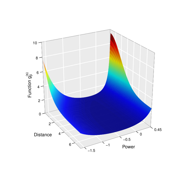
The next theorem gives the expression of when is a simple Brown–Resnick random field with an isotropic variogram, is either a disk or a square, and .
Theorem 8.
Let be a measurable simple Brown–Resnick random field associated with an isotropic variogram whose corresponding univariate function is . Let and . Finally, let and be as in Theorem 3. Then:
- 1.
Let be a disk with radius . For all , we have
- 2.
Let be a square with side . For all , we have
We also have the equivalent of Theorem 4.
Theorem 9.
Let , and be as in Theorem 8. Furthermore, assume that is measurable and satisfies
Then, for all being a disk with radius or a square with side , .
Theorem 9 is consistent with the current knowledge about mixing of max-stable random fields. Under the conditions of Theorem 9, the extremal coefficient function of the Brown–Resnick field is isotropic and so we introduce the function such that, for all , . As (Davison et al.,, 2012, e.g.,), we have , which implies by the fact that Theorem 3.1 in Kabluchko and Schlather, (2010) can be extended to random fields on , (e.g., Dombry,, 2012, p.20), that the Brown–Resnick field is mixing under the assumptions of Theorem 4. Thus, it is mean-ergodic, which entails the result of Theorem 4.
Concerning the axioms, Theorem 5, Theorem 6, Remark 3, Point 2 of Theorem 7 and Remark 4 also hold true if the field satisfies the same assumptions but is simple (instead of having general GEV margins) and (not required to be a positive integer). Similarly, Point 1 of Theorem 7 is also true if satisfies the same conditions but is simple and .
References
- Ancona-Navarrete and Tawn, (2002)
Ancona-Navarrete, M. A. and Tawn, J. A. (2002).
Diagnostics for pairwise extremal dependence in spatial processes.
Extremes, 5(3):271–285.
https://doi.org/10.1023/A:1024029128431. - Berg et al., (1984)
Berg, C., Christensen, J. P. R., and Ressel, P. (1984).
Harmonic analysis on semigroups: theory of positive definite and
related functions.
Springer New-York.
https://doi.org/10.1007/978-1-4612-1128-0. - Billingsley, (1999)
Billingsley, P. (1999).
Convergence of Probability Measures.
John Wiley & Sons.
https://doi.org/10.1002/9780470316962. - Brown and Resnick, (1977)
Brown, B. M. and Resnick, S. I. (1977).
Extreme values of independent stochastic processes.
Journal of Applied Probability, 14(4):732–739.
https://doi.org/10.2307/3213346. - Ceppi et al., (2008) Ceppi, P., Della-Marta, P. M., and Appenzeller, C. (2008). Extreme value analysis of wind speed observations over Switzerland. Arbeitsberichte der MeteoSchweiz, 219.
- Coles and Tawn, (1996)
Coles, S. G. and Tawn, J. A. (1996).
Modelling extremes of the areal rainfall process.
Journal of the Royal Statistical Society: Series B
(Methodological), 58(2):329–347.
https://doi.org/10.1111/j.2517-6161.1996.tb02085.x. - Cooley et al., (2006)
Cooley, D., Naveau, P., and Poncet, P. (2006).
Variograms for spatial max-stable random fields.
Dependence in Probability and Statistics, Lecture Notes in
Statistics, 187:373–390.
https://doi.org/10.1007/0-387-36062-X_17. - Davison et al., (2012)
Davison, A. C., Padoan, S. A., and Ribatet, M. (2012).
Statistical modeling of spatial extremes.
Statistical Science, 27(2):161–186.
https://doi.org/10.1214/11-STS376. - de Haan, (1984)
de Haan, L. (1984).
A spectral representation for max-stable processes.
The Annals of Probability, 12(4):1194–1204.
https://doi.org/10.1214/aop/1176993148. - de Haan and Ferreira, (2006)
de Haan, L. and Ferreira, A. (2006).
Extreme Value Theory: An Introduction.
Springer-Verlag New York.
https://doi.org/10.1007/0-387-34471-3. - Della-Marta et al., (2007) Della-Marta, P. M., Mathis, H., Frei, C., Liniger, M. A., and Appenzeller, C. (2007). Extreme wind storms over Europe: statistical analyses of ERA-40. Arbeitsberichte der MeteoSchweiz, 216.
- Denuit et al., (2005) Denuit, M., Dhaene, J., Goovaerts, M., and Kaas, R. (2005). Actuarial Theory for Dependent Risks: Measures, Orders and Models. John Wiley & Sons.
- Dhaene and Goovaerts, (1996)
Dhaene, J. and Goovaerts, M. J. (1996).
Dependency of risks and stop-loss order.
ASTIN Bulletin, 26(02):201–212.
https://doi.org/10.2143/AST.26.2.563219. - Dombry, (2012) Dombry, C. (2012). Théorie spatiale des extrêmes et propriétés des processus max-stables. Habilitation à diriger des recherches (HDR), Université de Poitiers.
- Dombry and Ribatet, (2015) Dombry, C. and Ribatet, M. (2015). Functional regular variations, Pareto processes and peaks over threshold. Statist. Interface, 8(1):9–17.
- Donat et al., (2011)
Donat, M. G., Pardowitz, T., Leckebusch, G. C., Ulbrich, U., and Burghoff, O.
(2011).
High-resolution refinement of a storm loss model and estimation of
return periods of loss-intensive storms over Germany.
Natural Hazards and Earth System Science, 11(10):2821–2833.
https://doi.org/10.5194/nhess-11-2821-2011. - Einmahl et al., (2016)
Einmahl, J. H. J., Kiriliouk, A., Krajina, A., and Segers, J. (2016).
An M-estimator of spatial tail dependence.
Journal of the Royal Statistical Society: Series B (Statistical
Methodology), 78(1):275–298.
https://doi.org/10.1111/rssb.12114. - Emanuel, (2005)
Emanuel, K. (2005).
Increasing destructiveness of tropical cyclones over the past 30
years.
Nature, 436(4):686–688.
https://doi.org/10.1038/nature03906. - Ferreira et al., (2012)
Ferreira, A., de Haan, L., and Zhou, C. (2012).
Exceedance probability of the integral of a stochastic process.
Journal of Multivariate Analysis, 105(1):241–257.
https://doi.org/10.1016/j.jmva.2011.08.020. - Huang et al., (2001)
Huang, Z., Rosowsky, D. V., and Sparks, P. R. (2001).
Long-term hurricane risk assessment and expected damage to
residential structures.
Reliability Engineering & System Safety, 74(3):239–249.
https://doi.org/10.1016/S0951-8320(01)00086-2. - Huser and Davison, (2013)
Huser, R. and Davison, A. C. (2013).
Composite likelihood estimation for the Brown–Resnick process.
Biometrika, 100(2):511–518.
https://doi.org/10.1093/biomet/ass089. - Huser and Davison, (2014)
Huser, R. and Davison, A. C. (2014).
Space-time modelling of extreme events.
Journal of the Royal Statistical Society: Series B (Statistical
Methodology), 76(2):439–461.
https://doi.org/10.1111/rssb.12035. - Kabluchko and Schlather, (2010)
Kabluchko, Z. and Schlather, M. (2010).
Ergodic properties of max-infinitely divisible processes.
Stochastic Processes and their Applications, 120(3):281–295.
https://doi.org/10.1016/j.spa.2009.12.002. - Kabluchko et al., (2009)
Kabluchko, Z., Schlather, M., and de Haan, L. (2009).
Stationary max-stable fields associated to negative definite
functions.
The Annals of Probability, 37(5):2042–2065.
https://doi.org/10.1214/09-AOP455. - Kantha, (2008) Kantha, L. (2008). Tropical cyclone destructive potential by integrated kinetic energy. Bulletin of the American Meteorological Society, 89(2):219–221.
- Klawa and Ulbrich, (2003)
Klawa, M. and Ulbrich, U. (2003).
A model for the estimation of storm losses and the identification of
severe winter storms in Germany.
Natural Hazards and Earth System Science, 3(6):725–732.
https://doi.org/10.5194/nhess-3-725-2003. - Koch, (2017)
Koch, E. (2017).
Spatial risk measures and applications to max-stable processes.
Extremes, 20(3):635–670.
https://doi.org/10.1007/s10687-016-0274-0. - Koch, (2019)
Koch, E. (2019).
Spatial risk measures and rate of spatial diversification.
Risks, 7(2):52.
https://doi.org/10.3390/risks7020052. - Koch et al., (2019)
Koch, E., Dombry, C., and Robert, C. Y. (2019).
A central limit theorem for functions of stationary mixing max-stable
random fields on .
Stochastic Processes and their Applications, 129(9):3406–3430.
https://doi.org/10.1016/j.spa.2018.09.014. - Lamb and Frydendahl, (1991) Lamb, H. and Frydendahl, K. (1991). Historic Storms of the North Sea, British Isles and Northwest Europe. Cambridge University Press.
- Moltchanov, (2012) Moltchanov, D. (2012). Distance distributions in random networks. Ad Hoc Networks, 10(6):1146–1166.
- Naveau et al., (2009)
Naveau, P., Guillou, A., Cooley, D., and Diebolt, J. (2009).
Modelling pairwise dependence of maxima in space.
Biometrika, 96(1):1–17.
https://doi.org/10.1093/biomet/asp001. - Padoan et al., (2010)
Padoan, S. A., Ribatet, M., and Sisson, S. A. (2010).
Likelihood-based inference for max-stable processes.
Journal of the American Statistical Association,
105(489):263–277.
https://doi.org/10.1198/jasa.2009.tm08577. - Pinto et al., (2007)
Pinto, J. G., Fröhlich, E. L., Leckebusch, G. C., and Ulbrich, U. (2007).
Changing European storm loss potentials under modified climate
conditions according to ensemble simulations of the ECHAM5/MPI-OM1 GCM.
Natural Hazards and Earth System Science, 7(1):165–175.
https://doi.org/10.5194/nhess-7-165-2007. - Powell and Reinhold, (2007)
Powell, M. D. and Reinhold, T. A. (2007).
Tropical cyclone destructive potential by integrated kinetic energy.
Bulletin of the American Meteorological Society,
88(4):513–526.
https://doi.org/10.1175/BAMS-88-4-513. - Prahl et al., (2015)
Prahl, B. F., Rybski, D., Burghoff, O., and Kropp, J. P. (2015).
Comparison of storm damage functions and their performance.
Natural Hazards and Earth System Sciences, 15:769–788.
https://doi.org/10.5194/nhess-15-769-2015. - Prahl et al., (2012)
Prahl, B. F., Rybski, D., Kropp, J. P., Burghoff, O., and Held, H. (2012).
Applying stochastic small-scale damage functions to german winter
storms.
Geophysical Research Letters, 39(6).
https://doi.org/10.1029/2012GL050961. - Prettenthaler et al., (2012)
Prettenthaler, F., Albrecher, H., Köberl, J., and Kortschak, D. (2012).
Risk and insurability of storm damages to residential buildings in
Austria.
The Geneva Papers on Risk and Insurance-Issues and Practice,
37(2):340–364.
https://doi.org/10.1057/gpp.2012.15. - Ribatet, (2013) Ribatet, M. (2013). Spatial extremes: Max-stable processes at work. Journal de la Société Française de Statistique, 154(2):156–177.
- Schlather, (2002) Schlather, M. (2002). Models for stationary max-stable random fields. Extremes, 5(1):33–44.
- Schlather and Tawn, (2003)
Schlather, M. and Tawn, J. A. (2003).
A dependence measure for multivariate and spatial extreme values:
Properties and inference.
Biometrika, 90(1):139–156.
https://doi.org/10.1093/biomet/90.1.139. - Simiu and Scanlan, (1996) Simiu, E. and Scanlan, R. H. (1996). Wind Effects on Structures: Fundamentals and Applications to Design. John Wiley & Sons, Inc.
- Smith, (1990) Smith, R. L. (1990). Max-stable processes and spatial extremes. Unpublished manuscript, University of North Carolina.