跳到论文正文
W Papers独立论文阅读器 arXiv:1804.05133 论文正文 计算阅读时间 · 0%
引用这篇论文根据当前论文元数据生成,正式投稿前建议核对。


License: arXiv.org perpetual non-exclusive license
arXiv:1804.05133v1 [stat.ME] 13 Apr 2018

A Latent Gaussian Mixture Model for Clustering Longitudinal Data

Vanessa S.E. Bierling    Paul D. McNicholas
Dept. of Mathematics & Statistics, McMaster University, Hamilton, Ontario, Canada.
Abstract

Finite mixture models have become a popular tool for clustering. Amongst other uses, they have been applied for clustering longitudinal data and clustering high-dimensional data. In the latter case, a latent Gaussian mixture model is sometimes used. Although there has been much work on clustering using latent variables and on clustering longitudinal data, respectively, there has been a paucity of work that combines these features. An approach is developed for clustering longitudinal data with many time points based on an extension of the mixture of common factor analyzers model. A variation of the expectation-maximization algorithm is used for parameter estimation and the Bayesian information criterion is used for model selection. The approach is illustrated using real and simulated data.

Keywords: Factor analysis; longitudinal data; mixture models.

1 Introduction

Various work has been done on clustering high-dimensional data; including data where the number of variables pp is very large relative to the number of observations nn. Some methods for clustering such data are based on the mixtures of factor analyzers model Ghahramani and Hinton (1997); McLachlan and Peel (2000b), which assumes the variability in pp variables can be explained by q<pq<p latent variables for each of the GG components. Baek et al. (2010) build on work done by Yoshida et al. (2004); Yoshida et al. (2006) to introduce the closely related mixtures of common factor analyzers model. which further reduces the number of model parameters and can be useful when the mixture of factor analyzers model is not sufficiently parsimonious.

Extensive work has been done on mixture model-based clustering, where a cluster can be viewed as a component within a mixture model (see McNicholas, 2016, for details and discussion). A mixture model-based approach has the advantage of ease of interpretation as well as flexibility, in that mixture models can be used for clustering various types of data and have applications in many different areas. For example, Melnykov (2016) uses a model-based approach for clustering internet users based on the sequences of web-pages they visit, and Cheam et al. (2017) use a model-based approach for clustering spatiotemporal air quality data. Various work has been done on clustering longitudinal data. For example, McNicholas and Murphy (2010) introduce a family of mixture models that utilizes a covariance matrix decomposition that takes into account the relationship between measurements taken at different time points, and Han et al. (2017) introduce a Bayesian semi-parametric method for clustering data that identifies the temporal pattern common to all subjects as well as temporal patterns unique to individual subjects. However, there is a dearth of work specifically for clustering high-dimensional longitudinal data, i.e., data that contain measurements taken at many time points. This paper introduces a method for clustering longitudinal data using a latent Gaussian mixture model that builds on the approaches introduced by Baek et al. (2010) and McNicholas and Murphy (2010). In particular, it allows the variability in measurements taken at a large number of time points, pp, to be explained using a smaller number of time points, qq.

2 Methodology

2.1 Background

The density of a pp-dimensional random variable 𝐗\mathbf{X} that arises from a finite mixture model with GG components is of the form

f⁡(𝐱∣ϑ)=∑g=1Gπg​fg​(𝐱∣𝜽g),f(\mathbf{x}\mid\bm{\vartheta})=\sum_{g=1}^{G}\pi_{g}f_{g}(\mathbf{x}\mid\bm{\theta}_{g}), (1)

where πg>0\pi_{g}>0 is the ggth mixing proportion with ∑g=1Gπg=1\sum_{g=1}^{G}\pi_{g}=1, fg​(𝐱∣𝜽g)f_{g}(\mathbf{x}\mid\bm{\theta}_{g}) is the ggth component density, and ϑ=(π1,…,πG,𝜽1,…,𝜽G)\bm{\vartheta}=(\pi_{1},\dots,\pi_{G},\bm{\theta}_{1},\dots,\bm{\theta}_{G}) is the vector of parameters. The most commonly used mixture model is the Gaussian mixture model and the density of this model is of the form

f⁡(𝐱∣ϑ)=∑g=1Gπg​ϕ​(𝐱∣𝝁g,𝚺g),f(\mathbf{x}\mid\bm{\vartheta})=\sum_{g=1}^{G}\pi_{g}\phi(\mathbf{x}\mid\bm{\mu}_{g},\bm{\Sigma}_{g}), (2)

where ϕ⁡(𝐱∣𝝁g,𝚺g)\phi(\mathbf{x}\mid\bm{\mu}_{g},\bm{\Sigma}_{g}) is the density of the multivariate Gaussian distribution with mean vector p×1p\times 1 mean vector 𝝁g\bm{\mu}_{g} and p×pp\times p covariance matrix 𝚺g\bm{\Sigma}_{g}, for g=1,…,Gg=1,\dots,G.

Pourahmadi (1999); Pourahmadi (2000) uses a modified Cholesky decomposition on the covariance matrix 𝚺\mathbf{\Sigma} of a pp-dimensional random variable, which can be used to model longitudinal data. This decomposition is given by

𝐓𝚺𝐓′=𝐃,\mathbf{T}\mathbf{\Sigma}\mathbf{T}^{{}^{\prime}}=\mathbf{D}, (3)

where 𝐓\mathbf{T} is a unique p×pp\times p unit lower triangular matrix, the lower triangular elements of which are interpreted as generalized autoregressive parameters, and 𝐃\mathbf{D} is a unique p×pp\times p diagonal matrix, the (strictly positive) diagonal elements of which are interpreted as innovation variances Pourahmadi (1999). This allows the value of a measurement taken at time tt, denoted YtY_{t}, to be predicted using the measurements taken at previous time points, denoted Yt−1,…,Y1Y_{t-1},\dots,Y_{1}. Specifically, the linear least-squares predictor of YtY_{t} is given by

Y^t=μt+∑s=1t−1(−ϕt​s)​(Ys−μs)+dt​ϵt,\hat{Y}_{t}=\mu_{t}+\sum_{s=1}^{t-1}(-\phi_{ts})(Y_{s}-\mu_{s})+\sqrt{d_{t}}\epsilon_{t}, (4)

where the ϕt​s\phi_{ts} are the lower triangular elements of 𝐓\mathbf{T}, the dtd_{t} are the diagonal elements of 𝐃\mathbf{D}, and ϵt∼𝒩⁡(0,1)\epsilon_{t}\sim\mathcal{N}(0,1) for t=2,…,pt=2,\dots,p.

To cluster longitudinal data, McNicholas and Murphy (2010) use a Gaussian mixture model with each component covariance matrix decomposed according to (3), i.e.,

𝐓g𝚺g𝐓g′=𝐃g\mathbf{T}_{g}\mathbf{\Sigma}_{g}\mathbf{T}_{g}^{{}^{\prime}}=\mathbf{D}_{g} (5)

for g=1,…,Gg=1,\dots,G. Equivalently, each component precision matrix is given by

𝚺g−1=𝐓g′𝐃g−1𝐓g.\mathbf{\Sigma}_{g}^{-1}=\mathbf{T}_{g}^{{}^{\prime}}\mathbf{D}_{g}^{-1}\mathbf{T}_{g}.

Imposing constraints on the 𝐓g\mathbf{T}_{g} and/or 𝐃g\mathbf{D}_{g} matrices results in a family of eight mixture models, ranging from p⁡(p−1)/2+1p(p-1)/2+1 covariance parameters in the most constrained to G⁡[p⁡(p−1)]/2+G​pG[p(p-1)]/2+Gp in the least constrained.

Suppose pp-dimensional 𝐗1,…,𝐗n\mathbf{X}_{1},\ldots,\mathbf{X}_{n} are observed. The mixture of factor analyzers (MFA) model Ghahramani and Hinton (1997); McLachlan and Peel (2000a) assumes that 𝐗i\mathbf{X}_{i} can be modelled as

𝐗i=𝝁g+𝚲g​𝐔i​g+𝜺i​g\mathbf{X}_{i}=\bm{\mu}_{g}+\mathbf{\Lambda}_{g}\mathbf{U}_{ig}+\bm{\varepsilon}_{ig} (6)

with probability πg\pi_{g}, for i=1,…,ni=1,\dots,n and g=1,…,Gg=1,\dots,G. Note that 𝝁g\bm{\mu}_{g} is a p×1p\times 1 mean vector,𝚲g,\mathbf{\Lambda}_{g} is a p×qp\times q matrix of factor loadings, q<pq<p, the q×1q\times 1 latent factors 𝐔i​g\mathbf{U}_{ig} are independent ∼𝒩⁡(𝟎,Iq)\sim\mathcal{N}(\mathbf{0},\textbf{I}_{q}), the 𝜺i​g\bm{\varepsilon}_{ig} are independent ∼𝒩⁡(𝟎,𝚿g)\sim\mathcal{N}(\mathbf{0},\mathbf{\Psi}_{g}), where 𝚿g\mathbf{\Psi}_{g} is a p×pp\times p diagonal matrix, and the 𝐔i​g\mathbf{U}_{ig} and 𝜺i​g\bm{\varepsilon}_{ig} are independent of each other. It follows that the density of 𝐗i\mathbf{X}_{i} is given by

f(𝐱i∣ϑ)=∑g=1Gπgϕ(𝐱i∣𝝁g,𝚲g𝚲g′+𝚿g).f(\mathbf{x}_{i}\mid\bm{\vartheta})=\sum_{g=1}^{G}\pi_{g}\phi(\mathbf{x}_{i}\mid\bm{\mu}_{g},\mathbf{\Lambda}_{g}\mathbf{\Lambda}_{g}^{{}^{\prime}}+\mathbf{\Psi}_{g}). (7)

The number of parameters in the MFA model can be further reduced by imposing certain constraints on the mean vector and covariance matrix; this leads to the mixtures of common factor analyzers (MCFA) model introduced by Baek et al. (2010), which assumes 𝐗i\mathbf{X}_{i} can be modelled as

𝐗i=𝚲​𝐔i​g+𝜺i​g\mathbf{X}_{i}=\mathbf{\Lambda}\mathbf{U}_{ig}+\bm{\varepsilon}_{ig} (8)

with probability πg\pi_{g}, for i=1,…,ni=1,\dots,n and g=1,…,Gg=1,\dots,G. Here, 𝚲\mathbf{\Lambda} is a p×qp\times q matrix of factor loadings, the latent factors 𝐔i​g\mathbf{U}_{ig} are independent ∼𝒩⁡(𝝃g,𝛀g)\sim\mathcal{N}(\bm{\xi}_{g},\mathbf{\Omega}_{g}), the 𝜺i​g\bm{\varepsilon}_{ig} are independent ∼𝒩⁡(𝟎,𝚿)\sim\mathcal{N}(\bf{0},\mathbf{\Psi}), and the 𝐔i​g\mathbf{U}_{ig} and 𝜺i​g\bm{\varepsilon}_{ig} are independent of each other. Note that 𝝃g\bm{\xi}_{g} is a qq-dimensional vector, 𝛀g\mathbf{\Omega}_{g} is a q×qq\times q symmetric matrix, and 𝚿\mathbf{\Psi} is a p×pp\times p diagonal matrix. It follows that the density of 𝐗i\mathbf{X}_{i} is given by

f(𝐱i∣ϑ)=∑g=1Gπgϕ(𝐱i∣𝚲𝝃g,𝚲𝛀g𝚲′+𝚿).f(\mathbf{x}_{i}\mid\bm{\vartheta})=\sum_{g=1}^{G}\pi_{g}\phi(\mathbf{x}_{i}\mid\mathbf{\Lambda}\bm{\xi}_{g},\mathbf{\Lambda}\mathbf{\Omega}_{g}\mathbf{\Lambda}^{{}^{\prime}}+\mathbf{\Psi}). (9)

2.2 The Model

The proposed model utilizes the modified Cholesky decomposition on the latent covariance matrix in the MCFA model; that is, 𝛀g−1=𝐓g′𝐃g−1𝐓g\mathbf{\Omega}_{g}^{-1}=\mathbf{T}_{g}^{{}^{\prime}}\mathbf{D}_{g}^{-1}\mathbf{T}_{g}, where 𝐓g\mathbf{T}_{g} is a q×qq\times q unit lower triangular matrix and 𝐃g\mathbf{D}_{g} is a q×qq\times q diagonal matrix. It follows that the density given in (9) can be written

f(𝐱i∣ϑ)=∑g=1Gπgϕ(𝐱i∣𝚲𝝃g,𝚲(𝐓g′𝐃g−1𝐓g)−1𝚲′+𝚿).f(\mathbf{x}_{i}\mid\bm{\vartheta})=\sum_{g=1}^{G}\pi_{g}\phi(\mathbf{x}_{i}\mid\mathbf{\Lambda}\bm{\xi}_{g},\mathbf{\Lambda}(\mathbf{T}_{g}^{{}^{\prime}}\mathbf{D}_{g}^{-1}\mathbf{T}_{g})^{-1}\mathbf{\Lambda}^{{}^{\prime}}+\mathbf{\Psi}). (10)

Using results from Baek et al. (2010), the total number of parameters in the model is

(G−1)+G​q+(p​q−q2)+p+G⁡[q⁡(q−1)2]+G​q.(G-1)+Gq+(pq-q^{2})+p+G\left[\frac{q(q-1)}{2}\right]+Gq. (11)

Similarly to the family of mixture models for longitudinal data introduced by McNicholas and Murphy (2010), the value in (11) can be reduced further by imposing constraints on the 𝐓g\mathbf{T}_{g} and/or 𝐃g\mathbf{D}_{g} matrices. Doing so leads to a family of eight mixture models; details of which, including the number of covariance numbers required to be estimated for each, are given in Table 1. Note that, unlike the aforementioned family of mixture models for longitudinal data, these constraints directly impact the latent space.

Table 1: The nomenclature and covariance structure for each member in the family of models, together with the number of free covariance parameters in 𝛀g\mathbf{\Omega}_{g}.
Model 𝐓g\mathbf{T}_{g} 𝐃g\mathbf{D}_{g} 𝐃g\mathbf{D}_{g} No. Free Cov. Parameters in 𝛀g\mathbf{\Omega}_{g}
EEA Equal Equal Anisotropic q⁡(q−1)/2+qq(q-1)/2+q
VVA Variable Variable Anisotropic G⁡[q⁡(q−1)/2]+G​qG[q(q-1)/2]+Gq
VEA Variable Equal Anisotropic G⁡[q⁡(q−1)/2]+qG[q(q-1)/2]+q
EVA Equal Variable Anisotropic q(q−1)/2]+Gqq(q-1)/2]+Gq
VVI Variable Variable Isotropic G⁡[q⁡(q−1)/2]+GG[q(q-1)/2]+G
VEI Variable Equal Isotropic G⁡[q⁡(q−1)/2]+1G[q(q-1)/2]+1
EVI Equal Variable Isotropic q⁡(q−1/2)+Gq(q-1/2)+G
EEI Equal Equal Isotropic q⁡(q−1/2)+1q(q-1/2)+1

2.3 Model Fitting

The models are fitted using an EM algorithm Dempster et al. (1977); Baek et al. (2010), where the 𝐱1,…,𝐱n\mathbf{x}_{1},\ldots,\mathbf{x}_{n} are taken to be the observed data and the component membership labels zi​gz_{ig} and latent factors 𝐮i​g\mathbf{u}_{ig} are taken to be the missing data, where zi​g=1z_{ig}=1 if the iith observation belongs to the ggth component and zi​g=0z_{ig}=0 otherwise. The complete-data log-likelihood is given by

lc(ϑ)=∑i=1n∑g=1Gzi​glog[πgϕ(𝐱i∣𝚲𝐮i​g,𝚿)ϕ(𝐮i​g∣𝝃g,(𝐓g′𝐃g−1𝐓g)−1)]l_{c}(\bm{\vartheta})=\sum_{i=1}^{n}\sum_{g=1}^{G}z_{ig}\text{log}\left[\pi_{g}\phi(\mathbf{x}_{i}\mid\mathbf{\Lambda}\mathbf{u}_{ig},\mathbf{\Psi})\phi(\mathbf{u}_{ig}\mid\bm{\xi}_{g},(\mathbf{T}_{g}^{{}^{\prime}}\mathbf{D}_{g}^{-1}\mathbf{T}_{g})^{-1})\right] (12)

and its expected value is given by

Q=∑i=1n∑g=1Gz^i​g[logπg−plog(2π)+12log|𝐓g′𝐃g−1𝐓g|+12log|𝚿−1|−12tr{𝐓g′𝐃g−1𝐓g𝔼[(𝐔i​g−𝝃g)(𝐔i​g−𝝃g)′∣𝐱i]}−12tr{𝚿−1𝔼[(𝐗i−𝚲𝐔i​g)(𝐗i−𝚲𝐔i​g)′∣𝐱i]}],\displaystyle\begin{split}Q=\sum_{i=1}^{n}\sum_{g=1}^{G}&\hat{z}_{ig}\bigg[\text{log}\pi_{g}-p\text{log}(2\pi)+\frac{1}{2}\text{log}\left|\mathbf{T}_{g}^{{}^{\prime}}\mathbf{D}_{g}^{-1}\mathbf{T}_{g}\right|+\frac{1}{2}\text{log}\left|\mathbf{\Psi}^{-1}\right|\\ &-\frac{1}{2}\text{tr}\left\{\mathbf{T}_{g}^{{}^{\prime}}\mathbf{D}_{g}^{-1}\mathbf{T}_{g}\mathbb{E}[(\mathbf{U}_{ig}-\bm{\xi}_{g})(\mathbf{U}_{ig}-\bm{\xi}_{g})^{{}^{\prime}}\mid\mathbf{x}_{i}]\right\}\\ &-\frac{1}{2}\text{tr}\left\{\mathbf{\Psi}^{-1}\mathbb{E}[(\mathbf{X}_{i}-\mathbf{\Lambda}\mathbf{U}_{ig})(\mathbf{X}_{i}-\mathbf{\Lambda}\mathbf{U}_{ig})^{{}^{\prime}}\mid\mathbf{x}_{i}]\right\}\bigg],\end{split} (13)

where the z^i​g\hat{z}_{ig} are the expected values of the component membership labels, given by

z^i​g=π^gϕ(xi∣𝚲^𝝃^g,𝚲^(𝐓^g′𝐃^g−1𝐓^g)−1𝚲^′+𝚿^)∑h=1Gπ^hϕ(xi∣𝚲^𝝃^h,𝚲^(𝐓^h′𝐃^h−1𝐓^h)−1𝚲^′+𝚿^).\hat{z}_{ig}=\frac{\hat{\pi}_{g}\phi(\textbf{x}_{i}\mid\hat{\mathbf{\Lambda}}\hat{\bm{\xi}}_{g},\hat{\mathbf{\Lambda}}(\hat{\mathbf{T}}_{g}^{{}^{\prime}}\hat{\mathbf{D}}_{g}^{-1}\hat{\mathbf{T}}_{g})^{-1}\hat{\mathbf{\Lambda}}^{{}^{\prime}}+\hat{\mathbf{\Psi}})}{\sum_{h=1}^{G}\hat{\pi}_{h}\phi(\textbf{x}_{i}\mid\hat{\mathbf{\Lambda}}\hat{\bm{\xi}}_{h},\hat{\mathbf{\Lambda}}(\hat{\mathbf{T}}_{h}^{{}^{\prime}}\hat{\mathbf{D}}_{h}^{-1}\hat{\mathbf{T}}_{h})^{-1}\hat{\mathbf{\Lambda}}^{{}^{\prime}}+\hat{\mathbf{\Psi}})}. (14)

In the E-step of the algorithm, the z^i​g\hat{z}_{ig} are updated according to (14). In the M-step, the model parameter estimates, obtained by maximizing QQ, are updated. Maximizing QQ with respect to πg\pi_{g} yields the update

π^g=ngn,\hat{\pi}_{g}=\frac{n_{g}}{n}, (15)

where ng=∑i=1nz^i​gn_{g}=\sum_{i=1}^{n}\hat{z}_{ig}. Differentiating QQ with respect to 𝝃g\bm{\xi}_{g}, 𝐓g\mathbf{T}_{g}, 𝐃g−1\mathbf{D}_{g}^{-1}, 𝚲\mathbf{\Lambda}, and 𝚿−1\mathbf{\Psi}^{-1}, respectively, (Lütkepohl, 1996, and using results from) gives the following score functions, derivations of which are included in the Appendix. Only the VVA model and its derivations are included here, but derivations of the other models in Table 1 follow similarly.

S1(ϑs)=∂Q∂𝝃g=𝐓g′𝐃g−1𝐓g∑i=1nz^i​g(𝔼[𝐔i​g∣𝐱i,zi​g=1]−𝝃g),\displaystyle S_{1}(\bm{\vartheta}_{s})=\frac{\partial Q}{\partial\bm{\xi}_{g}}=\mathbf{T}_{g}^{{}^{\prime}}\mathbf{D}_{g}^{-1}\mathbf{T}_{g}\sum_{i=1}^{n}\hat{z}_{ig}\left(\mathbb{E}[\mathbf{U}_{ig}\mid\mathbf{x}_{i},z_{ig}=1]-\bm{\xi}_{g}\right),
S2​(ϑs)=∂Q∂𝐓g=−ng​𝐃g−1​𝐓g​𝐒g,\displaystyle S_{2}(\bm{\vartheta}_{s})=\frac{\partial Q}{\partial\mathbf{T}_{g}}=-n_{g}\mathbf{D}_{g}^{-1}\mathbf{T}_{g}\mathbf{S}_{g},
S3(ϑs)=∂Q∂𝐃g−1=ng2𝐃g−12∑i=1nz^i​g𝐓g(𝕍ar[𝐔i​g−𝝃g∣𝐱i,zi​g=1]\displaystyle S_{3}(\bm{\vartheta}_{s})=\frac{\partial Q}{\partial\mathbf{D}_{g}^{-1}}=\frac{n_{g}}{2}\mathbf{D}_{g}-\frac{1}{2}\sum_{i=1}^{n}\hat{z}_{ig}\mathbf{T}_{g}\Big(\mathbb{V}\text{ar}[\mathbf{U}_{ig}-\bm{\xi}_{g}\mid\mathbf{x}_{i},z_{ig}=1]
+𝔼[𝐔i​g−𝝃g∣𝐱i,zi​g=1]𝔼[(𝐔i​g−𝝃g)′∣𝐱i,zi​g=1])𝐓g′,\displaystyle\hskip 40.00006pt\qquad\qquad\qquad\qquad+\mathbb{E}[\mathbf{U}_{ig}-\bm{\xi}_{g}\mid\mathbf{x}_{i},z_{ig}=1]\mathbb{E}[(\mathbf{U}_{ig}-\bm{\xi}_{g})^{{}^{\prime}}\mid\mathbf{x}_{i},z_{ig}=1]\Big)\mathbf{T}_{g}^{{}^{\prime}},
S4(ϑs)=∂Q∂𝚲=∑i=1n∑g=1Gz^i​g𝚿−1(𝐱i𝔼[𝐔i​g′∣𝐱i,zi​g=1]−𝚲𝔼[𝐔i​g𝐔i​g′∣𝐱i,zi​g=1]),\displaystyle S_{4}(\bm{\vartheta}_{s})=\frac{\partial Q}{\partial\mathbf{\Lambda}}=\sum_{i=1}^{n}\sum_{g=1}^{G}\hat{z}_{ig}\mathbf{\Psi}^{-1}\left(\mathbf{x}_{i}\mathbb{E}[\mathbf{U}_{ig}^{{}^{\prime}}\mid\mathbf{x}_{i},z_{ig}=1]-\mathbf{\Lambda}\mathbb{E}[\mathbf{U}_{ig}\mathbf{U}_{ig}^{{}^{\prime}}\mid\mathbf{x}_{i},z_{ig}=1]\right),
S5(ϑs)=∂Q∂𝚿−1=n2𝚿−12∑i=1n∑g=1Gz^i​g(𝐱i𝐱i′−𝚲𝔼[𝐔i​g∣𝐱i,zi​g=1]𝐱i′−𝐱i𝔼[𝐔i​g′∣𝐱i,zi​g=1]𝚲′\displaystyle S_{5}(\bm{\vartheta}_{s})=\frac{\partial Q}{\partial\mathbf{\Psi}^{-1}}=\frac{n}{2}\mathbf{\Psi}-\frac{1}{2}\sum_{i=1}^{n}\sum_{g=1}^{G}\hat{z}_{ig}\Big(\mathbf{x}_{i}\mathbf{x}_{i}^{{}^{\prime}}-\mathbf{\Lambda}\mathbb{E}[\mathbf{U}_{ig}\mid\mathbf{x}_{i},z_{ig}=1]\mathbf{x}_{i}^{{}^{\prime}}-\mathbf{x}_{i}\mathbb{E}[\mathbf{U}_{ig}^{{}^{\prime}}\mid\mathbf{x}_{i},z_{ig}=1]\mathbf{\Lambda}^{{}^{\prime}}
+𝚲𝔼[𝐔i​g𝐔i​g′∣𝐱i,zi​g=1]𝚲′),\displaystyle\hskip 40.00006pt\qquad\qquad\qquad\qquad+\mathbf{\Lambda}\mathbb{E}[\mathbf{U}_{ig}\mathbf{U}_{ig}^{{}^{\prime}}\mid\mathbf{x}_{i},z_{ig}=1]\mathbf{\Lambda}^{{}^{\prime}}\Big),

where

𝐒g=1ng∑i=1nz^i​g[(𝐈q−𝜷^g𝚲^)(𝐓^g′𝐃^g−1𝐓^g)−1+𝜷^g(𝐱i−𝚲^𝝃^g)(𝐱i−𝚲^𝝃^g)′𝜷^g′]\mathbf{S}_{g}=\frac{1}{n_{g}}\sum_{i=1}^{n}\hat{z}_{ig}\left[(\mathbf{I}_{q}-\hat{\mathbf{\mbox{\boldmath$\beta$}}}_{g}\hat{\mathbf{\Lambda}})(\hat{\mathbf{T}}_{g}^{{}^{\prime}}\hat{\mathbf{D}}_{g}^{-1}\hat{\mathbf{T}}_{g})^{-1}+\hat{\mathbf{\mbox{\boldmath$\beta$}}}_{g}(\mathbf{x}_{i}-\hat{\mathbf{\Lambda}}\hat{\bm{\xi}}_{g})(\mathbf{x}_{i}-\hat{\mathbf{\Lambda}}\hat{\bm{\xi}}_{g})^{{}^{\prime}}\hat{\mathbf{\mbox{\boldmath$\beta$}}}_{g}^{{}^{\prime}}\right]

and

𝜷^g=(𝐓g′𝐃g−1𝐓g)−1𝚲′(𝚲(𝐓g′𝐃g−1𝐓g)−1𝚲′+𝚿)−1.\hat{\mathbf{\mbox{\boldmath$\beta$}}}_{g}=(\mathbf{T}_{g}^{{}^{\prime}}\mathbf{D}_{g}^{-1}\mathbf{T}_{g})^{-1}\mathbf{\Lambda}^{{}^{\prime}}(\mathbf{\Lambda}(\mathbf{T}_{g}^{{}^{\prime}}\mathbf{D}_{g}^{-1}\mathbf{T}_{g})^{-1}\mathbf{\Lambda}^{{}^{\prime}}+\mathbf{\Psi})^{-1}.

Note that the joint distribution of Xi\textbf{X}_{i} and Ui​g\textbf{U}_{ig} given membership in the ggth component is given by

[XiUi​g]|zi​g=1∼([𝚲​𝝃g𝝃g],[𝚲(𝐓g′𝐃g−1𝐓g)−1𝚲′+𝚿𝚲(𝐓g′𝐃g−1𝐓g)−1(𝐓g′𝐃g−1𝐓g)−1𝚲′(𝐓g′𝐃g−1𝐓g)−1]),\displaystyle\begin{bmatrix}\textbf{X}_{i}\\ \textbf{U}_{ig}\end{bmatrix}\Bigg\rvert z_{ig}=1\sim\begin{pmatrix}\begin{bmatrix}\mathbf{\Lambda}\bm{\xi}_{g}\\ \bm{\xi}_{g}\end{bmatrix},\begin{bmatrix}\mathbf{\Lambda}(\mathbf{T}_{g}^{{}^{\prime}}\mathbf{D}_{g}^{-1}\mathbf{T}_{g})^{-1}\mathbf{\Lambda}^{{}^{\prime}}+\mathbf{\Psi}&\mathbf{\Lambda}(\mathbf{T}_{g}^{{}^{\prime}}\mathbf{D}_{g}^{-1}\mathbf{T}_{g})^{-1}\\ (\mathbf{T}_{g}^{{}^{\prime}}\mathbf{D}_{g}^{-1}\mathbf{T}_{g})^{-1}\mathbf{\Lambda}^{{}^{\prime}}&(\mathbf{T}_{g}^{{}^{\prime}}\mathbf{D}_{g}^{-1}\mathbf{T}_{g})^{-1}\end{bmatrix}\end{pmatrix},

from which it follows that

𝔼[𝐔i​g|𝐱i,zi​g=1]=𝝃g+𝜷g(𝐱i−𝚲𝝃g)\mathbb{E}\left[\mathbf{U}_{ig}|\mathbf{x}_{i},z_{ig}=1\right]=\bm{\xi}_{g}+\mbox{\boldmath$\beta$}_{g}(\mathbf{x}_{i}-\mathbf{\Lambda}\bm{\xi}_{g}) (16)

and

𝔼[𝐔i​g𝐔i​g′|𝐱i,zi​g=1]=𝕍[𝐔i​g|𝐱i,zi​g=1]+𝔼[𝐔i​g|𝐱i,zi​g=1]𝔼[𝐔i​g|𝐱i,zi​g=1]′=(Iq−𝜷g𝚲)(𝐓g′𝐃g−1𝐓g)−1+[𝝃g+𝜷g(𝐱i−𝚲𝝃g)][𝝃g+𝜷g(𝐱i−𝚲𝝃g)]′.\displaystyle\begin{split}\mathbb{E}[\mathbf{U}_{ig}&\mathbf{U}_{ig}^{{}^{\prime}}|\mathbf{x}_{i},z_{ig}=1]\\ &=\mathbb{V}[\mathbf{U}_{ig}|\mathbf{x}_{i},z_{ig}=1]+\mathbb{E}[\mathbf{U}_{ig}|\mathbf{x}_{i},z_{ig}=1]\mathbb{E}[\mathbf{U}_{ig}|\mathbf{x}_{i},z_{ig}=1]^{{}^{\prime}}\\ &=(\textbf{I}_{q}-\mbox{\boldmath$\beta$}_{g}\mathbf{\Lambda})(\mathbf{T}_{g}^{{}^{\prime}}\mathbf{D}_{g}^{-1}\mathbf{T}_{g})^{-1}+\left[\bm{\xi}_{g}+\mbox{\boldmath$\beta$}_{g}(\mathbf{x}_{i}-\mathbf{\Lambda}\bm{\xi}_{g})\right]\left[\bm{\xi}_{g}+\mbox{\boldmath$\beta$}_{g}(\mathbf{x}_{i}-\mathbf{\Lambda}\bm{\xi}_{g})\right]^{{}^{\prime}}.\end{split} (17)

Using (16) and (17), the parameter estimates are obtained after setting the above score functions to the appropriate zero vector or matrix; further details are given in the Appendix. First, solving S1​(𝝃^gnew,𝐓^gnew,𝐃^gnew,𝚲^new,𝚿^new)=𝟎S_{1}(\hat{\bm{\xi}}_{g}^{\text{new}},\hat{\mathbf{T}}_{g}^{\text{new}},\hat{\mathbf{D}}_{g}^{\text{new}},\hat{\mathbf{\Lambda}}^{\text{new}},\hat{\mathbf{\Psi}}^{\text{new}})=\bf{0} gives

𝝃^gnew=𝝃^g+1ng​∑i=1nz^i​g​𝜷^g​(𝐱i−𝚲^​𝝃^g).\displaystyle\hat{\bm{\xi}}_{g}^{\text{new}}=\hat{\bm{\xi}}_{g}+\frac{1}{n_{g}}\sum_{i=1}^{n}\hat{z}_{ig}\hat{\mbox{\boldmath$\beta$}}_{g}(\mathbf{x}_{i}-\hat{\mathbf{\Lambda}}\hat{\bm{\xi}}_{g}).

To find 𝐓^gnew\hat{\mathbf{T}}_{g}^{\text{new}}, first denote the lower triangular elements of 𝐓g\mathbf{T}_{g} by ϕi​j(g)\phi_{ij}^{(g)} for i=2,…,qi=2,\dots,q and j=1,…,i−1j=~1,\dots,i-1, so that

𝐓g=(1000⋯0ϕ21(g)100⋯0ϕ31(g)ϕ32(g)10⋯0⋮⋮⋱⋮ϕq−1,1(g)ϕq−1,2(g)⋯ϕq−1,q−2(g)10ϕq​1(g)ϕq​2(g)⋯ϕq,q−2(g)ϕq,q−1(g)1).\mathbf{T}_{g}=\left(\begin{array}[]{cccccc}1&0&0&0&\cdots&0\\ \phi_{21}^{(g)}&1&0&0&\cdots&0\\ \phi_{31}^{(g)}&\phi_{32}^{(g)}&1&0&\cdots&0\\ \vdots&\vdots&&\ddots&&\vdots\\ \phi_{q-1,1}^{(g)}&\phi_{q-1,2}^{(g)}&\cdots&\phi_{q-1,q-2}^{(g)}&1&0\\ \phi_{q1}^{(g)}&\phi_{q2}^{(g)}&\cdots&\phi_{q,q-2}^{(g)}&\phi_{q,q-1}^{(g)}&1\end{array}\right).

Then, setting the lower triangular element of S2​(ϑs)S_{2}(\bm{\vartheta}_{s}) equal to 0 and solving for the ϕi​j(g)\phi_{ij}^{(g)} results in q−1q-1 systems of linear equations, the solutions of which are given by

(ϕ^r​1(g)ϕ^r​2(g)⋮ϕ^r,r−1(g))=−(s11(g)s21(g)⋯sr−1,1(g)s12(g)s22(g)⋯sr−1,2(g)⋮⋮⋱⋮s1,r−1(g)s2,r−1(g)⋯sr−1,r−1(g))−1​(sr​1(g)sr​2(g)⋮sr,r−1(g))\left(\begin{array}[]{c}\hat{\phi}_{r1}^{(g)}\\ \hat{\phi}_{r2}^{(g)}\\ \vdots\\ \hat{\phi}_{r,r-1}^{(g)}\end{array}\right)=-\left(\begin{array}[]{cccc}s_{11}^{(g)}&s_{21}^{(g)}&\cdots&s_{r-1,1}^{(g)}\\ s_{12}^{(g)}&s_{22}^{(g)}&\cdots&s_{r-1,2}^{(g)}\\ \vdots&\vdots&\ddots&\vdots\\ s_{1,r-1}^{(g)}&s_{2,r-1}^{(g)}&\cdots&s_{r-1,r-1}^{(g)}\end{array}\right)^{-1}\left(\begin{array}[]{c}s_{r1}^{(g)}\\ s_{r2}^{(g)}\\ \vdots\\ s_{r,r-1}^{(g)}\end{array}\right)

for r=2,…,pr=2,\dots,p, where si​j(g)s_{ij}^{(g)} denotes the (i,j)th(i,j)^{\text{th}} element of 𝐒g\mathbf{S}_{g}. Thus, the lower triangular elements of 𝐓^gnew\hat{\mathbf{T}}_{g}^{\text{new}} are given by the ϕ^i​j(g)\hat{\phi}_{ij}^{(g)}.

Solving diag​{S3​(𝝃^gnew,𝐓^gnew,𝐃^gnew,𝚲^new,𝚿^new)}=𝟎\text{diag}\left\{S_{3}(\hat{\bm{\xi}}_{g}^{\text{new}},\hat{\mathbf{T}}_{g}^{\text{new}},\hat{\mathbf{D}}_{g}^{\text{new}},\hat{\mathbf{\Lambda}}^{\text{new}},\hat{\mathbf{\Psi}}^{\text{new}})\right\}=\bf{0} gives

𝐃^gnew=diag{𝐓^g(𝐈q−𝜷^g𝚲^)𝐓^g−1𝐃^g+1ng∑i=1nz^i​g𝐓^g𝜷^g(𝐱i−𝚲^𝝃^g)(𝐱i−𝚲^𝝃^g)′𝜷^g′𝐓^g′},\displaystyle\hat{\mathbf{D}}_{g}^{\text{new}}=\text{diag}\left\{\hat{\mathbf{T}}_{g}(\mathbf{I}_{q}-\hat{\mathbf{\mbox{\boldmath$\beta$}}}_{g}\hat{\mathbf{\Lambda}})\hat{\mathbf{T}}_{g}^{-1}\hat{\mathbf{D}}_{g}+\frac{1}{n_{g}}\sum_{i=1}^{n}\hat{z}_{ig}\hat{\mathbf{T}}_{g}\hat{\mathbf{\mbox{\boldmath$\beta$}}}_{g}(\mathbf{x}_{i}-\hat{\mathbf{\Lambda}}\hat{\bm{\xi}}_{g})(\mathbf{x}_{i}-\hat{\mathbf{\Lambda}}\hat{\bm{\xi}}_{g})^{{}^{\prime}}\hat{\mathbf{\mbox{\boldmath$\beta$}}}_{g}^{{}^{\prime}}\hat{\mathbf{T}}_{g}^{{}^{\prime}}\right\},

solving S4​(𝝃^gnew,𝐓^gnew,𝐃^gnew,𝚲^new,𝚿^new)=𝟎S_{4}(\hat{\bm{\xi}}_{g}^{\text{new}},\hat{\mathbf{T}}_{g}^{\text{new}},\hat{\mathbf{D}}_{g}^{\text{new}},\hat{\mathbf{\Lambda}}^{\text{new}},\hat{\mathbf{\Psi}}^{\text{new}})=\bf{0} gives

𝚲^new={∑i=1n∑g=1Gz^i​g𝐱i[𝝃^g+𝜷^g(𝐱i−𝚲^𝝃^g)]′}{∑i=1n∑g=1Gz^i​g(𝐈q−𝜷^g𝚲^)(𝐓^g′𝐃^g−1𝐓^g)−1\displaystyle\hat{\mathbf{\Lambda}}^{\text{new}}=\left\{\sum_{i=1}^{n}\sum_{g=1}^{G}\hat{z}_{ig}\mathbf{x}_{i}\left[\hat{\bm{\xi}}_{g}+\hat{\mbox{\boldmath$\beta$}}_{g}(\mathbf{x}_{i}-\hat{\mathbf{\Lambda}}\hat{\bm{\xi}}_{g})\right]^{{}^{\prime}}\right\}\Bigg\{\sum_{i=1}^{n}\sum_{g=1}^{G}\hat{z}_{ig}(\mathbf{I}_{q}-\hat{\mbox{\boldmath$\beta$}}_{g}\hat{\mathbf{\Lambda}})(\hat{\mathbf{T}}_{g}^{{}^{\prime}}\hat{\mathbf{D}}_{g}^{-1}\hat{\mathbf{T}}_{g})^{-1}
+∑i=1n∑g=1Gz^i​g[𝝃^g+𝜷^g(𝐱i−𝚲^𝝃^g)][𝝃^g+𝜷^g(𝐱i−𝚲^𝝃^g)]′}−1,\displaystyle\hskip 35.00005pt+\sum_{i=1}^{n}\sum_{g=1}^{G}\hat{z}_{ig}[\hat{\bm{\xi}}_{g}+\hat{\mathbf{\mbox{\boldmath$\beta$}}}_{g}(\mathbf{x}_{i}-\hat{\mathbf{\Lambda}}\hat{\bm{\xi}}_{g})][\hat{\bm{\xi}}_{g}+\hat{\mathbf{\mbox{\boldmath$\beta$}}}_{g}(\mathbf{x}_{i}-\hat{\mathbf{\Lambda}}\hat{\bm{\xi}}_{g})]^{{}^{\prime}}\Bigg\}^{-1},

and solving diag​{S5​(𝝃^gnew,𝐓^gnew,𝐃^gnew,𝚲^new,𝚿^new)}=𝟎\text{diag}\left\{S_{5}(\hat{\bm{\xi}}_{g}^{\text{new}},\hat{\mathbf{T}}_{g}^{\text{new}},\hat{\mathbf{D}}_{g}^{\text{new}},\hat{\mathbf{\Lambda}}^{\text{new}},\hat{\mathbf{\Psi}}^{\text{new}})\right\}=\bf{0} gives

𝚿^new=1ndiag{∑i=1n∑g=1Gz^i​g(𝐱i𝐱i′−𝚲^[𝝃^g+𝜷^g(𝐱i−𝚲^𝝃^g)]𝐱i′−𝐱i[𝝃^g+𝜷^g(𝐱i−𝚲^𝝃^g)]′𝚲^′\displaystyle\hat{\mathbf{\Psi}}^{\text{new}}=\frac{1}{n}\text{diag}\Bigg\{\sum_{i=1}^{n}\sum_{g=1}^{G}\hat{z}_{ig}\bigg(\mathbf{x}_{i}\mathbf{x}_{i}^{{}^{\prime}}-\hat{\mathbf{\Lambda}}\left[\hat{\bm{\xi}}_{g}+\hat{\mbox{\boldmath$\beta$}}_{g}(\mathbf{x}_{i}-\hat{\mathbf{\Lambda}}\hat{\bm{\xi}}_{g})\right]\mathbf{x}_{i}^{{}^{\prime}}-\mathbf{x}_{i}\left[\hat{\bm{\xi}}_{g}+\hat{\mbox{\boldmath$\beta$}}_{g}(\mathbf{x}_{i}-\hat{\mathbf{\Lambda}}\hat{\bm{\xi}}_{g})\right]^{{}^{\prime}}\hat{\mathbf{\Lambda}}^{{}^{\prime}}
+𝚲^[(𝐈q−𝜷^g𝚲^)(𝐓^g′𝐃^g−1𝐓^g)−1+[𝝃^g+𝜷^g(𝐱i−𝚲^𝝃^g)][𝝃^g+𝜷^g(𝐱i−𝚲^𝝃^g)]′]𝚲^′)}.\displaystyle\hskip 35.00005pt+\hat{\mathbf{\Lambda}}\left[(\mathbf{I}_{q}-\hat{\mbox{\boldmath$\beta$}}_{g}\hat{\mathbf{\Lambda}})(\hat{\mathbf{T}}_{g}^{{}^{\prime}}\hat{\mathbf{D}}_{g}^{-1}\hat{\mathbf{T}}_{g})^{-1}+\left[\hat{\bm{\xi}}_{g}+\hat{\mbox{\boldmath$\beta$}}_{g}(\mathbf{x}_{i}-\hat{\mathbf{\Lambda}}\hat{\bm{\xi}}_{g})\right]\left[\hat{\bm{\xi}}_{g}+\hat{\mbox{\boldmath$\beta$}}_{g}(\mathbf{x}_{i}-\hat{\mathbf{\Lambda}}\hat{\bm{\xi}}_{g})\right]^{{}^{\prime}}\right]\hat{\mathbf{\Lambda}}^{{}^{\prime}}\bigg)\Bigg\}.

The pseudocode for the EM algorithm is then given by:

initialize z^i​g\hat{z}_{ig}
initialize π^g,𝝃^g,𝐓^g,𝐃^g,𝚲^g,𝚿^\hat{\pi}_{g},\hat{\bm{\xi}}_{g},\hat{\mathbf{T}}_{g},\hat{\mathbf{D}}_{g},\hat{\mathbf{\Lambda}}_{g},\hat{\mathbf{\Psi}}
while not converged

compute 𝜷^g\hat{\mbox{\boldmath$\beta$}}_{g}

update π^g,𝝃^gnew,𝐓^gnew,𝐃^gnew,𝚲^gnew,𝚿^new\hat{\pi}_{g},\hat{\bm{\xi}}^{\text{new}}_{g},\hat{\mathbf{T}}^{\text{new}}_{g},\hat{\mathbf{D}}^{\text{new}}_{g},\hat{\mathbf{\Lambda}}^{\text{new}}_{g},\hat{\mathbf{\Psi}}^{\text{new}}

update z^i​g\hat{z}_{ig}

check convergence criterion

𝝃^g←𝝃^gnew,𝐓^g←𝐓^gnew,𝐃^g←𝐃^gnew,𝚲^g←𝚲^gnew,𝚿^←𝚿^new\hat{\bm{\xi}}_{g}\leftarrow\hat{\bm{\xi}}^{\text{new}}_{g},\hat{\mathbf{T}}_{g}\leftarrow\hat{\mathbf{T}}^{\text{new}}_{g},\hat{\mathbf{D}}_{g}\leftarrow\hat{\mathbf{D}}^{\text{new}}_{g},\hat{\mathbf{\Lambda}}_{g}\leftarrow\hat{\mathbf{\Lambda}}^{\text{new}}_{g},\hat{\mathbf{\Psi}}\leftarrow\hat{\mathbf{\Psi}}^{\text{new}}
end while

Various possible convergence criteria can be used, such as those based on Aitken’s acceleration Aitken (1926); Böhning et al. (1994); McNicholas et al. (2010). For the simulations done in the following section, using a lack of progress in the (observed) log-likelihood yields good results. Thus, we consider the EM to have converged when there is a lack of progress in the log-likelihood, i.e., when

l(k+1)−l(k)<ϵ,l^{(k+1)}-l^{(k)}<\epsilon, (18)

where l(k)l^{(k)} is the log-likelihood value at iteration kk.

2.4 Model Selection

After fitting the model for different values of GG and qq, the Bayesian information criterion (Schwarz, 1978, BIC;) is used to select the “best” model amongst those fitted. It is given by

BIC=2​l​(ϑ^)−ρ​log​n,\text{BIC}=2l(\bm{\hat{\vartheta}})-\rho\,\text{log}\,n, (19)

where ϑ^\bm{\hat{\vartheta}} is the maximum likelihood estimate of ϑ\bm{\vartheta}, l⁡(ϑ^)l(\bm{\hat{\vartheta}}) is the maximized log-likelihood, ρ\rho is the number of free parameters, and nn is the number of observations. Because l⁡(ϑ^)l(\bm{\hat{\vartheta}}) surely increases as the number of parameters increases, the second term in (19) provides a penalty for the number of parameters. Note that, assuming equal prior probabilities, the difference in BIC values between two models approximates the Bayes factor for a test concerning those models (Dasgupta and Raftery, 1998). The fitted model with the largest BIC value is selected as the best model.

3 Illustrations

3.1 Performance Assessment

The Rand index (Rand, 1971, RI;) can be used to assess classification performance. It is given by

RI=number of pairwise agreementstotal number of pairs,\text{RI}=\frac{\text{number of pairwise agreements}}{\text{total number of pairs}}, (20)

where the number of pairwise agreements is equal to the number of pairs of observations that belong to the same class and are grouped as such, plus the number of pairs that belong to separate classes and are grouped as such; the total number of pairs is (N2)N\choose{2}. The adjusted Rand index (Hubert and Arabie, 1985, ARI;) corrects for chance agreement between pairs that tends to inflate the value in (20). The ARI has an expected value of 0 under random classification and a value of 1 under perfect classification. Clustering can be performed on data where group memberships are known by treating the data as unlabelled, and the resulting ARI value can then be used to assess the clustering performance of the model.

3.2 Simulated Data Set 1

To illustrate the performance of the proposed model, the EM algorithm outlined in Section 2.3 is run on simulated data and the resulting clustering performance is assessed. Data are generated from G=4G=4 distributions, where n1=n2=n3=n4=150n_{1}=n_{2}=n_{3}=n_{4}=150. Each observation consists of p=11p=11 observed time points which are generated from 33-dimensional latent mean vectors, given by, respectively, ξ1=(2,6,4)′\xi_{1}=(2,6,4)^{\prime}, ξ2=(7,7,7)′\xi_{2}=(7,7,7)^{\prime}, ξ3=(12,9,12)′\xi_{3}=(12,9,12)^{\prime}, and ξ4=(15,14,13)′\xi_{4}=(15,14,13)^{\prime}. The matrix of factor loadings is given by

𝚲=(1.00.80.60.40.20.00.00.00.00.00.00.00.20.40.60.81.00.80.60.40.20.00.00.00.00.00.00.00.20.40.60.81.0)′,\mathbf{\Lambda}=\left(\begin{array}[]{ccccccccccc}1.0&0.8&0.6&0.4&0.2&0.0&0.0&0.0&0.0&0.0&0.0\\ 0.0&0.2&0.4&0.6&0.8&1.0&0.8&0.6&0.4&0.2&0.0\\ 0.0&0.0&0.0&0.0&0.0&0.0&0.2&0.4&0.6&0.8&1.0\end{array}\right)^{\prime},

and the resulting data are shown in Figure 1.

Refer to caption
Figure 1: Simulated Dataset 1. The component memberships are indicated by colour.

The EM algorithm is then run for G=1,…,6G=1,\dots,6 components and q=2,3,4q=2,3,4 latent time points. For each GG and qq, multiple starting values, using both random starting values and kk-means clustering, are used to initialize the zi​gz_{ig}.

The model chosen by the BIC is indeed the “correct” model, in that G=4G=4 and q=3q=3. This model classifies all the observations correctly, as seen in Table 2, and so the associated ARI is 1. The fitted model consists of 74 parameters in total. When comparing this to the standard (unconstrained) Gaussian mixture model that does not utilize any latent factors, we find that, by setting G=4G=4 and p=11p=11 in

(G−1)+G​p+G⁡[p⁡(p−1)2]+G​p,(G-1)+Gp+G\left[\frac{p(p-1)}{2}\right]+Gp, (21)

clustering would require 311 parameters.

Table 2: True component memberships cross-tabulated against predicted group memberships for the first simulated data set.
Predicted
Group 1 Group 2 Group 3 Group 4
Component 1 150 0 0 0
Component 2 0 150 0 0
Component 3 0 0 150 0
Component 4 0 0 0 150

3.3 Simulated Data Set 2

For the second simulation study, data are again generated from G=4G=4 distributions, where n1=n2=n3=n4=150n_{1}=n_{2}=n_{3}=n_{4}=150. This time, each observation consists of p=30p=30 observed time points which are generated from 77-dimensional latent mean vectors, given by, respectively, ξ1=(6,5,3,3,2,2,1.5)′\xi_{1}=(6,5,3,3,2,2,1.5)^{\prime}, ξ2=(4.5,3,3.5,2,3,3.5,4)′\xi_{2}=(4.5,3,3.5,2,3,3.5,4)^{\prime}, ξ3=(2,2,2.5,3,3.4,6)′\xi_{3}=(2,2,2.5,3,3.4,6)^{\prime}, and ξ4=(1,1,2,2,2,1,1)′\xi_{4}=(1,1,2,2,2,1,1)^{\prime}; the matrix of factor loadings is a 30×730\times 7 matrix. The data are shown in Figure 2. Note that this clustering problem is somewhat more challenging than the previous one.
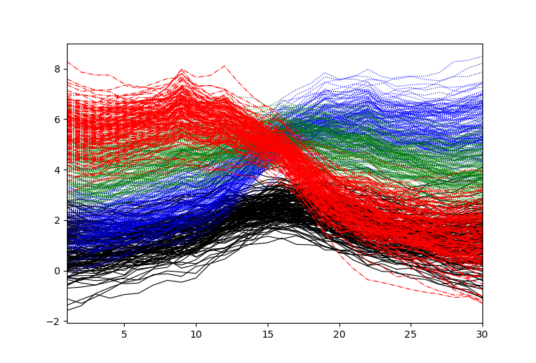
Refer to caption
Figure 2: Simulated Dataset 2. The true component memberships are indicated by colours and the estimated group memberships are indicated by line style: alternating dashes, small dots, and solid lines represent Groups 1, 2, and 3, respectively.

The EM algorithm is run for G=1,…,6G=1,\dots,6 components and q=5,…,9q=5,\dots,9 latent time points, again using multiple runs of both random starting values and kk-means clustering to initialize the z^i​g\hat{z}_{ig} values. The resulting BIC values are shown in Figure 3: two, three, or perhaps four groups, and seven time latent time points, appear to give the best fit for the data. The best model has G=3G=3 components and q=7q=7 latent time points, and the resulting clustering performance of this model is summarized in Table 3. The associated ARI is 0.69, indicating good clustering performance despite the “correct” number of components not being chosen. More specifically, we see from Table 3 that observations from components 1 and 4 are almost perfectly classified, while observations from components 2 and 3 are essentially classified into one group.

Refer to caption
Figure 3: BIC values versus the number of groups, where the numbers 5,…,95,\dots,9 indicate the number of latent time points.
Table 3: True group memberships (A–D) cross-tabulated against predicted group memberships (1–3) for the second simulated data set.
1 2 3
A 150 0 0
B 0 149 1
C 0 150 0
D 0 4 146

A total of 298 parameters are required for our fitted model. Without utilizing any latent factors, the (unconstrained) component covariance matrices alone would require G⁡[p⁡(p−1)/2]+G​p=465​GG[p(p-1)/2]+Gp=465G parameters. Thus, the model was able to achieve good clustering performance on this longitudinal data set using a significantly reduced number of parameters.

3.4 Yeast Sporulation Data Set

The final data set consists of 6,118 expressions of yeast genes measured at p=7p=7 time points, analyzed previously by various researchers to find groups of genes exhibiting similar expression patterns Mitchell (1994); Chu et al. (1998); Wakefield et al. (2003); McNicholas and Murphy (2010).

Refer to caption
Figure 4: BIC values versus the number of groups, where the numbers 3, 4, and 5 indicate the number of latent time points.
Refer to caption
Figure 5: BIC values versus the number of groups for q=5q=5 latent time points.
Refer to caption
Figure 6: Yeast gene expressions (after taking the negative logarithm, base 2, and standardizing) coloured by estimated group memberships, with estimated group mean trajectories (given by 𝚲^​𝝃^g\hat{\mathbf{\Lambda}}\hat{\bm{\xi}}_{g} for g=1,…,10g=1,\dots,10).

To test the performance of the proposed model, we follow the analysis of McNicholas and Murphy (2010) and consider all seven time points without the deletion of any genes, and take the negative logarithm, base 2, of each observation prior to analysis. The observations at each time point are also standardized to have mean 0 and variance 1. The model is then fitted for G=1,…,20G=1,\dots,20 components and q=3,4,5q=3,4,5 latent time points. The zi​gz_{ig} are again initialized using both random starting values and kk-means clustering. The resulting BIC values for each model are shown in Figure 4. The best model, as seen more clearly in Figure 5, has GG = 10 groups and qq = 5 latent time points. The resulting groups are pictured in Figure 6, and are compared to the groups found by McNicholas and Murphy (2010) in Table 4.

Table 4: Predicted group memberships (A–M) found by McNicholas and Murphy (2010) cross-tabulated against predicted group memberships found by the new model (1–10), for the yeast data set.
Predicted
1 2 3 4 5 6 7 8 9 10
A 15 0 0 0 0 0 85 15 7 28
B 7 23 0 0 13 0 439 131 175 160
C 56 2 0 57 325 0 54 31 5 9
D 640 0 0 77 120 0 460 196 765 11
E 41 0 0 0 0 0 8 0 188 0
F 3 0 1 21 3 89 1 10 1 0
G 0 97 4 0 0 0 0 1 0 2
H 0 5 60 0 2 0 22 10 0 165
I 1 23 17 0 1 0 91 10 25 107
J 20 15 11 41 30 47 14 13 7 11
K 94 10 0 326 12 26 11 138 16 8
L 50 0 0 63 3 8 6 3 13 0
M 0 127 18 0 0 0 3 49 0 10

From Table 4, it seems clear that the model introduced herein found different groups of gene expressions. The fitted model requires 226 parameters, while the model that does not utilize any latent factors would require 359 parameters.

4 Summary

A mixture model for clustering high-dimensional longitudinal data was introduced, which has the ability to account for the longitudinal nature of the data being clustered while also providing significant data reduction. This is achieved using an extension of the mixture of common factor analyzers model, whereby the variability in measurements taken at many time points can be explained using a smaller number of (latent) time points. A modified Cholesky decomposition is used on the latent covariance matrices to account for the relationship between measurements in the latent space. Constraints can be placed on these latent covariance matrices to further reduce the number of parameters; however, the mixture of common factor analyzers approach used in this model provides significant data reduction even without doing so.

The model was fit to two simulated data sets and one real data set, overall demonstrating good clustering performance using a significantly reduced number of parameters. Use of the model on the first simulated data set resulted in a perfect clustering result, and use of the model on the second simulated data set, which consisted of 30 time points, yielded good clustering performance using only seven latent time points. Use of the model on the yeast sporulation data set allowed clustering of gene expressions to be achieved using a reduced number of parameters.

Further work could include applications to (real) longitudinal data sets consisting of a large number of time points. As well, note that the model outlined here is only useful for clustering univariate longitudinal data—that is, data that contain only one measurement taken at each time point. Anderlucci and Viroli (2015) use a mixture of matrix variate normal distributions to cluster multivariate longitudinal data; thus, future work could involve extending the model introduced here to account for longitudinal data that contain multiple measurements taken at each time point. Further, this model may be extended to include non-Gaussian distributions; for example, Gallaugher and McNicholas (2017) detail clustering using mixtures of skewed matrix variate distributions.

Appendix A Derivations of parameter estimates

Differentiating QQ, given by (13), with respect to 𝝃g\bm{\xi}_{g}, 𝐓g\mathbf{T}_{g}, 𝐃g−1\mathbf{D}_{g}^{-1}, 𝚲\mathbf{\Lambda}, and 𝚿−1\mathbf{\Psi}^{-1}, respectively, gives the score functions

S1​(ϑs)=∂Q∂𝝃g\displaystyle S_{1}(\bm{\vartheta}_{s})=\frac{\partial Q}{\partial\bm{\xi}_{g}} =−12∑i=1nz^i​g∂∂𝝃gtr{𝐓g′𝐃g−1𝐓g𝔼[(𝐔i​g−𝝃g)(𝐔i​g−𝝃g)′∣𝐱i,zi​g=1]}\displaystyle=-\frac{1}{2}\sum_{i=1}^{n}\hat{z}_{ig}\frac{\partial}{\partial\bm{\xi}_{g}}\text{tr}\left\{\mathbf{T}_{g}^{{}^{\prime}}\mathbf{D}_{g}^{-1}\mathbf{T}_{g}\mathbb{E}[(\mathbf{U}_{ig}-\bm{\xi}_{g})(\mathbf{U}_{ig}-\bm{\xi}_{g})^{{}^{\prime}}\mid\mathbf{x}_{i},z_{ig}=1]\right\}
=12∑i=1nz^i​g[𝐓g′𝐃g−1𝐓g𝔼[𝐔i​g∣𝐱i,zi​g=1]+𝐓g′𝐃g−1𝐓g𝔼[𝐔i​g∣𝐱i,zi​g=1]\displaystyle=\frac{1}{2}\sum_{i=1}^{n}\hat{z}_{ig}\Big[\mathbf{T}_{g}^{{}^{\prime}}\mathbf{D}_{g}^{-1}\mathbf{T}_{g}\mathbb{E}[\mathbf{U}_{ig}\mid\mathbf{x}_{i},z_{ig}=1]+\mathbf{T}_{g}^{{}^{\prime}}\mathbf{D}_{g}^{-1}\mathbf{T}_{g}\mathbb{E}[\mathbf{U}_{ig}\mid\mathbf{x}_{i},z_{ig}=1]
−(𝐓g′𝐃g−1𝐓g+𝐓g′𝐃g−1𝐓g)𝝃g]\displaystyle\hskip 30.00005pt-(\mathbf{T}_{g}^{{}^{\prime}}\mathbf{D}_{g}^{-1}\mathbf{T}_{g}+\mathbf{T}_{g}^{{}^{\prime}}\mathbf{D}_{g}^{-1}\mathbf{T}_{g})\bm{\xi}_{g}\Big]
=𝐓g′𝐃g−1𝐓g∑i=1nz^i​g(𝔼[𝐔i​g∣𝐱i,zi​g=1]−𝝃g),\displaystyle=\mathbf{T}_{g}^{{}^{\prime}}\mathbf{D}_{g}^{-1}\mathbf{T}_{g}\sum_{i=1}^{n}\hat{z}_{ig}\left(\mathbb{E}[\mathbf{U}_{ig}\mid\mathbf{x}_{i},z_{ig}=1]-\bm{\xi}_{g}\right),
S2​(ϑs)=∂Q∂𝐓g\displaystyle S_{2}(\bm{\vartheta}_{s})=\frac{\partial Q}{\partial\mathbf{T}_{g}} =−12∑i=1nz^i​g∂∂𝐓gtr{𝐓g′𝐃g−1𝐓g𝔼[(𝐔i​g−𝝃g)(𝐔i​g−𝝃g)′∣𝐱i,zi​g=1]}\displaystyle=-\frac{1}{2}\sum_{i=1}^{n}\hat{z}_{ig}\frac{\partial}{\partial\mathbf{T}_{g}}\text{tr}\left\{\mathbf{T}_{g}^{{}^{\prime}}\mathbf{D}_{g}^{-1}\mathbf{T}_{g}\mathbb{E}[(\mathbf{U}_{ig}-\bm{\xi}_{g})(\mathbf{U}_{ig}-\bm{\xi}_{g})^{{}^{\prime}}\mid\mathbf{x}_{i},z_{ig}=1]\right\}
=−ng𝐃g−1𝐓g1ng∑i=1nz^i​g𝔼[(𝐔i​g−𝝃g)(𝐔i​g−𝝃g)′∣𝐱i,zi​g=1]\displaystyle=-n_{g}\mathbf{D}_{g}^{-1}\mathbf{T}_{g}\frac{1}{n_{g}}\sum_{i=1}^{n}\hat{z}_{ig}\mathbb{E}[(\mathbf{U}_{ig}-\bm{\xi}_{g})(\mathbf{U}_{ig}-\bm{\xi}_{g})^{{}^{\prime}}\mid\mathbf{x}_{i},z_{ig}=1]
=−ng​𝐃g−1​𝐓g​𝐒g,\displaystyle=-n_{g}\mathbf{D}_{g}^{-1}\mathbf{T}_{g}\mathbf{S}_{g},

where

𝐒g\displaystyle\mathbf{S}_{g} =1ng∑i=1nz^i​g𝔼[(𝐔i​g−𝝃g)(𝐔i​g−𝝃g)′∣𝐱i,zi​g=1]\displaystyle=\frac{1}{n_{g}}\sum_{i=1}^{n}\hat{z}_{ig}\mathbb{E}[(\mathbf{U}_{ig}-\bm{\xi}_{g})(\mathbf{U}_{ig}-\bm{\xi}_{g})^{{}^{\prime}}\mid\mathbf{x}_{i},z_{ig}=1]
=1ng∑i=1nz^i​g(𝕍ar[𝐔i​g−𝝃g∣𝐱i,zi​g=1]+𝔼[𝐔i​g−𝝃g∣𝐱i,zi​g=1]𝔼[(𝐔i​g−𝝃g)′∣𝐱i,zi​g=1])\displaystyle=\frac{1}{n_{g}}\sum_{i=1}^{n}\hat{z}_{ig}\left(\mathbb{V}\text{ar}[\mathbf{U}_{ig}-\bm{\xi}_{g}\mid\mathbf{x}_{i},z_{ig}=1]+\mathbb{E}[\mathbf{U}_{ig}-\bm{\xi}_{g}\mid\mathbf{x}_{i},z_{ig}=1]\mathbb{E}[(\mathbf{U}_{ig}-\bm{\xi}_{g})^{{}^{\prime}}\mid\mathbf{x}_{i},z_{ig}=1]\right)
=1ng∑i=1nz^i​g[(𝐈q−𝜷^g𝚲^)(𝐓^g′𝐃^g−1𝐓^g)−1+𝜷^g(𝐱i−𝚲^𝝃^g)(𝐱i−𝚲^𝝃^g)′𝜷^g′],\displaystyle=\frac{1}{n_{g}}\sum_{i=1}^{n}\hat{z}_{ig}\left[(\mathbf{I}_{q}-\hat{\mathbf{\mbox{\boldmath$\beta$}}}_{g}\hat{\mathbf{\Lambda}})(\hat{\mathbf{T}}_{g}^{{}^{\prime}}\hat{\mathbf{D}}_{g}^{-1}\hat{\mathbf{T}}_{g})^{-1}+\hat{\mathbf{\mbox{\boldmath$\beta$}}}_{g}(\mathbf{x}_{i}-\hat{\mathbf{\Lambda}}\hat{\bm{\xi}}_{g})(\mathbf{x}_{i}-\hat{\mathbf{\Lambda}}\hat{\bm{\xi}}_{g})^{{}^{\prime}}\hat{\mathbf{\mbox{\boldmath$\beta$}}}_{g}^{{}^{\prime}}\right],
S3​(ϑs)=∂Q∂𝐃g−1\displaystyle S_{3}(\bm{\vartheta}_{s})=\frac{\partial Q}{\partial\mathbf{D}_{g}^{-1}} =12∑i=1nz^i​g[1|𝐃g−1|∂∂𝐃g−1|𝐃g−1|\displaystyle=\frac{1}{2}\sum_{i=1}^{n}\hat{z}_{ig}\Bigg[\frac{1}{\left|\mathbf{D}_{g}^{-1}\right|}\frac{\partial}{\partial\mathbf{D}_{g}^{-1}}\left|\mathbf{D}_{g}^{-1}\right|
−∂∂𝐃g−1tr{𝐓g′𝐃g−1𝐓g𝔼[(𝐔i​g−𝝃g)(𝐔i​g−𝝃g)′∣𝐱i,zi​g=1]}]\displaystyle\hskip 30.00005pt-\frac{\partial}{\partial\mathbf{D}_{g}^{-1}}\text{tr}\left\{\mathbf{T}_{g}^{{}^{\prime}}\mathbf{D}_{g}^{-1}\mathbf{T}_{g}\mathbb{E}[(\mathbf{U}_{ig}-\bm{\xi}_{g})(\mathbf{U}_{ig}-\bm{\xi}_{g})^{{}^{\prime}}\mid\mathbf{x}_{i},z_{ig}=1]\right\}\Bigg]
=ng2𝐃g−12∑i=1nz^i​g𝐓g(𝕍ar[𝐔i​g−𝝃g∣𝐱i,zi​g=1]\displaystyle=\frac{n_{g}}{2}\mathbf{D}_{g}-\frac{1}{2}\sum_{i=1}^{n}\hat{z}_{ig}\mathbf{T}_{g}\Big(\mathbb{V}\text{ar}[\mathbf{U}_{ig}-\bm{\xi}_{g}\mid\mathbf{x}_{i},z_{ig}=1]
+𝔼[𝐔i​g−𝝃g∣𝐱i,zi​g=1]𝔼[(𝐔i​g−𝝃g)′∣𝐱i,zi​g=1])𝐓g′,\displaystyle\hskip 30.00005pt+\mathbb{E}[\mathbf{U}_{ig}-\bm{\xi}_{g}\mid\mathbf{x}_{i},z_{ig}=1]\mathbb{E}[(\mathbf{U}_{ig}-\bm{\xi}_{g})^{{}^{\prime}}\mid\mathbf{x}_{i},z_{ig}=1]\Big)\mathbf{T}_{g}^{{}^{\prime}},
S4​(ϑs)=∂Q∂𝚲\displaystyle S_{4}(\bm{\vartheta}_{s})=\frac{\partial Q}{\partial\mathbf{\Lambda}} =−12∑i=1n∑g=1Gz^i​g∂∂𝚲tr{𝚿−1𝔼[(𝐱i−𝚲𝐔i​g)(𝐱i−𝚲𝐔i​g)′∣𝐱i,zi​g=1]}\displaystyle=-\frac{1}{2}\sum_{i=1}^{n}\sum_{g=1}^{G}\hat{z}_{ig}\frac{\partial}{\partial\mathbf{\Lambda}}\text{tr}\left\{\mathbf{\Psi}^{-1}\mathbb{E}[(\mathbf{x}_{i}-\mathbf{\Lambda}\mathbf{U}_{ig})(\mathbf{x}_{i}-\mathbf{\Lambda}\mathbf{U}_{ig})^{{}^{\prime}}\mid\mathbf{x}_{i},z_{ig}=1]\right\}
=−12∑i=1n∑g=1Gz^i​g∂∂𝚲tr{𝚿−1(𝐱i𝐱i′−𝚲𝔼[𝐔i​g∣𝐱i,zi​g=1]𝐱i′−𝐱i𝔼[𝐔i​g′∣𝐱i,zi​g=1]𝚲′\displaystyle=-\frac{1}{2}\sum_{i=1}^{n}\sum_{g=1}^{G}\hat{z}_{ig}\frac{\partial}{\partial\mathbf{\Lambda}}\text{tr}\Big\{\mathbf{\Psi}^{-1}\Big(\mathbf{x}_{i}\mathbf{x}_{i}^{{}^{\prime}}-\mathbf{\Lambda}\mathbb{E}\left[\mathbf{U}_{ig}\mid\mathbf{x}_{i},z_{ig}=1\right]\mathbf{x}_{i}^{{}^{\prime}}-\mathbf{x}_{i}\mathbb{E}\left[\mathbf{U}_{ig}^{{}^{\prime}}\mid\mathbf{x}_{i},z_{ig}=1\right]\mathbf{\Lambda}^{{}^{\prime}}
+𝚲𝔼[𝐔i​g𝐔i​g′∣𝐱i,zi​g=1]𝚲′)}\displaystyle\hskip 30.00005pt+\mathbf{\Lambda}\mathbb{E}\left[\mathbf{U}_{ig}\mathbf{U}_{ig}^{{}^{\prime}}\mid\mathbf{x}_{i},z_{ig}=1\right]\mathbf{\Lambda}^{{}^{\prime}}\Big)\Big\}
=∑i=1n∑g=1Gz^i​g𝚿−1(𝐱i𝔼[𝐔i​g′∣𝐱i,zi​g=1]−𝚲𝔼[𝐔i​g𝐔i​g′∣𝐱i,zi​g=1]),\displaystyle=\sum_{i=1}^{n}\sum_{g=1}^{G}\hat{z}_{ig}\mathbf{\Psi}^{-1}\left(\mathbf{x}_{i}\mathbb{E}[\mathbf{U}_{ig}^{{}^{\prime}}\mid\mathbf{x}_{i},z_{ig}=1]-\mathbf{\Lambda}\mathbb{E}[\mathbf{U}_{ig}\mathbf{U}_{ig}^{{}^{\prime}}\mid\mathbf{x}_{i},z_{ig}=1]\right),
S5​(ϑs)=∂Q∂𝚿−1\displaystyle S_{5}(\bm{\vartheta}_{s})=\frac{\partial Q}{\partial\mathbf{\Psi}^{-1}} =12∑i=1n∑g=1Gz^i​g[1|𝚿−1|∂∂𝚿−1|𝚿−1|\displaystyle=\frac{1}{2}\sum_{i=1}^{n}\sum_{g=1}^{G}\hat{z}_{ig}\bigg[\frac{1}{\left|\mathbf{\Psi}^{-1}\right|}\frac{\partial}{\partial\mathbf{\Psi}^{-1}}\left|\mathbf{\Psi}^{-1}\right|
−∂∂𝚿−1tr{𝚿−1𝔼[(𝐱i−𝚲𝐔i​g)(𝐱i−𝚲𝐔i​g)′∣𝐱i,zi​g=1]}]\displaystyle\hskip 30.00005pt-\frac{\partial}{\partial\mathbf{\Psi}^{-1}}\text{tr}\left\{\mathbf{\Psi}^{-1}\mathbb{E}[(\mathbf{x}_{i}-\mathbf{\Lambda}\mathbf{U}_{ig})(\mathbf{x}_{i}-\mathbf{\Lambda}\mathbf{U}_{ig})^{{}^{\prime}}\mid\mathbf{x}_{i},z_{ig}=1]\right\}\bigg]
=12∑i=1n∑g=1Gz^i​g(𝚿−𝔼[(𝐱i−𝚲𝐔i​g)(𝐱i−𝚲𝐔i​g)′∣𝐱i,zi​g=1])\displaystyle=\frac{1}{2}\sum_{i=1}^{n}\sum_{g=1}^{G}\hat{z}_{ig}\left(\mathbf{\Psi}-\mathbb{E}[(\mathbf{x}_{i}-\mathbf{\Lambda}\mathbf{U}_{ig})(\mathbf{x}_{i}-\mathbf{\Lambda}\mathbf{U}_{ig})^{{}^{\prime}}\mid\mathbf{x}_{i},z_{ig}=1]\right)
=n2𝚿−12∑i=1n∑g=1Gz^i​g(𝐱i𝐱i′−𝚲𝔼[𝐔i​g∣𝐱i,zi​g=1]𝐱i′−𝐱i𝔼[𝐔i​g′∣𝐱i,zi​g=1]𝚲′\displaystyle=\frac{n}{2}\mathbf{\Psi}-\frac{1}{2}\sum_{i=1}^{n}\sum_{g=1}^{G}\hat{z}_{ig}\Big(\mathbf{x}_{i}\mathbf{x}_{i}^{{}^{\prime}}-\mathbf{\Lambda}\mathbb{E}[\mathbf{U}_{ig}\mid\mathbf{x}_{i},z_{ig}=1]\mathbf{x}_{i}^{{}^{\prime}}-\mathbf{x}_{i}\mathbb{E}[\mathbf{U}_{ig}^{{}^{\prime}}\mid\mathbf{x}_{i},z_{ig}=1]\mathbf{\Lambda}^{{}^{\prime}}
+𝚲𝔼[𝐔i​g𝐔i​g′∣𝐱i,zi​g=1]𝚲′).\displaystyle\hskip 30.00005pt+\mathbf{\Lambda}\mathbb{E}[\mathbf{U}_{ig}\mathbf{U}_{ig}^{{}^{\prime}}\mid\mathbf{x}_{i},z_{ig}=1]\mathbf{\Lambda}^{{}^{\prime}}\Big).

Solving S1​(𝝃^gnew,𝐓^gnew,𝐃^gnew,𝚲^new,𝚿^new)=𝟎S_{1}(\hat{\bm{\xi}}_{g}^{\text{new}},\hat{\mathbf{T}}_{g}^{\text{new}},\hat{\mathbf{D}}_{g}^{\text{new}},\hat{\mathbf{\Lambda}}^{\text{new}},\hat{\mathbf{\Psi}}^{\text{new}})=\bf{0} gives

𝐓^g′𝐃^g−1𝐓^g∑i=1nz^i​g(𝔼[𝐔i​g∣𝐱i,zi​g=1]−𝝃^gnew)=𝟎\displaystyle\hat{\mathbf{T}}_{g}^{{}^{\prime}}\hat{\mathbf{D}}_{g}^{-1}\hat{\mathbf{T}}_{g}\sum_{i=1}^{n}\hat{z}_{ig}\left(\mathbb{E}[\mathbf{U}_{ig}\mid\mathbf{x}_{i},z_{ig}=1]-\hat{\bm{\xi}}_{g}^{\text{new}}\right)=\bf{0}
⟹ng𝝃^gnew=∑i=1nz^i​g𝔼[𝐔i​g∣𝐱i,zi​g=1]\displaystyle\implies n_{g}\hat{\bm{\xi}}_{g}^{\text{new}}=\sum_{i=1}^{n}\hat{z}_{ig}\mathbb{E}[\mathbf{U}_{ig}\mid\mathbf{x}_{i},z_{ig}=1]
⟹𝝃^gnew=𝝃^g+1ng​∑i=1nz^i​g​𝜷^g​(𝐱i−𝚲^​𝝃^g).\displaystyle\implies\hat{\bm{\xi}}_{g}^{\text{new}}=\hat{\bm{\xi}}_{g}+\frac{1}{n_{g}}\sum_{i=1}^{n}\hat{z}_{ig}\hat{\mbox{\boldmath$\beta$}}_{g}(\mathbf{x}_{i}-\hat{\mathbf{\Lambda}}\hat{\bm{\xi}}_{g}).

Then, solving diag​{S3​(𝝃^gnew,𝐓^gnew,𝐃^gnew,𝚲^new,𝚿^new)}=𝟎\text{diag}\left\{S_{3}(\hat{\bm{\xi}}_{g}^{\text{new}},\hat{\mathbf{T}}_{g}^{\text{new}},\hat{\mathbf{D}}_{g}^{\text{new}},\hat{\mathbf{\Lambda}}^{\text{new}},\hat{\mathbf{\Psi}}^{\text{new}})\right\}=\bf{0},

ng2𝐃^gnew−12diag{∑i=1nz^i​g𝐓^g(𝕍ar[𝐔i​g−𝝃g∣𝐱i,zi​g=1]\displaystyle\frac{n_{g}}{2}\hat{\mathbf{D}}_{g}^{\text{new}}-\frac{1}{2}\text{diag}\Bigg\{\sum_{i=1}^{n}\hat{z}_{ig}\hat{\mathbf{T}}_{g}\Big(\mathbb{V}\text{ar}[\mathbf{U}_{ig}-\bm{\xi}_{g}\mid\mathbf{x}_{i},z_{ig}=1]
+𝔼[𝐔i​g−𝝃g∣𝐱i,zi​g=1]𝔼[(𝐔i​g−𝝃g)′∣𝐱i,zi​g=1])𝐓^g′}=𝟎\displaystyle\hskip 110.00017pt+\mathbb{E}[\mathbf{U}_{ig}-\bm{\xi}_{g}\mid\mathbf{x}_{i},z_{ig}=1]\mathbb{E}[(\mathbf{U}_{ig}-\bm{\xi}_{g})^{{}^{\prime}}\mid\mathbf{x}_{i},z_{ig}=1]\Big)\hat{\mathbf{T}}_{g}^{{}^{\prime}}\Bigg\}=\bf{0}
⟹𝐃^gnew=diag{𝐓^g(𝐈q−𝜷^g𝚲^)𝐓^g−1𝐃^g+1ng∑i=1nz^i​g𝐓^g𝜷^g(𝐱i−𝚲^𝝃^g)(𝐱i−𝚲^𝝃^g)′𝜷^g′𝐓^g′},\displaystyle\implies\hat{\mathbf{D}}_{g}^{\text{new}}=\text{diag}\left\{\hat{\mathbf{T}}_{g}(\mathbf{I}_{q}-\hat{\mathbf{\mbox{\boldmath$\beta$}}}_{g}\hat{\mathbf{\Lambda}})\hat{\mathbf{T}}_{g}^{-1}\hat{\mathbf{D}}_{g}+\frac{1}{n_{g}}\sum_{i=1}^{n}\hat{z}_{ig}\hat{\mathbf{T}}_{g}\hat{\mathbf{\mbox{\boldmath$\beta$}}}_{g}(\mathbf{x}_{i}-\hat{\mathbf{\Lambda}}\hat{\bm{\xi}}_{g})(\mathbf{x}_{i}-\hat{\mathbf{\Lambda}}\hat{\bm{\xi}}_{g})^{{}^{\prime}}\hat{\mathbf{\mbox{\boldmath$\beta$}}}_{g}^{{}^{\prime}}\hat{\mathbf{T}}_{g}^{{}^{\prime}}\right\},

and S4​(𝝃^gnew,𝐓^gnew,𝐃^gnew,𝚲^new,𝚿^new)=𝟎S_{4}(\hat{\bm{\xi}}_{g}^{\text{new}},\hat{\mathbf{T}}_{g}^{\text{new}},\hat{\mathbf{D}}_{g}^{\text{new}},\hat{\mathbf{\Lambda}}^{\text{new}},\hat{\mathbf{\Psi}}^{\text{new}})=\bf{0}

⟹∑i=1n∑g=1Gz^i​g𝚿−1(𝐱i𝔼[𝐔i​g′∣𝐱i,zi​g=1]−𝚲𝔼[𝐔i​g𝐔i​g′∣𝐱i,zi​g=1])=𝟎\displaystyle\implies\sum_{i=1}^{n}\sum_{g=1}^{G}\hat{z}_{ig}\mathbf{\Psi}^{-1}\left(\mathbf{x}_{i}\mathbb{E}[\mathbf{U}_{ig}^{{}^{\prime}}\mid\mathbf{x}_{i},z_{ig}=1]-\mathbf{\Lambda}\mathbb{E}[\mathbf{U}_{ig}\mathbf{U}_{ig}^{{}^{\prime}}\mid\mathbf{x}_{i},z_{ig}=1]\right)=\bf{0}
⟹𝚲^new={∑i=1n∑g=1Gz^i​g𝐱i[𝝃^g+𝜷^g(𝐱i−𝚲^𝝃^g)]′}{∑i=1n∑g=1Gz^i​g(𝐈q−𝜷^g𝚲^)(𝐓^g′𝐃^g−1𝐓^g)−1\displaystyle\implies\hat{\mathbf{\Lambda}}^{\text{new}}=\left\{\sum_{i=1}^{n}\sum_{g=1}^{G}\hat{z}_{ig}\mathbf{x}_{i}\left[\hat{\bm{\xi}}_{g}+\hat{\mbox{\boldmath$\beta$}}_{g}(\mathbf{x}_{i}-\hat{\mathbf{\Lambda}}\hat{\bm{\xi}}_{g})\right]^{{}^{\prime}}\right\}\Bigg\{\sum_{i=1}^{n}\sum_{g=1}^{G}\hat{z}_{ig}(\mathbf{I}_{q}-\hat{\mbox{\boldmath$\beta$}}_{g}\hat{\mathbf{\Lambda}})(\hat{\mathbf{T}}_{g}^{{}^{\prime}}\hat{\mathbf{D}}_{g}^{-1}\hat{\mathbf{T}}_{g})^{-1}
+∑i=1n∑g=1Gz^i​g[𝝃^g+𝜷^g(𝐱i−𝚲^𝝃^g)][𝝃^g+𝜷^g(𝐱i−𝚲^𝝃^g)]′}−1.\displaystyle\hskip 100.00015pt+\sum_{i=1}^{n}\sum_{g=1}^{G}\hat{z}_{ig}[\hat{\bm{\xi}}_{g}+\hat{\mathbf{\mbox{\boldmath$\beta$}}}_{g}(\mathbf{x}_{i}-\hat{\mathbf{\Lambda}}\hat{\bm{\xi}}_{g})][\hat{\bm{\xi}}_{g}+\hat{\mathbf{\mbox{\boldmath$\beta$}}}_{g}(\mathbf{x}_{i}-\hat{\mathbf{\Lambda}}\hat{\bm{\xi}}_{g})]^{{}^{\prime}}\Bigg\}^{-1}.

Finally, diag​{S5​(𝝃^gnew,𝐓^gnew,𝐃^gnew,𝚲^new,𝚿^new)}=𝟎\text{diag}\Big\{S_{5}(\hat{\bm{\xi}}_{g}^{\text{new}},\hat{\mathbf{T}}_{g}^{\text{new}},\hat{\mathbf{D}}_{g}^{\text{new}},\hat{\mathbf{\Lambda}}^{\text{new}},\hat{\mathbf{\Psi}}^{\text{new}})\Big\}=\bf{0}

⟹n2𝚿new−12diag{∑i=1n∑g=1Gz^i​g(𝐱i𝐱i′−𝚲𝔼[𝐔i​g∣𝐱i,zi​g=1]𝐱i′−𝐱i𝔼[𝐔i​g′∣𝐱i,zi​g=1]𝚲′\displaystyle\implies\frac{n}{2}\mathbf{\Psi}^{\text{new}}-\frac{1}{2}\text{diag}\Bigg\{\sum_{i=1}^{n}\sum_{g=1}^{G}\hat{z}_{ig}\Big(\mathbf{x}_{i}\mathbf{x}_{i}^{{}^{\prime}}-\mathbf{\Lambda}\mathbb{E}[\mathbf{U}_{ig}\mid\mathbf{x}_{i},z_{ig}=1]\mathbf{x}_{i}^{{}^{\prime}}-\mathbf{x}_{i}\mathbb{E}[\mathbf{U}_{ig}^{{}^{\prime}}\mid\mathbf{x}_{i},z_{ig}=1]\mathbf{\Lambda}^{{}^{\prime}}
+𝚲𝔼[𝐔i​g𝐔i​g′∣𝐱i,zi​g=1]𝚲′)}=𝟎\displaystyle\hskip 100.00015pt+\mathbf{\Lambda}\mathbb{E}[\mathbf{U}_{ig}\mathbf{U}_{ig}^{{}^{\prime}}\mid\mathbf{x}_{i},z_{ig}=1]\mathbf{\Lambda}^{{}^{\prime}}\Big)\Bigg\}=\bf{0}
⟹𝚿^new=1ndiag{∑i=1n∑g=1Gz^i​g(𝐱i𝐱i′−𝚲^𝔼[𝐔i​g∣𝐱i,zi​g=1]𝐱i′−𝐱i𝔼[𝐔i​g′∣𝐱i,zi​g=1]𝚲^′\displaystyle\implies\hat{\mathbf{\Psi}}^{\text{new}}=\frac{1}{n}\text{diag}\Bigg\{\sum_{i=1}^{n}\sum_{g=1}^{G}\hat{z}_{ig}\Big(\mathbf{x}_{i}\mathbf{x}_{i}^{{}^{\prime}}-\hat{\mathbf{\Lambda}}\mathbb{E}[\mathbf{U}_{ig}\mid\mathbf{x}_{i},z_{ig}=1]\mathbf{x}_{i}^{{}^{\prime}}-\mathbf{x}_{i}\mathbb{E}[\mathbf{U}_{ig}^{{}^{\prime}}\mid\mathbf{x}_{i},z_{ig}=1]\hat{\mathbf{\Lambda}}^{{}^{\prime}}
+𝚲^𝔼[𝐔i​g𝐔i​g′∣𝐱i,zi​g=1]𝚲^′)}\displaystyle\hskip 100.00015pt+\hat{\mathbf{\Lambda}}\mathbb{E}[\mathbf{U}_{ig}\mathbf{U}_{ig}^{{}^{\prime}}\mid\mathbf{x}_{i},z_{ig}=1]\hat{\mathbf{\Lambda}}^{{}^{\prime}}\Big)\Bigg\}
⟹𝚿^new=1ndiag{∑i=1n∑g=1Gz^i​g(𝐱i𝐱i′−𝚲^[𝝃^g+𝜷^g(𝐱i−𝚲^𝝃^g)]𝐱i′\displaystyle\implies\hat{\mathbf{\Psi}}^{\text{new}}=\frac{1}{n}\text{diag}\Bigg\{\sum_{i=1}^{n}\sum_{g=1}^{G}\hat{z}_{ig}\bigg(\mathbf{x}_{i}\mathbf{x}_{i}^{{}^{\prime}}-\hat{\mathbf{\Lambda}}\left[\hat{\bm{\xi}}_{g}+\hat{\mbox{\boldmath$\beta$}}_{g}(\mathbf{x}_{i}-\hat{\mathbf{\Lambda}}\hat{\bm{\xi}}_{g})\right]\mathbf{x}_{i}^{{}^{\prime}}
−𝐱i[𝝃^g+𝜷^g(𝐱i−𝚲^𝝃^g)]′𝚲^′+𝚲^[(𝐈q−𝜷^g𝚲^)(𝐓^g′𝐃^g−1𝐓^g)−1\displaystyle\hskip 100.00015pt-\mathbf{x}_{i}\left[\hat{\bm{\xi}}_{g}+\hat{\mbox{\boldmath$\beta$}}_{g}(\mathbf{x}_{i}-\hat{\mathbf{\Lambda}}\hat{\bm{\xi}}_{g})\right]^{{}^{\prime}}\hat{\mathbf{\Lambda}}^{{}^{\prime}}+\hat{\mathbf{\Lambda}}\bigg[(\mathbf{I}_{q}-\hat{\mbox{\boldmath$\beta$}}_{g}\hat{\mathbf{\Lambda}})(\hat{\mathbf{T}}_{g}^{{}^{\prime}}\hat{\mathbf{D}}_{g}^{-1}\hat{\mathbf{T}}_{g})^{-1}
+[𝝃^g+𝜷^g(𝐱i−𝚲^𝝃^g)][𝝃^g+𝜷^g(𝐱i−𝚲^𝝃^g)]′]𝚲^′)}.\displaystyle\hskip 100.00015pt+\Big[\hat{\bm{\xi}}_{g}+\hat{\mbox{\boldmath$\beta$}}_{g}(\mathbf{x}_{i}-\hat{\mathbf{\Lambda}}\hat{\bm{\xi}}_{g})\Big]\Big[\hat{\bm{\xi}}_{g}+\hat{\mbox{\boldmath$\beta$}}_{g}(\mathbf{x}_{i}-\hat{\mathbf{\Lambda}}\hat{\bm{\xi}}_{g})\Big]^{{}^{\prime}}\bigg]\hat{\mathbf{\Lambda}}^{{}^{\prime}}\bigg)\Bigg\}.

References

  • Aitken (1926) Aitken, A. C. (1926). A series formula for the roots of algebraic and transcendental equations. Proceedings of the Royal Society of Edinburgh 45, 14–22.
  • Anderlucci and Viroli (2015) Anderlucci, L. and C. Viroli (2015). Covariance pattern mixture models for multivariate longitudinal data. The Annals of Applied Statistics 9(2), 777–800.
  • Baek et al. (2010) Baek, J., G. J. McLachlan, and L. K. Flack (2010). Mixtures of factor analyzers with common factor loadings: Applications to the clustering and visualization of high-dimensional data. IEEE Transactions on Pattern Analysis and Machine Intelligence 32, 1298–1309.
  • Böhning et al. (1994) Böhning, D., E. Dietz, R. Schaub, P. Schlattmann, and B. Lindsay (1994). The distribution of the likelihood ratio for mixtures of densities from the one-parameter exponential family. Annals of the Institute of Statistical Mathematics 46, 373–388.
  • Cheam et al. (2017) Cheam, A. S. M., M. Marbac, and P. D. McNicholas (2017). Model-based clustering for spatiotemporal data on air quality monitoring. Environmetrics 93, 192–206.
  • Chu et al. (1998) Chu, S., J. DeRisi, M. Eisen, J. Mulholland, D. Botstein, P. O. Brown, and I. Herskowitz (1998). The transcriptional program of sporulation in budding yeast. Science 282(5389), 699–705.
  • Dasgupta and Raftery (1998) Dasgupta, A. and A. E. Raftery (1998). Detecting features in spatial point processes with clutter via model-based clustering. Journal of the American Statistical Association 93, 294–302.
  • Dempster et al. (1977) Dempster, A. P., N. M. Laird, and D. B. Rubin (1977). Maximum likelihood from incomplete data via the EM algorithm. Journal of the Royal Statistical Society: Series B 39(1), 1–38.
  • Gallaugher and McNicholas (2017) Gallaugher, M. P. and P. D. McNicholas (2017). A mixture of matrix variate skew-t distributions. arXiv preprint arXiv:1703.08882.
  • Ghahramani and Hinton (1997) Ghahramani, Z. and G. E. Hinton (1997). The EM algorithm for factor analyzers. Technical Report CRG-TR-96-1, University of Toronto, Toronto, Canada.
  • Han et al. (2017) Han, S., H. Zhang, W. Karmaus, G. Roberts, and H. Arshad (2017). Adjusting background noise in cluster analyses of longitudinal data. Computational Statistics & Data Analysis 109, 93–104.
  • Hubert and Arabie (1985) Hubert, L. and P. Arabie (1985). Comparing partitions. Journal of Classification 2(1), 193–218.
  • Lütkepohl (1996) Lütkepohl, H. (1996). Handbook of Matrices. Chicester: John Wiley & Sons.
  • McLachlan and Peel (2000a) McLachlan, G. J. and D. Peel (2000a). Finite Mixture Models. New York: John Wiley & Sons.
  • McLachlan and Peel (2000b) McLachlan, G. J. and D. Peel (2000b). Mixtures of factor analyzers. In Proceedings of the Seventh International Conference on Machine Learning, San Francisco, pp. 599–606. Morgan Kaufmann.
  • McNicholas (2016) McNicholas, P. D. (2016). Mixture Model-Based Classification. Boca Raton: Chapman & Hall/CRC Press.
  • McNicholas and Murphy (2010) McNicholas, P. D. and T. B. Murphy (2010). Model-based clustering of longitudinal data. The Canadian Journal of Statistics 38(1), 153–168.
  • McNicholas et al. (2010) McNicholas, P. D., T. B. Murphy, A. F. McDaid, and D. Frost (2010). Serial and parallel implementations of model-based clustering via parsimonious Gaussian mixture models. Computational Statistics and Data Analysis 54(3), 711–723.
  • Melnykov (2016) Melnykov, V. (2016). Model-based biclustering of clickstream data. Computational Statistics and Data Analysis 93, 31–45.
  • Mitchell (1994) Mitchell, A. P. (1994). Control of meiotic gene expression in saccharomyces cerevisiae. Microbiological reviews 58(1), 56–70.
  • Pourahmadi (1999) Pourahmadi, M. (1999). Joint mean-covariance models with applications to longitudinal data: unconstrained parameterisation. Biometrika 86(3), 677–690.
  • Pourahmadi (2000) Pourahmadi, M. (2000). Maximum likelihood estimation of generalised linear models for multivariate normal covariance matrix. Biometrika 87(2), 425–435.
  • Rand (1971) Rand, W. M. (1971). Objective criteria for the evaluation of clustering methods. Journal of the American Statistical Association 66(336), 846–850.
  • Schwarz (1978) Schwarz, G. (1978). Estimating the dimension of a model. The Annals of Statistics 6(2), 461–464.
  • Wakefield et al. (2003) Wakefield, J., C. Zhou, and S. Self (2003). Modelling gene expression over time: curve clustering with informative prior distributions. Bayesian statistics 7, 721–732.
  • Yoshida et al. (2004) Yoshida, R., T. Higuchi, and S. Imoto (2004). A mixed factors model for dimension reduction and extraction of a group structure in gene expression data. In Proceedings of the 2004 IEEE Computational Systems Bioinformatics Conference, pp. 161–172.
  • Yoshida et al. (2006) Yoshida, R., T. Higuchi, S. Imoto, and S. Miyano (2006). ArrayCluster: an analytic tool for clustering, data visualization and module finder on gene expression profiles. Bioinformatics 22, 1538–1539.