Multi-Sound-Source Localization Using Machine Learning for Small Autonomous Unmanned Vehicles with a Self-Rotating Bi-Microphone Array
Abstract
While vision-based localization techniques have been widely studied for small autonomous unmanned vehicles (SAUVs), sound-source localization capabilities have not been fully enabled for SAUVs. This paper presents two novel approaches for SAUVs to perform three-dimensional (3D) multi-sound-sources localization (MSSL) using only the inter-channel time difference (ICTD) signal generated by a self-rotating bi-microphone array. The proposed two approaches are based on two machine learning techniques viz., Density-Based Spatial Clustering of Applications with Noise (DBSCAN) and Random Sample Consensus (RANSAC) algorithms, respectively, whose performances are tested and compared in both simulations and experiments. The results show that both approaches are capable of correctly identifying the number of sound sources along with their 3D orientations in a reverberant environment.
1 Introduction
Small autonomous unmanned vehicles (SAUVs, e.g., quadcopters and ground robots) have revolutionized civilian and military missions by creating a platform for observation and permitting access to locations that are too dangerous, too difficult or too costly to send humans. The sensing capability of SAUVs has been enabled by various sensors, such as RGB cameras, infrared cameras, LiDARs, RADARs, and ultrasound sensors. However, these mainstream sensors are subject to either lighting conditions or line-of-sight requirements. On the other end of the spectrum, as the sound travels to all directions and can be transmitted even with some small obstacles [1], sound sensors have great potential to overcome the line-of-sight constraints of the aforementioned sensors and provide SAUVs with an omnidirectional full span sensing coverage. Sound-based sensing capabilities would significantly facilitate SAUVs in critical applications (e.g., search and rescue) and enable sociable and service robots (e.g., shopping assistants and restaurant waiters) to collaborate with humans in complicated scenarios [2, 3].
Among the sensing tasks for SAUVs, localization is of utmost significance [4]. While vision-based localization techniques have been developed based on cameras, sound source localization (SSL) has been achieved using microphone arrays with different numbers (e.g., 2, 4, 8, 16) of microphones. Although it has been reported that the accuracy of the localization is enhanced as the number of microphones increases [5, 6], this comes with a price of algorithm complexity and hardware cost, especially due to the expense of Analog-to-Digital converters (ADC), which is proportional to the number of speaker channels.
Humans and many other animals can locate sound sources with decent accuracy and responsiveness by using their two ears associated with head rotations to avoid ambiguity (i.e., cone of confusion) [7]. SSL techniques using a self-rotating bi-microphone array have been reported in the literature [8, 9, 10, 11, 12]. To eliminate cone of confusion [7], the bi-microphone array is rotated around the center of the robot/dummy head on the horizontal plane so that an Inter-Channel Time Difference (ICTD) signal is generated whose data points form multiple discontinuous sinusoidal waveforms. Single-SSL (SSSL) techniques with different numbers of microphones have been well-studied [13], while reported multi-sound-source-localization (MSSL) techniques typically require large microphone arrays with specific structures, which are not easy to be mounted on SAUVs. Pioneer work for MSSL assumed the number of sources to be known beforehand [14, 15]. Some of these approaches [16, 17, 18] are based on sparse component analysis (SCA) that requires the sources to be W-disjoint orthogonal [19] (i.e., in some time-frequency components, at most one source is active), thereby making them unsuitable for reverberant environments. Pavlidi et al. [20] and Loesch et al. [21] presented an SCA-based method that counts and localizes multiple sound sources but requires one sound source to be dominant over others in a time-frequency zone.
Clustering methods have also been used to conduct MSSL [17, 16, 18]. Catalbas et al. [22] presented an approach for MSSL by using four microphones and the sound sources are required to be present within a predefined boundary. The technique was limited to localize sound orientations in the two-dimensional plane using k-medoids clustering. The number of sound sources was calculated using the exhaustive elbow method, which is instinctive and computationally expensive. Traa et al. [23] presented an approach that utilizes the time-delay between the microphones in the frequency domain to model the phase differences in each frequency bin of a short-time Fourier transform. Using the linear relationship between phase difference and frequency, the data were then clustered using random sample consensus (RANSAC). In our previous work [12, 11, 24, 25], we developed an SSSL technique based on an extended Kalman filter and an MSSL technique based on a cross-correlation approach, which was computationally expensive.
The contributions of this paper include two novel MSSL approaches for SAUVs. Both approaches are able to identify both the number of sound sources and their 3D locations by only using a self-rotating bi-microphone array. In the first approach, a novel mapping mechanism is developed to convert the acquired ICTD signal to an orientation domain. Unsupervised classification is then conducted using the Density-Based Spatial Clustering of Applications with Noise (DBSCAN) [26]. The second approach is based on a sinusoidal ICTD regression using a RANSAC-based method. Both simulations and experiments were conducted to verify the proposed methodology.
The rest of the paper is organized as follows. In Section 2, the mathematical calculation for the ICTD signal generated by the self-rotating microphone array is presented. In Section 3, the mapping mechanism for regression and clustering is presented. Section 4 presents the two proposed approaches for MSSL. Simulation and experimental results are presented and discussed in Section 5. Section 6 concludes the paper.
2 Preliminaries
2.1 Inter-Channel Time Difference (ICTD)
The ICTD is the time difference between a sound signal arriving at two microphones and can be calculated using the cross-correlation technique [27, 28]. Consider a single stationary sound source and two spatially separated microphones placed in an environment. Let and be the sound signals captured by the microphones in presence of noise, which are given by [27] and , where is the sound signal, and are real and jointly stationary random noises, denotes the time difference of arriving at the two microphones, and is the signal attenuation factor due to different traveling distances. It is commonly assumed that changes slowly and is uncorrelated with noises and [27].
The cross-correlation of and is given by , where represents the expectation operator. Various pre-filters that eliminate or reduce the effect of background noise and reverberations have been used prior to the cross-correlation [29, 30, 31]. The time difference of and , i.e., the ICTD, is given by The distance difference of the sound signal traveling to the two microphones is given by where is the sound speed and is usually selected as 345 m/s on the Earth surface.
Remark 1
For simplicity, the signal is referred as ICTD in this paper. ICTD is the only cue used in this paper for the source counting and localization, while no aforementioned scaling functions nor pre-filters are used.
2.2 Far-Field Assumption
The five different fields around a sound source are free field, near field, far field, direct field, and reverberant field [32, 33]. The region where the sound pressure and the acoustic particle velocity are not in phase is regarded as the near field. The far field of a source begins where the near field ends and extends to infinity. Under the far-field assumption, the acoustic wavefront reaching the microphones is planar and not spherical, in the sense that the waves travel in parallel. This means that the angle of incidence will be the same for the two microphones. Further, it can be shown that with , the error of the far-field approximation drops below , where is the distance of the sound source to the center of the microphone array and is the distance between the microphones [34].
2.3 Mathematical Model for ICTD signal
In this paper, the location of a single sound source is defined in a spherical coordinate frame, whose origin is assumed to coincide with the center of a ground robot.


As shown in Figs. 1 and 2, the left and right microphones, and , collects the acoustic signal generated by the sound source S. Let be the center of the robot as well as the bi-microphone array. The sound source location is represented by (), where is the distance between the source and the center of the robot, i.e., the length of segment , is the elevation angle defined as the angle between and the horizontal plane, and ] is the azimuth angle defined as the angle measured clockwise from the robot heading vector, , to . Letting unit vector be the orientation (heading) of the microphone array, be the angle from to , and be the angle from to , both following a clockwise rotation rule, we have
| (1) |
In the shaded triangle, , shown in Figs. 2 and 3, define and we have Based on the far-field assumption [32], we have
| (2) |
To avoid cone of confusion [7] in SSL, we are considering an ICTD signal generated by a microphone pair with time-varying positions, such as a self-rotating bi-microphone array. Without loss of generality, in this paper, we assume a clockwise rotation of the microphone array on the horizontal plane, while the robot itself does not rotate throughout the entire estimation process, which implies that in Equation (1) is constant. The rotation of the microphone array is assumed to be triggered by a sound detection mechanism, which is beyond the scope of this paper and hence will not be discussed.
The initial heading of the microphone array is configured to coincide with the heading of the robot, i.e., , which implies that . As the microphone array rotates clockwise with a constant angular velocity, , we have and due to Equation (1) we have The resulting time-varying due to Equation (2) is then given by
| (3) |
Because the microphone array rotates on the horizontal plane, does not change during the rotation for a stationary sound source. The resulting is a sinusoidal signal with the amplitude , which implies that
| (4) |
It can be seen from Equation (3) that the phase angle of is the azimuth angle of the sound source. Therefore, the location (i.e., azimuth and elevation angle) of the sound source can by determined by estimating the characteristics (i.e., the amplitude and phase angle) of the sinusoidal signal, .
The collection of the ICTD signal for multiple sound sources (as shown in Fig. 13a) illustrates a group of multiple discontinuous sinusoidal waveforms, each of which corresponds to a single sound source, satisfying the amplitude-elevation and phase-azimuth relationship as mentioned above.
3 Model for Mapping and Sinusoidal Regression
The signal in Equation (3) is sinusoidal with its amplitude and phase angle that corresponds to the azimuth angle of the sound source. Since the frequency, , of is the known rotational speed of the microphone array, the localization task (i.e., identifying and ) is to estimate the amplitude and phase angle of , i.e., and .
Consider a general form of expressed as
| (5) |
where and , and we have and Consider two data points and , collected at two distinct time instants and , respectively, and we have
| (6) |
If then we can obtain
| (7) |
and
| (8) |
4 Methodology
4.1 DBSCAN-Based MSSL
DBSCAN is one of the most popular nonlinear clustering techniques and it can discover any arbitrarily shaped clusters of densely grouped points in a data set and outperform other clustering methods in the literature [35, 36]. In the DBSCAN algorithm [35], a random point from the data set is considered as a core cluster point when more than points (including itself) within a distance of (epsilon ball) exists in its neighborhood. This cluster is then extended by checking all of the other points satisfying the criteria thereby letting the cluster grow. A new arbitrary point is then chosen and the process is repeated. The point which is not a part of any cluster and having fewer than points in its -ball is considered as a “noise point”. The DBSCAN technique is more suitable for applications with noise and outperforms the -means method, which requires a prior knowledge of the number and the approximate initial centroids of clusters and is highly sensitive to noisy data points and to the selection of the initial centroids [37].
The proposed DBSCAN-based MSSL technique consists of two stages. In the first stage, the data points of the ICTD signal are mapped to the orientation (i.e., the elevation-azimuth coordinate) domain. The data set consisting of all data points in a multi-source ICTD signal contains not only inliers but also outliers, which produce undesired mapped locations. When the number of inliers is significantly greater than the outliers after a number of iterations, highly dense clusters will be formed. In the second stage, these clusters are detected using the DBSCAN technique by carefully selecting parameters and . The number of clusters corresponds to the number of sound sources and the centroids of these clusters represent the locations of the sound sources.
The complete DBSCAN-based MSSL algorithm is described in Algorithm 1. Two points in the data set are selected randomly and mapped into the orientation domain by calculating angles and using Equations (3), (7), (4) and (8). A set of these mapped points is then created. The process for detection of clusters is then started. A point in is randomly chosen and is decided to be a core cluster point or a noise point by checking the density-reachability criteria under the - condition [35]. The time complexity of Algorithm 1 is , where is the number of iterations for mapping and clustering. The selection of parameters for Algorithm 1 will be discussed in Section 4.3.
1: Capture for one full rotation of the bi-microphone array
2: Select and
3: Select the number of iterations
4: FOR to DO
5: Randomly choose non-repeated set of two points and from , such that and do not equal zero simultaneously
7: Calculate using Equation (4) and
8: END FOR
9: FOR to DO
10: Randomly choose the pair from the set
11: Calculate the distance between the chosen and every other point in
12: IF the number of points in the range is greater than
13: Label as a core cluster point
14: ELSE
15: Label as a noise point
16: END IF
17: END FOR
4.2 RANSAC-Based MSSL
The RANSAC [38] algorithm iteratively uses a set of observed data to estimate parameters of a mathematical model and can identify inliers (e.g., parameters of a mathematical model) in a data set that may contain a significantly large number of outliers. The input to the RANSAC algorithm includes a set of data, a parameterized model, and a confidence parameter (). In each iteration, a subset of the original data is randomly selected and used to fit the predefined parameterized model. All other data points in the original data set are then tested against the fitted model. A point is determined to be an inlier of the fitted model, if it satisfies the condition. The process is repeated by selecting another random subset of the data. After a number of iterations, the parameters are then selected for the best fitting (with maximum inliers) estimated model.
1: Capture for one full rotation of the bi-microphone array
2: Select , and initialize
3: WHILE there are samples in
4: FOR to DO
5: Randomly choose non-repeated set of two points and from , such that and do not equal zero simultaneously
7: Calculate
8: Calculate = number of points in fitting with at least
9: IF
10: , and
11: END IF
12: END FOR
13: Calculate using Equation (4)
14:
15: Remove samples on within from
16: END WHILE
The RANSAC-based MSSL method is described in Algorithm 2. It can be seen from Equation (3) that the signal generated by the self-rotating bi-microphone array is sinusoidal. Two points from the ICTD signal are selected randomly and a sine wave with the given frequency (i.e., the angular speed of the rotation, is generated. The represents the number of points whose distance to the fitted sine wave is less than , which is the threshold for a point to be considered inlier. Then the points in that belong to according to the condition will be removed from , This procedure is repeated for iterations and the parameters and are updated every time the number of inliers is greater than that in the previous iterations. This process is repeated until either all the points in are examined or iterations are completed. The time complexity of Algorithm 2 is , where is the number of samples in the ICTD. After the first few of iterations, most of the data points are removed. This results in to be a small number as compared to .
4.3 Parameter Selection
The value of can be chosen depending on the possibility of sound sources to be close to each other and the noise level. The maximum number of possible unique combinations of randomly chosen data points and is , where the value of is the number of data points and is the number of randomly chosen data points. However, the number of iterations, , needs only to be large enough for the efficient formation of the clusters. The larger the value of , the denser the clusters would be, which will further modify the value in Algorithm 1. On the other hand, should be chosen large enough to ensure that at least one of the sets of randomly selected points does not include an outlier. The value of the can be smaller than due to the removal of all the data points within the range, which reduces the data points to further deal with. Further, these values also depends on how noisy the data is. The number of iterations for RANSAC-based MSSL can be calculated using , where is the probability of success, is outlier ratio and is the number of required points to fit the model.
The number of sound sources is determined by carefully selecting a threshold, as shown in Fig. 4. The confidence about the presence of a sound source is dependent on the value. The source with the maximum is considered to be qualified with 100 % confidence and the confidence values for other sources are calculated relatively. The source with a confidence value less than the threshold is considered to be noise and is not qualified as a sound source.

5 Simulation and Experimental Results
5.1 Simulation and Experimental Setup
Audio Array Toolbox [39] is used to establish an emulated rectangular room using the image method described in [40]. The robot was placed in the origin of the room. The sound sources and the microphones are assumed omnidirectional and the attenuation of the sound are calculated per the specifications in Table 1. Fig. 5 shows the simulation setup with the robot placed at the origin and the four sound sources placed at different azimuth and elevation angles.
| Parameter | Value |
|---|---|
| Dimension | 20 m x 20 m x 20 m |
| Reflection coefficient | 0.5 |
| (walls, floor and ceiling) | |
| Sound speed | 345 m/s |
| Temperature | 22 |
| Static pressure | 29.92 mmHg |
| Relative humidity | 38 % |

A number of recorded audio signals available at [41] were used as sound sources to test the technique. Different numbers of sound sources were placed at various azimuth and elevation angles at a fixed distance of and the ICTD signal was recorded by the rotating bi-microphone array with mics separated by a distance of m. The sound sources were separated by at least in azimuth and at least in elevation. The ICTD value was calculated and recorded every of rotation. Zero-mean noise with a variance ( of was added to this ICTD signal in simulations to account for sensor noise.


Experiments were conducted using a Kobuki Turtlebot 2 robot shown in Fig. 6 mounted with a robotic platform as shown in Fig. 7 consisting of two microelectromechanical systems (MEMS) analog microphones shown in Fig. 8. These experiments were conducted in an indoor environment with the reverberation time ms (where RT60 is the time required for a sound to decay 60 dB). Fig. 10 shows the impulse response of the room. The experimental setup is shown in Fig. 9. The sampling frequency of the two microphones was 44,100 Hz while recording the signal. A microphone evaluation board assembly was used for data acquisition. The angular speed of the rotation of the microphone array was controlled by a bipolar stepper motor with gear ratio adjusted to per step and rotating at an angular velocity of rad/sec which was controlled by an Arduino board. The distance between the two microphones was kept constant as m. Audio clips were played in a number of loudspeakers which were used as sound sources. These speakers were kept at different locations with a m distance from the robot, thereby satisfying the far-field approximation [34].

| Parameters | For simulations | For experiments |
|---|---|---|
| m | m | |
| Threshold | % | % |
| m | – |
5.2 Results and Discussion


Figures 11a and 11b show the formation of the clusters in simulation and real environment, respectively, during the mapping of ICTD data points to their respective and angles using Equations 4, 7 and 8.


Figures 12a and 12b show the detection of these clusters in simulation and real environment, respectively, using the DBSCAN technique for a sample run.
| Number | MAE (Sim) | MAE (Expt) | ||
|---|---|---|---|---|
| of | (deg) | (deg) | (deg) | (deg) |
| source(s) | DBSCAN | |||
| 4 | 1.73 | 3.20 | 3.71 | 5.66 |
| 3 | 0.8 | 4.68 | 1.77 | 5.78 |
| 2 | 1.06 | 2.18 | 2.89 | 3.92 |
| 1 | 0.94 | 0.57 | 2.27 | 0.35 |
| RANSAC | ||||
| 4 | 0.88 | 8.12 | 3.92 | 7.20 |
| 3 | 2.51 | 5.56 | 2.33 | 5.62 |
| 2 | 2.55 | 5.01 | 3.07 | 3.88 |
| 1 | 1.61 | 1.97 | 2.15 | 3.07 |
The parameters used for the RANSAC- and DBSCAN-based algorithms are listed in Table 2. The value was chosen to be m for simulation and m for experiments, which implies that the sound sources with the same azimuth are assumed to be separated by at least in elevation. Table 3 shows the simulation and experimental results of localization with the number of sound sources varying from one to four.
Monte Carlo simulation runs were performed using the two proposed approaches, respectively, with specifications given in Table 1. Simulations were run with sources and the results of the source counting are listed in the Table 4.
| Act | K | 1 | 2 | 3 | 4 | 5 | 6 | 7 |
|---|---|---|---|---|---|---|---|---|
| Estimated - DBSCAN | ||||||||
| 1 | 944 | 56 | 0 | 0 | 0 | 0 | 0 | |
| 2 | 11 | 902 | 65 | 15 | 7 | 0 | 0 | |
| 3 | 1 | 61 | 847 | 47 | 38 | 5 | 1 | |
| 4 | 12 | 39 | 126 | 687 | 82 | 36 | 18 | |
| 5 | 4 | 17 | 80 | 183 | 595 | 110 | 11 | |
| Estimated - RANSAC | ||||||||
| 1 | 1000 | 0 | 0 | 0 | 0 | 0 | 0 | |
| 2 | 7 | 991 | 2 | 0 | 0 | 0 | 0 | |
| 3 | 0 | 56 | 898 | 46 | 0 | 0 | 0 | |
| 4 | 0 | 4 | 104 | 888 | 4 | 0 | 0 | |
| 5 | 0 | 0 | 1 | 85 | 750 | 139 | 25 | |
Figure 13a and 13b shows the result of a sample run by the RANSAC-based algorithm in simulation and real environment respectively.


Since the ICTD signal is noisy, any point very close () to any of was chosen to be on the ICTD by the RANSAC algorithm. The signal to noise ratio (SNR) of the measured signal was dB. For a source to be considered as a qualified sound source, the threshold for the confidence that worked for us was % in simulation and % in experiments.


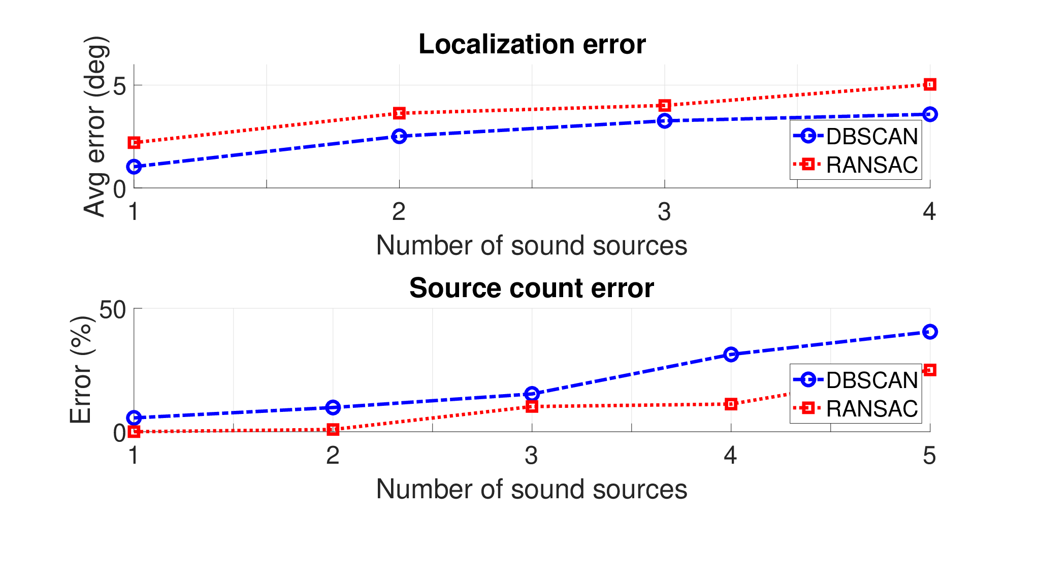
As shown in top subfigure of Fig. 15, the average error of orientation localization with the DBSCAN-based algorithm is less as compared to the RANSAC-based algorithm, which, however, generates comparatively more accurate results for source counting, as shown in the bottom subfigure of Fig. 15. In both simulations and experiments, the error of elevation angle estimation was found to be large for sources kept close to zero elevation, which coincides the conclusion in [12]. The performance of the localization and source counting using both proposed techniques can be improved by increasing the number of rotations of the bi-microphone array.
6 Conclusion and Future Scope
Two novel techniques are presented for small autonomous unmanned vehicles (SAUVs) to perform 3D multi-sound-source localization (MSSL) using a self-rotating bi-microphone array. The Density-Based Spatial Clustering of Applications with Noise (DBSCAN) based MSSL approach iteratively maps the randomly chosen points in the inter-channel time difference (ICTD) signal to the orientation domain, leading to a data sets for clustering. The number of clusters represents the number of sound sources and the location of the centroid of a cluster represents the location of a sound source. The Random Sample Consensus (RANSAC) based approach iteratively estimates parameters of a model using two randomly chosen data points from the ICTD signal data. It then uses a threshold to decide the number of qualified sound sources. The simulation and experimental results show the effectiveness of both approaches in identifying the number and the 3D orientations of the sound sources.
The techniques presented in the paper are able to localize multiple stationary sound sources by a stationary robotic platform. Considerations on the presence of obstacles and the robot/sound motions motivate our future work.
References
- (1) Q. Wang, K. Ren, M. Zhou, T. Lei, D. Koutsonikolas, and L. Su, “Messages behind the sound: real-time hidden acoustic signal capture with smartphones,” in Proceedings of the 22nd Annual International Conference on Mobile Computing and Networking. ACM, 2016, pp. 29–41.
- (2) H.-J. Böhme, T. Wilhelm, J. Key, C. Schauer, C. Schröter, H.-M. Groß, and T. Hempel, “An approach to multi-modal human–machine interaction for intelligent service robots,” Robotics and Autonomous Systems, vol. 44, no. 1, pp. 83–96, 2003.
- (3) J. C. Murray, H. Erwin, and S. Wermter, “Robotics sound-source localization and tracking using interaural time difference and cross-correlation,” in AI Workshop on NeuroBotics, 2004.
- (4) J. Borenstein, H. Everett, and L. Feng, Navigating mobile robots: systems and techniques. A K Peters Ltd., 1996.
- (5) D. V. Rabinkin, “Optimum sensor placement for microphone arrays,” Ph.D. dissertation, RUTGERS The State University of New Jersey - New Brunswick, 1998.
- (6) M. Brandstein and D. Ward, Microphone arrays: signal processing techniques and applications. Springer Science & Business Media, 2013.
- (7) H. Wallach, “On sound localization,” The Journal of the Acoustical Society of America, vol. 10, no. 4, pp. 270–274, 1939.
- (8) S. Lee, Y. Park, and Y.-s. Park, “Three-dimensional sound source localization using inter-channel time difference trajectory,” International Journal of Advanced Robotic Systems, vol. 12, no. 12, p. 171, 2015.
- (9) A. A. Handzel and P. Krishnaprasad, “Biomimetic sound-source localization,” IEEE Sensors Journal, vol. 2, no. 6, pp. 607–616, 2002.
- (10) G. H. Eriksen, “Visualization tools and graphical methods for source localization and signal separation,” Master’s thesis, Universityof OSLO, Department of Informatics, 2006.
- (11) X. Zhong, W. Yost, and L. Sun, “Dynamic binaural sound source localization with ITD cues: Human listeners,” The Journal of the Acoustical Society of America, vol. 137, no. 4, pp. 2376–2376, 2015.
- (12) D. Gala, N. Lindsay, and L. Sun, “Three-dimensional sound source localization for unmanned ground vehicles with a self-rotational two-microphone array,” in Proceedings of the 5th international conference of control, dynamic systems, and robotics (CDSR’18), 2018, pp. 104.1 – 104.11.
- (13) J.-M. Valin, F. Michaud, J. Rouat, and D. Létourneau, “Robust sound source localization using a microphone array on a mobile robot,” in Intelligent Robots and Systems, 2003.(IROS 2003). Proceedings. 2003 IEEE/RSJ International Conference on, vol. 2. IEEE, 2003, pp. 1228–1233.
- (14) L. Sun and Q. Cheng, “Indoor multiple sound source localization using a novel data selection scheme,” in 48th Annual Conference on Information Sciences and Systems (CISS). IEEE, 2014, pp. 1–6.
- (15) X. Zhong, L. Sun, and W. Yost, “Active binaural localization of multiple sound sources,” Robotics and Autonomous Systems, vol. 85, pp. 83–92, 2016.
- (16) C. Blandin, A. Ozerov, and E. Vincent, “Multi-source TDOA estimation in reverberant audio using angular spectra and clustering,” Signal Processing, vol. 92, no. 8, pp. 1950–1960, 2012.
- (17) M. Swartling, B. Sällberg, and N. Grbić, “Source localization for multiple speech sources using low complexity non-parametric source separation and clustering,” Signal Processing, vol. 91, no. 8, pp. 1781–1788, 2011.
- (18) T. Dong, Y. Lei, and J. Yang, “An algorithm for underdetermined mixing matrix estimation,” Neurocomputing, vol. 104, pp. 26–34, 2013.
- (19) O. Yilmaz and S. Rickard, “Blind separation of speech mixtures via time-frequency masking,” IEEE Transactions on signal processing, vol. 52, no. 7, pp. 1830–1847, 2004.
- (20) D. Pavlidi, A. Griffin, M. Puigt, and A. Mouchtaris, “Real-time multiple sound source localization and counting using a circular microphone array,” IEEE Transactions on Audio, Speech, and Language Processing, vol. 21, no. 10, pp. 2193–2206, 2013.
- (21) B. Loesch and B. Yang, “Source number estimation and clustering for underdetermined blind source separation,” in International Workshop on Acoustic Signal Enhancement (IWAENC), Seattle, Washington, USA, 2008.
- (22) M. C. Catalbas and S. Dobrisek, “3D moving sound source localization via conventional microphones,” Elektronika ir Elektrotechnika, vol. 23, no. 4, pp. 63–69, 2017.
- (23) J. Traa and P. Smaragdis, “Blind multi-channel source separation by circular-linear statistical modeling of phase differences,” in IEEE International Conference on Acoustics, Speech and Signal Processing (ICASSP). IEEE, 2013, pp. 4320–4324.
- (24) D. Gala and L. Sun, “Moving sound source localization and tracking using a self rotating bi-microphone array,” in ASME 2019 Dynamic Systems and Control Conference. American Society of Mechanical Engineers Digital Collection, 2019.
- (25) D. Gala, N. Lindsay, and L. Sun, “Realtime active sound source localization for unmanned ground robots using a self-rotational bi-microphone array,” Journal of Intelligent & Robotic Systems, vol. 95, no. 3-4, pp. 935–954, 2019.
- (26) M. Ester, H.-P. Kriegel, J. Sander, and X. Xu, “A density-based algorithm for discovering clusters in large spatial databases with noise,” in Kdd, vol. 96, no. 34, 1996, pp. 226–231.
- (27) C. Knapp and G. Carter, “The generalized correlation method for estimation of time delay,” IEEE Transactions on Acoustics, Speech, and Signal Processing, vol. 24, no. 4, pp. 320–327, Aug 1976.
- (28) M. Azaria and D. Hertz, “Time delay estimation by generalized cross correlation methods,” IEEE Transactions on Acoustics, Speech, and Signal Processing, vol. 32, no. 2, pp. 280–285, 1984.
- (29) P. Naylor and N. D. Gaubitch, Speech dereverberation. Springer Science & Business Media, 2010.
- (30) D. R. Gala, A. Vasoya, and V. M. Misra, “Speech enhancement combining spectral subtraction and beamforming techniques for microphone array,” in Proceedings of the International Conference and Workshop on Emerging Trends in Technology (ICWET), 2010, pp. 163–166.
- (31) D. R. Gala and V. M. Misra, “SNR improvement with speech enhancement techniques,” in Proceedings of the International Conference and Workshop on Emerging Trends in Technology (ICWET). ACM, 2011, pp. 163–166.
- (32) “International Organization for Standardization (ISO), British, European and International Standards (BSEN), Noise emitted by machinery and equipment – Rules for the drafting and presentation of a noise test code,” 12001: 1997 Acoustics.
- (33) B. Goelzer, C. H. Hansen, and G. Sehrndt, Occupational exposure to noise: evaluation, prevention and control. World Health Organisation, 2001.
- (34) L. Calmes, “Biologically inspired binaural sound source localization and tracking for mobile robots.” Ph.D. dissertation, RWTH Aachen University, 2009.
- (35) C. D. Raj, “Comparison of K means K medoids DBSCAN algorithms using DNA microarray dataset,” International Journal of Computational and Applied Mathematics (IJCAM), 2017.
- (36) N. Farmani, L. Sun, and D. J. Pack, “A scalable multitarget tracking system for cooperative unmanned aerial vehicles,” IEEE Transactions on Aerospace and Electronic Systems, vol. 53, no. 4, pp. 1947–1961, Aug 2017.
- (37) M. E. Celebi, H. A. Kingravi, and P. A. Vela, “A comparative study of efficient initialization methods for the k-means clustering algorithm,” Expert systems with applications, vol. 40, no. 1, pp. 200–210, 2013.
- (38) M. A. Fischler and R. C. Bolles, “Random sample consensus: a paradigm for model fitting with applications to image analysis and automated cartography,” Communications of the ACM, vol. 24, no. 6, pp. 381–395, 1981.
- (39) K. D. Donohue, “Audio array toolbox,” [Online] Available: http://vis.uky.edu/distributed-audio-lab/about/ , 2019, May 20.
- (40) J. B. Allen and D. A. Berkley, “Image method for efficiently simulating small-room acoustics,” The Journal of the Acoustical Society of America, vol. 65, no. 4, pp. 943–950, 1979.
- (41) K. D. Donohue, “Audio systems lab experimental data - single-track single-speaker speech,” [Online] Available: http://web.engr.uky.edu/~donohue/audio/Data/audioexpdata.htm , 2019, May 20.