The abelian antisymmetric rank 2 tensor field has a familiar gauge symmetry

$\displaystyle\delta B_{\mu\nu}=\partial_{\mu}\epsilon_{\nu}-\partial_{\nu}\epsilon_{\mu}\ .$

(2.1)

There is the residual gauge symmetry, $\delta\epsilon_{\mu}=\partial_{\mu}\eta$, which allows one to remove one component from $\epsilon_{\mu}$ and is thus important for the correct degrees of freedom count. A non-abelian generalization of (2.1) should also admit some non-abelian analog of this residual gauge symmetry. The abelian gauge-invariant 3-form field strength is $H_{\mu\nu\lambda}=\partial_{\mu}B_{\nu\lambda}+\partial_{\nu}B_{\lambda\mu}+\partial_{\lambda}B_{\mu\nu}$. To write down a gauge-invariant action in a non-abelian case, there should exist a generalized field strength that transforms covariantly.

It turns out that it is possible to construct such a model if one relaxes the condition of 6d Lorentz covariance (and locality). Our starting point will be a model involving a 6d 2-form field $B_{\mu\nu}$ in some representation of gauge group $G$ and a gauge vector field $A_{\mu}$. For the simplicity, we assume that both $B_{\mu\nu}$ and $A_{\mu}$ are taken in the adjoint representation of $G$ and use the following notation: $D_{\mu}...=\partial_{\mu}...+[A_{\mu},...],~F_{\mu\nu}=\partial_{\mu}A_{\nu}-\partial_{\nu}A_{\mu}+[A_{\mu},A_{\nu}]$. One can define the non-abelian gauge transformations as [6]

	$\displaystyle\delta A_{\mu}$	$\displaystyle=$	$\displaystyle D_{\mu}\lambda\ ,$		(2.2)
	$\displaystyle\delta B_{\mu\nu}$	$\displaystyle=$	$\displaystyle D_{\mu}\epsilon_{\nu}-D_{\nu}\epsilon_{\mu}-[F_{\mu\nu},(n^{\rho}\partial_{\rho})^{-1}(n^{\sigma}\epsilon_{\sigma})]+[B_{\mu\nu},\lambda]\ .$		(2.3)

Here $\lambda$ is the parameter of $A_{\mu}$ gauge transformations under which $B_{\mu\nu}$ transforms covariantly; $\epsilon_{\mu}$ is the parameter of the gauge transformations of $B_{\mu\nu}$, which, like $\lambda$, is now taking values in the algebra of $G$. The vector $n_{\mu}$ is a fixed constant unit vector which selects a particular direction in 6d space breaking $O(6)$ symmetry to $O(5)$. In the abelian limit, the gauge transformation (2.3) reduces to (2.1).

The structure of the non-local term in (2.3) is chosen to be such that if we further assume that $n^{\mu}A_{\mu}=0$ then there is a non-abelian generalization of the residual gauge symmetry of the parameter $\epsilon_{\mu}$ in (2.1) under which $\delta B_{\mu\nu}$ is invariant:

$\displaystyle\delta\epsilon_{\mu}=D_{\mu}\eta\ ,\qquad\qquad\delta\lambda=0\ .$

(2.4)

If we impose the additional condition that $n^{\mu}\partial_{\mu}A_{\nu}=0$, i.e. that $A_{\mu}$ depends only on 5 of the 6 coordinates (so that, in particular, $[(n^{\mu}\partial_{\mu})^{-1},D_{\nu}]f=0$ for a 6d function $f(x_{\lambda})$) then one can check that the gauge algebra closes:

$\displaystyle[\delta_{1},\delta_{2}]=\delta_{3}\ ,~~~\rm{with}~~~\quad\lambda_{3}=[\lambda_{1},\lambda_{2}]\ ,~~\quad\epsilon_{\mu 3}=[\lambda_{1},\epsilon_{\mu 2}]-[\lambda_{2},\epsilon_{\mu 1}]\ .$

(2.5)

The corresponding field strength of $B_{\mu\nu}$ is defined as

	$\displaystyle H_{\mu\nu\lambda}=D_{\mu}B_{\nu\lambda}+D_{\nu}B_{\lambda\mu}+D_{\lambda}B_{\mu\nu}$
	$\displaystyle\ \ \ \ \ \ \quad\ \ +[F_{\mu\nu},(n^{\rho}\partial_{\rho})^{-1}(n^{\sigma}B_{\lambda\sigma})]+[F_{\nu\lambda},(n^{\rho}\partial_{\rho})^{-1}(n^{\sigma}B_{\mu\sigma})]+[F_{\lambda\mu},(n^{\rho}\partial_{\rho})^{-1}(n^{\sigma}B_{\nu\sigma})]\ ,\ \ \ \ \ \$		(2.6)

where the non-local terms ensure that $H$ transforms covariantly:

$\displaystyle\delta H_{\mu\nu\sigma}=[H_{\mu\nu\sigma},\lambda]\ .$

(2.7)

Thus one can consistently couple the non-abelian antisymmetric tensor to a non-abelian gauge field restricted to a codimension-1 (“boundary”) subspace, i.e. with an effective non-locality along the “bulk” direction (see Fig.1). This non-locality may be viewed as a gauge artifact as there is a gauge in which the corresponding action is local (see below). Note also that we do not impose any boundary condition at $x_{6}=0$.

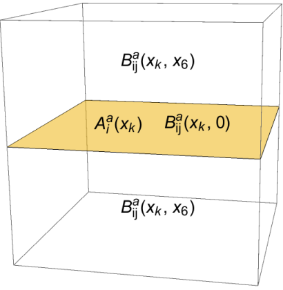
Without loss of generality, one can always choose $n_{\mu}$ to point in the 6th direction, i.e. $n_{\mu}=(0,0,0,0,0,1)$, so that the vector field restricted as above ‘‘lives’’ in 5d subspace⁴⁴ 4 We assume the Euclidean signature with 6d indices $\mu,\nu,\lambda,...=1,...,6$ and use $i,j,k,..=1,...,5$ for 5d indices.

$\displaystyle A_{\mu}=\{A_{i}(x^{k},0),\ A_{6}=0\}\ ,\quad F_{i6}=0\ ,\quad\ \ F_{ij}=\partial_{i}A_{j}-\partial_{j}A_{i}+[A_{i},A_{j}]\ ,\quad D_{6}=\partial_{6}\ .$

(2.8)

This $(B,A)$ model may be viewed as an intermediate step towards constructing an interacting model of $B$-fields only. For example, one may interpret $A$ not as an independent field but as related to $B$ by some non-local condition. In [6] the $x^{6}$ direction was assumed to be compactified to a circle of radius $R$ and $A_{i}$ was related to the zero mode of $B_{i6}$: $A_{i}\equiv\int dx^{6}\,B_{i6}=2\pi RB^{\rm{(zero~mode)}}_{i6}(x^{k})$. Moreover, the zero mode of the 3-form field strength was defined directly via the Hodge duality: $H_{ijk}(x^{k},0)\equiv{i\over 4\pi R}\epsilon_{ijkmn}F_{mn}$.⁵⁵ 5 Note that this implies $\int d^{6}x\,H^{2}_{ijk}(x^{k},0)\to{1\over R}\int d^{5}x\,F^{2}_{ij}$, which is formally consistent with scaling symmetry. The compactification assumption naturally breaks the global $SO(6)$ symmetry to $SO(5)\times SO(2)$. In the non-compact $x^{6}$ case one may set $A_{i}\equiv\int dx^{6}\,B_{i6},\ \ \lambda\equiv\int dx^{6}\,\epsilon_{6}$ and impose the boundary conditions: $\eta(x_{i},\pm\infty)=0$, $\epsilon_{i}(x_{k},\pm\infty)=[A_{i},\lambda]$, to preserve the gauge-covariant structure. One may also treat $A_{i}$ first as an independent quantum field and then integrate it out in the path integral obtaining an effective non-local model of self-coupled non-abelian $B$-fields.

Below we shall view $A_{i}$ just as a background field coupled to the quantum $B$-fields. This interacting theory will have only $SO(5)$ part of the full 6d rotational (Lorentz) symmetry.

Our starting point will be the following gauge invariant action describing the non-abelian 6d field $B_{\mu\nu}(x^{\mu})$ coupled to the 5d gauge field $A_{i}(x^{j})$:

$\displaystyle S={\textstyle{1\over 6}}\int d^{6}x~{\rm Tr\,}(H_{\mu\nu\lambda}H^{\mu\nu\lambda})\ .$

(2.9)

Here ${\rm Tr\,}$ is in some representation $R$ of gauge group, with ${\rm Tr\,}(H^{a}t^{a})^{2}=T_{R}H^{a}H^{a}$ ($a=1,...,\dim G$), with $t^{a}$ being hermitian generators and $T_{R}={\textstyle{1\over 2}}$ or $T_{R}=C_{2}$ if $H$ is a matrix with indices in fundamental or adjoint representation.

The overall (dimensionless) normalization constant in the action (2.9) will not be important as in this paper we will only consider the 1-loop approximation treating $A_{i}$ as a background field. In general, to make the model renormalizable one would need to introduce also $A$-dependent counterterms $\int d^{6}x\,[c_{1}(DF)^{2}+c_{2}F^{3}]$ (see below), i.e. two extra dimensionless coupling constants.⁶⁶ 6 In general, one could also consider adding the 5d Chern-Simons action for $A$: $S_{\rm{5d}}={\kappa\over 3}\int{\rm Tr\,}(A\wedge F\wedge F+{i\over 2}A\wedge A\wedge A\wedge F-{1\over 10}A\wedge A\wedge A\wedge A\wedge A),$ but it will not be naturally induced in the model based on (2.9) and also in its self-dual version discussed below.

From (2.6) and (2.8) we have

$\displaystyle H_{ij6}=\partial_{6}B_{ij}+D_{i}B_{j6}-D_{j}B_{i6}\ ,\qquad~~H_{ijk}=D_{i}B_{jk}+[F_{ij},\partial_{6}^{-1}B_{k6}]+{(i,j,k\rm\ cycle)}\ .$

(2.10)

The action (2.9) is invariant under gauge transformations (2.2) and (2.3), i.e.

$\displaystyle\delta B_{ij}=D_{i}\bar{\epsilon}_{j}-D_{j}\bar{\epsilon}_{i}+[B_{ij},\lambda]\ ,~~~~\delta B_{i6}=-\partial_{6}\bar{\epsilon}_{i}+[B_{i6},\lambda]\ ,~~~~\ \ \ \ \delta A_{i}=D_{i}\lambda\ ,$

(2.11)

where $\lambda=\lambda(x_{i})$ and we redefined the gauge parameter $\epsilon_{i}\to\bar{\epsilon}_{i}$ as

$\displaystyle\bar{\epsilon}_{i}=\epsilon_{i}-D_{i}\partial_{6}^{-1}\epsilon_{6}\ .$

(2.12)

We can fix the $\bar{\epsilon}_{i}$ gauge freedom by the natural gauge $B_{i6}=0$ in which the field strength becomes manifestly local

$\displaystyle B_{i6}=0:~~~~\ \ H_{ijk}=D_{i}B_{jk}+D_{j}B_{ki}+D_{k}B_{ij}\ ,~~~~\ \ \ H_{ij6}=\partial_{6}B_{ij}\ .$

(2.13)

The gauge-fixed action (2.9) is then given by

	$\displaystyle S={\textstyle{1\over 2}}\int d^{6}x~{\rm Tr\,}\big[(\partial_{6}B_{ij})^{2}+{\textstyle{1\over 3}}H^{ijk}H_{ijk}\big]={\textstyle{1\over 2}}\int d^{6}x~{\rm Tr\,}\big(B^{ij}\Delta_{ij}^{mn}B_{mn}\big)\ ,$		(2.14)
	$\displaystyle\Delta_{ij}^{mn}=-\delta^{mn}_{ij}(\partial_{6}^{2}+D^{2})+2\delta^{[m}_{[{i}}D^{n]}D_{j]}\ ,\qquad\quad D^{2}\equiv D^{i}D_{i}\ ,\quad\delta^{mn}_{ij}=\delta_{[i}^{m}\delta_{j]}^{n}\ ,$		(2.15)

where $[ij]$ stands for antisymmetrisation with weight ${\textstyle{1\over 2}}$ and $D_{i}B_{jk}\equiv\partial_{i}B_{jk}+[A_{i},B_{jk}]$.⁷⁷ 7 Note that the 6d action (2.9) or (2.14) is manifestly scale invariant. Starting with such an $(dB+AB)^{2}$ action and integrating out $A_{i}$ should give a local, scale-invariant but non-polynomial and non-Lorentz-invariant action $\sim(BB)^{-1}dBdB$ for the non-abelian $B$-fields. It will not have free quadratic part and will thus require some non-trivial (scale-invariance breaking) $B$-field background to define a perturbation theory (cf. [13]).

Our aim will be to compute the logarithmic divergences in the $A_{i}$-dependent 1-loop effective action found by integrating out the $B$-field in (2.14)⁸⁸ 8 We ignore the $A_{i}$-independent factors in the partition function $Z=e^{-\Gamma}$ that should agree with (A.4) in the free limit. See Appendix A for a discussion of the free $B$-field partition function in the “axial” gauge $B_{i6}=0$.

$\displaystyle\Gamma={\textstyle{1\over 2}}\log\det\Delta_{ij}^{mn}(A)\ .$

(2.16)

The operator $\Delta_{ij}^{mn}$ in (2.15) defined on 6d field $B_{ij}(x^{\mu})$ is, in general, non-degenerate and the gauge condition $B_{i6}=0$ does not lead to a non-trivial ($A$-dependent) ghost determinant (cf. (2.11)). Note that the gauge-fixed action (2.14) is still invariant under the following 5d local gauge transformations ($U(x^{i})\in G$):

$\displaystyle B^{\prime}_{ij}=UB_{ij}U^{-1}\ ,~~\qquad A^{\prime}_{i}=UA_{i}U^{-1}+U\partial_{i}U^{-1}\ .$

(2.17)

Provided the regularization preserves this symmetry, the effective action (2.16) should thus be built out of gauge-invariant combinations of $F_{ij}$ and $D_{i}$.

Let us now consider the analog of the non-abelian action (2.14) in the case of the $B$-field with a self-dual field strength. Let us first review the free-field case of a single self-dual field. In Minkowski signature the real 6d self-duality condition reads

$\displaystyle H_{\mu\nu\lambda}={{\textstyle{1\over 6}}}\epsilon_{\mu\nu\lambda\sigma\rho\delta}H^{\sigma\rho\delta}\ .$

(2.18)

As is well known, one way to find the action corresponding to (2.18) is to relax the manifest Lorentz symmetry. A systematic approach is to start with the phase-space path integral for the non-chiral $H^{2}_{\mu\nu\lambda}$ theory, impose the standard “time-like” gauge $B_{i0}=0$, trade the momenta corresponding to $B_{ij}$ for another 2-form field and then impose the self-duality truncation ending up with the “${\cal EB-BB}$” type action ($\cal E$ is “electric” and $\cal B$ is “magnetic”) [14] (see also [15, 16, 17, 18]).⁹⁹ 9 To get the right count of degrees of freedom at the level of path integral one should also keep track of appropriate Jacobians in the path integral measure. Switching to the Euclidean notation that we shall use below ($x^{0}\to ix^{6}$, with the gauge condition $B_{i6}=0$) the resulting action is ($i,j,...=1,...,5$)

$\displaystyle\tilde{S}_{+}=\int d^{6}x~\,{\textstyle{1\over 2}}i\,\epsilon_{ijkpq}\partial_{k}B_{pq}\big(\partial_{6}B_{ij}+{\textstyle{1\over 2}}i\,\epsilon_{ijrmn}\partial_{r}B_{mn}\big)\ .$

(2.19)

It formally has a residual gauge invariance $\delta B_{ij}=\partial_{i}\xi_{j}-\partial_{j}\xi_{i}$.¹⁰¹⁰ 10 This a 6d symmetry; the action is invariant up to a surface term. This residual symmetry is an artifact of the action (2.19) – it is absent in the required self-duality equation ${\cal O}_{+}B_{ij}=0$. Taking the variation of (2.19) over $B_{ij}$ we obtain the equation of motion which may be written as¹¹¹¹ 11 As in (2.15), we adopt the standard convention $\delta^{mn}_{ij}={1\over 2}(\delta_{i}^{m}\delta_{j}^{n}-\delta_{i}^{n}\delta_{j}^{m})$.

$\displaystyle\partial_{[k}{\cal O}_{+}B_{ij]}=0\ ,\qquad\qquad({\cal O}_{\pm})_{ij,mn}\equiv\delta_{ij,mn}\partial_{6}\pm{\textstyle{1\over 2}}i\,\epsilon_{ijrmn}\partial_{r}\ .$

(2.20)

It is solved by

$\displaystyle{\cal O}_{+}B_{ij}=\partial_{i}q_{j}(x_{i})-\partial_{j}q_{i}(x_{i})+f_{ij}(x^{6})\ ,$

(2.21)

for a 5d function $q_{i}(x_{i})$ and a function $f_{ij}(x^{6})$ that does not depend on 5d coordinates. Absorbing $q_{i}$ part into a formal redefinition of $B_{ij}$ in $\partial_{6}B_{ij}$ term in ${\cal O}_{+}B_{ij}$ and imposing the boundary condition that the self-duality condition ${\cal O}_{+}B_{ij}=0$ is satisfied at “spatial infinity” $|x^{i}|=\infty$ we conclude that $f_{ij}=0$ and thus ${\cal O}_{+}B_{ij}=0$ is satisfied everywhere. Integrating over $B_{ij}$ in the path integral defined by the action (2.19) and taking into account the necessary determinant factors in the measure one finds that the resulting partition function is

$\displaystyle Z_{+}=\big(\det{\cal O}^{\perp}_{+}\big)^{-1/2}\ ,$

(2.22)

where ${\cal O}_{+}^{\perp}$ acts on transverse $B^{\perp}_{ij}$ field and thus describes 3 dynamical degrees of freedom as expected.¹²¹² 12 $B^{\perp}_{ij}$ has ${\textstyle{1\over 2}}\times 4\times 5-(5-1)=6$ real components and that the differential operator is a 1-st order one (cf. Appendix A).

The equivalent results can be obtained by starting with an alternative (“$\cal EB-EE$”) action

$\displaystyle S_{+}=\int d^{6}x\,\partial_{6}B_{ij}\big(\partial_{6}B_{ij}+{\textstyle{1\over 2}}i\,\epsilon_{ijkmn}\partial_{k}B_{mn}\big)\ .$

(2.23)

Here the equations of motion $\partial_{6}({\cal O}_{+}B_{ij})=0$ reduce to ${\cal O}_{+}B_{ij}=f_{ij}(x^{k}),$ and thus if the self-duality condition ${\cal O}_{+}B_{ij}=0$ is imposed at $|x^{6}|=\infty$, it is satisfied everywhere. The action (2.23) has a 5d residual gauge symmetry $\delta B_{ij}=\partial_{i}\xi_{j}-\partial_{j}\xi_{i}$, where $\xi_{i}=\xi_{i}(x^{k})$. The $B_{ij}$ path integral measure here should have an extra factor of $(\det\partial_{6})^{1/2}$ that ensures 6d Lorentz invariance; as a result one finds the same chiral partition function (2.22) (cf. Appendix A).

Note that the free limit of the non-chiral action (2.14) is equivalent to a combination of the self-dual and anti self-dual models: in the free limit the kinetic term in (2.14),(2.15) may be written as

$\displaystyle(\partial_{6}B_{ij})^{2}+{\textstyle{1\over 3}}H^{ijk}H_{ijk}={\cal O}_{+}B_{ij}\,{\cal O}_{-}B_{ij}\ ,\ \ \ \$

(2.24)

and thus the corresponding partition function is given by

$\displaystyle Z=(\det\Delta_{\perp})^{-1/2}=Z_{+}Z_{-}\ .$

(2.25)

The above discussion has a straightforward generalization to the non-abelian case. Namely, let us require that the self-duality condition (2.18) or its Euclidean counterpart in the $B_{i6}=0$ gauge should be satisfied for the non-abelian field strength (2.6) or (2.10), i.e.

$\displaystyle\hat{\cal O}_{+}B_{ij}=0\ ,\qquad\qquad(\hat{\cal O}_{\pm})_{ij,mn}\equiv\delta_{ij,mn}\partial_{6}\pm{\textstyle{1\over 2}}i\,\epsilon_{ijkmn}D_{k}(A)\ .$

(2.26)

One may expect that this condition should follow (under the corresponding boundary conditions discussed above) from the direct analogs of (2.23) and (2.19):

	$\displaystyle S_{+}=\int d^{6}x\,{\rm Tr\,}\Big[\,\partial_{6}B_{ij}\big(\partial_{6}B_{ij}+{\textstyle{1\over 2}}i\,\epsilon_{ijkmn}D_{k}B_{mn}\big)\Big]\ ,\$		(2.27)
	$\displaystyle\tilde{S}_{+}=\int d^{6}x\,{\rm Tr\,}\Big[\,{\textstyle{1\over 2}}i\,\epsilon_{ijrpq}D_{r}B_{pq}\big(\partial_{6}B_{ij}+{\textstyle{1\over 2}}i\,\epsilon_{ijkmn}D_{k}B_{mn}\big)\Big]\ .\$		(2.28)

This is indeed obvious for (2.27) but is not immediately so for the second action (2.28). The equations of motion following from (2.28), $D_{[i}\hat{\cal O}_{+}B_{jk]}=0$, may be solved as $\hat{\cal O}_{+}B_{ij}=q(x^{6})F_{ij}(x^{k})+f_{ij}(x^{6})$, where $F_{ij}$ is the field strength of $A_{i}$. One may then attempt to absorb the $F$-term by a (non-local in $x^{6}$) redefinition $B_{ij}\to B_{ij}+(\partial_{6})^{-1}q(x^{6})F_{ij}(x^{k})$ to arrive at the self-duality condition. However, the quantum equivalence of the theories based on (2.27) and (2.28) becomes unclear as an extra determinant of the operator ${\textstyle{1\over 2}}i\,\epsilon_{ijrpq}D_{r}$ coming from (2.28) will now have a non-trivial dependence on $A_{i}$.

In what follows we shall use the simplest action (2.27) as defining the non-abelian self-dual $B$-field model.¹³¹³ 13 Like the free action (2.23) the interacting action (2.27) still has the residual 5d gauge symmetry $\delta B_{ij}=\partial_{i}\xi_{j}-\partial_{j}\xi_{i}$, $\xi_{i}=\xi_{i}(x^{k},0)$ under which the variation of (2.27) is a total derivative: $\delta S_{+}={\rm Tr\,}\int d^{6}x\,\,\partial_{6}B_{ij}\big(i\,\epsilon_{ijkmn}[A_{k},\partial_{m}\xi_{n}]\big)={\rm Tr\,}\int d^{6}x\,\,\partial_{6}\big(B_{ij}i\,\epsilon_{ijkmn}[A_{k},\partial_{m}\xi_{n}]\big)$. Since the parameter does not depend on $x^{6}$, this does not imply a degeneracy of the resulting kinetic operator for generic values of 6-momentum and thus does not require gauge fixing. Since the $\partial_{6}$ operator factorizes in (2.27), the corresponding partition function is given by the direct analog of (2.22) with ${\cal O}_{+}\to\hat{\cal O}_{+}(A)$.¹⁴¹⁴ 14 As in (2.16) we shall ignore constant $A$-independent factors in $Z$: the operator $\hat{\cal O}_{+}$ is acting on the full $B_{ij}$ rather than on its transverse part as in the free case in (2.22). It is straightforward to check that the operator $\Delta(A)$ in the non-chiral action (2.14),(2.15) is given again by the product of the self-dual and anti self-dual operators in (2.26):

$\displaystyle\Delta^{mn}_{ij}(A)=-\hat{\cal O}^{\ mn}_{+\,pq}(A)\ \hat{\cal O}^{\ pq}_{-\,ij}(A)\ .$

(2.29)

As a result, the non-chiral $B$-field quantum effective action (2.16) may be written as

$\displaystyle\Gamma=\Gamma_{+}+\Gamma_{-}\ ,\ \ \qquad\qquad\Gamma_{\pm}={\textstyle{1\over 2}}\log\det\hat{\cal O}_{\pm}(A)\ .$

(2.30)

While $\Gamma$ should be parity (P) even, $\Gamma_{+}$ and $\Gamma_{-}$ may a priori contain imaginary P-odd parts that cancel in their sum in (2.26) (as, e.g., in the case of an external gravitational field [11]). However, it is easy to see that this does not happen in the present case when the external field $A_{i}$ does not depend on $x^{6}$. Indeed, $\partial_{6}\to-\partial_{6}$ combined with $\epsilon_{5}\to-\epsilon_{5}$ is a symmetry of the classical action (2.27) and thus should be present also in the effective action. As the P-odd part of $\Gamma_{\pm}$ should contain an odd number of $\epsilon_{5}=(\epsilon_{ijkmn})$ factors it should thus have an odd number of $p_{6}$ factors (in momentum representation) but then the integral over $p_{6}$ vanishes. The absence of P-odd part implies also the absence of an anomalous (5d gauge symmetry breaking) part of $\Gamma_{\pm}$. Thus both the effective action $\Gamma$ of the full non-chiral theory and $\Gamma_{+}$ of the self-dual theory should be invariant under the residual gauge symmetry of the $A$-field in (2.17).

To conclude, we have

$\displaystyle\Gamma=2\Gamma_{+}\ ,\ \ \qquad\qquad\Gamma_{+}=\Gamma_{-}={\textstyle{1\over 2}}\log\det\hat{\cal O}_{+}(A)\ .$

(2.31)

The effective action corresponding to the classical action (2.27) is¹⁸¹⁸ 18 Compared to (2.30),(2.31) here we include the $A$-independent factor $\partial_{6}$ in the kinetic operator making it symmetric.

$\displaystyle\Gamma_{+}={\textstyle{1\over 2}}\log\det\Delta_{+}\ ,\qquad\qquad\Delta_{+}B_{ij}=-\partial_{6}\hat{\cal O}_{+}B_{ij}=-\partial_{6}(\partial_{6}B_{ij}+\textstyle{i\over 2}\epsilon_{ijkmn}D_{k}B_{mn})\ .$

(4.1)

The operator $\Delta_{+}$ is thus linear in the background field $A_{i}$, i.e.¹⁹¹⁹ 19 Here $a,b,c$ are Lie algebra indices. We assume that $B$ is in adjoint representation; otherwise $t^{a}_{bc}=-if^{a}_{\ bc}$ is to be replaced by the corresponding hermitian generators.

		$\displaystyle\Delta_{+}=\Delta^{(0)}+\Delta^{(1)}\ ,\qquad$		(4.2)
		$\displaystyle[\Delta^{(0)}]^{ab}_{ij,mn}=\textstyle-\delta^{ab}\big(\delta_{ij,mn}\partial^{2}_{6}+{i\over 2}\epsilon_{ijkmn}\partial_{6}\partial_{k}\big)\ ,\qquad[\Delta^{(1)}]^{ab}_{ij,mn}=-{i\over 2}f^{acb}\epsilon_{ijkmn}A^{c}_{k}\partial_{6}\ .$		(4.3)

Expanding the non-trivial part of $\Gamma_{+}$ in powers of $A$, we have

	$\displaystyle\textstyle\Gamma_{+}=\Gamma_{2}+\Gamma_{3}+....\ ,\qquad$		$\displaystyle\textstyle\Gamma_{2}=-{1\over 4}\mathop{\mathrm{tr}}\big[(\Delta^{(0)})^{-1}\Delta^{(1)}(\Delta^{(0)})^{-1}\Delta^{(1)}\big]\ ,$		(4.4)
			$\displaystyle\textstyle\Gamma_{3}={1\over 6}\mathop{\mathrm{tr}}\big[(\Delta^{(0)})^{-1}\Delta^{(1)}(\Delta^{(0)})^{-1}\Delta^{(1)}(\Delta^{(0)})^{-1}\Delta^{(1)}\big]\ .$

Since the background field $A_{i}$ is independent of $x_{6}$, the trace projects out all terms containing an odd number of $\partial_{6}$ factors and also produces an overall factor of length $L_{6}=\int dx_{6}$. As was already mentioned in section 2, together with the symmetry of the gauge-fixed action (2.27) under $\partial_{6}\rightarrow-\partial_{6}$ combined with $\epsilon_{5}\rightarrow-\epsilon_{5}$, this implies the effective action $\Gamma_{+}$ is parity-even.

The evaluation of traces is standard, by using momentum space basis of states and assuming that the background field is $A_{i}^{a}(x_{k})=\int{d^{5}s\over(2\pi)^{5}}\tilde{A}_{i}^{a}(s)e^{is_{k}x_{k}}.$ The matrix element of $(\Delta^{(0)})^{-1}$ in momentum representation is the free $B$-field propagator

	$\displaystyle\langle p|(\Delta^{(0)})^{-1}|p\rangle\ \to\ \delta^{ab}\ P^{jk}_{mn}(p_{i},p_{6})\ ,$
	$\displaystyle P^{jk}_{mn}(p_{i},p_{6})\equiv{1\over(p_{i}^{2}+p^{2}_{6})}\Big(\delta^{jk}_{mn}-{\textstyle{i\over 2}}{\epsilon_{mnq}^{~~~~~jk}p_{q}\over p_{6}}+2{p^{[j}p_{[m}\delta^{k]}_{n]}\over p^{2}_{6}}\Big)\ .$		(4.5)

The matrix element of $\Delta^{(1)}$ is the vertex

$\displaystyle\langle p+s|\Delta^{(1)}|p\rangle\ \to\ V_{ij}^{ab\ mn}(s_{i},p_{6})\equiv{\textstyle{1\over 2}}f^{acb}\epsilon_{ij}{}^{kmn}p_{6}\tilde{A}^{c}_{k}(s_{i})\ .$

(4.6)

References

- [1] C. Saemann and L. Schmidt, “Towards an M5-Brane Model I: A 6d Superconformal Field Theory,” J. Math. Phys. 59, 043502 (2018) [arXiv:1712.06623].
- [2] H. Samtleben, E. Sezgin and R. Wimmer, “(1,0) superconformal models in six dimensions,” JHEP 1112, 062 (2011) [arXiv:1108.4060]; “Six-dimensional superconformal couplings of non-abelian tensor and hypermultiplets,” JHEP 1303, 068 (2013) [arXiv:1212.5199]. H. Samtleben, E. Sezgin, R. Wimmer and L. Wulff, “New superconformal models in six dimensions: Gauge group and representation structure,” PoS Corfu 2011, 071 (2011) [arXiv:1204.0542].
- [3] N. Lambert and C. Papageorgakis, “Nonabelian (2,0) Tensor Multiplets and 3-algebras,” JHEP 1008, 083 (2010) [arXiv:1007.2982 [hep-th]].
- [4] C.-S. Chu and S.-L. Ko, “Non-abelian Action for Multiple Five-Branes with Self-Dual Tensors,” JHEP 1205, 028 (2012) [arXiv:1203.4224 [hep-th]].
- [5] F. Bonetti, T. W. Grimm and S. Hohenegger, “Non-Abelian Tensor Towers and (2,0) Superconformal Theories,” JHEP 1305, 129 (2013) [arXiv:1209.3017 [hep-th]].
- [6] P.-M. Ho, K.-W. Huang and Y. Matsuo, “A Non-Abelian Self-Dual Gauge Theory in 5+1 Dimensions,” JHEP 1107, 021 (2011) [arXiv:1104.4040].
- [7] P.-M. Ho and Y. Matsuo, “Note on non-Abelian two-form gauge fields,” JHEP 1209, 075 (2012) [arXiv:1206.5643]. “Aspects of Effective Theory for Multiple M5-Branes Compactified On Circle,” JHEP 1412, 154 (2014) [arXiv:1409.4060].
- [8] K.-W. Huang, “Non-Abelian Chiral 2-Form and M5-Branes,” arXiv:1206.3983.
- [9] E. S. Fradkin and A. A. Tseytlin, “Quantum Properties of Higher Dimensional and Dimensionally Reduced Supersymmetric Theories,” Nucl. Phys. B 227, 252 (1983).
- [10] P. H. Frampton and T. W. Kephart, “Explicit Evaluation of Anomalies in Higher Dimensions,” Phys. Rev. Lett. 50, 1343 (1983) Erratum: [Phys. Rev. Lett. 51, 232 (1983)].
- [11] L. Alvarez-Gaume and E. Witten, “Gravitational Anomalies,” Nucl. Phys. B 234 (1984) 269
- [12] F. Bastianelli and P. van Nieuwenhuizen, “Gravitational Anomalies From the Action for Selfdual Antisymmetric Tensor Fields in (4k+2)-dimensions,” Phys. Rev. Lett. 63, 728 (1989).
- [13] M. Beccaria and A. A. Tseytlin, “Partition function of free conformal fields in 3-plet representation,” JHEP 1705, 053 (2017) [arXiv:1703.04460].
- [14] M. Henneaux and C. Teitelboim, “Dynamics of Chiral (Selfdual) Forms,” Phys. Lett. B 206, 650 (1988).
- [15] J. H. Schwarz and A. Sen, “Duality symmetric actions,” Nucl. Phys. B 411, 35 (1994) [hep-th/9304154].
- [16] M. Perry and J. H. Schwarz, “Interacting chiral gauge fields in six-dimensions and Born-Infeld theory,” Nucl. Phys. B 489, 47 (1997) [hep-th/9611065].
- [17] P. Pasti, D. P. Sorokin and M. Tonin, “On Lorentz invariant actions for chiral p forms,” Phys. Rev. D 55, 6292 (1997) [hep-th/9611100].
- [18] D. Belov and G. W. Moore, “Holographic Action for the Self-Dual Field,” [hep-th/0605038].
- [19] P. B. Gilkey, “The Spectral geometry of a Riemannian manifold,” J. Diff. Geom. 10, no. 4, 601 (1975).
- [20] F. Bastianelli, S. Frolov and A. A. Tseytlin, “Conformal anomaly of (2,0) tensor multiplet in six-dimensions and AdS/CFT correspondence,” JHEP 0002, 013 (2000) [hep-th/0001041].
- [21] H. Osborn and A. Stergiou, “Structures on the Conformal Manifold in Six Dimensional Theories,” JHEP 1504, 157 (2015) [arXiv:1501.01308].
- [22] E. A. Ivanov, A. V. Smilga and B. M. Zupnik, “Renormalizable supersymmetric gauge theory in six dimensions,” Nucl. Phys. B 726, 131 (2005) [hep-th/0505082]. A. V. Smilga, “Chiral anomalies in higher-derivative supersymmetric 6D theories,” Phys. Lett. B 647, 298 (2007) [hep-th/0606139].
- [23] I. L. Buchbinder, E. A. Ivanov, B. S. Merzlikin and K. V. Stepanyantz, “One-loop divergences in 6D, = (1, 0) SYM theory,” JHEP 1701, 128 (2017) [arXiv:1612.03190]; “Supergraph analysis of the one-loop divergences in , and gauge theories,” Nucl. Phys. B 921, 127 (2017) [arXiv:1704.02530]. E. Ivanov, “Classical and quantum superfield invariants in SYM theory,” J. Phys. Conf. Ser. 965, no. 1, 012021 (2018).
- [24] J. Bhattacharya and A. E. Lipstein, “6d Dual Conformal Symmetry and Minimal Volumes in AdS,” JHEP 1612, 105 (2016) [arXiv:1611.02179 [hep-th]].
- [25] R. Manvelyan and A. C. Petkou, “The Trace anomaly of the (2,0) tensor multiplet in background gauge fields,” JHEP 0006, 003 (2000) [hep-th/0005256].
- [26] A. S. Schwarz, “The Partition Function of a Degenerate Functional,” Commun. Math. Phys. 67, 1 (1979). A. S. Schwarz and Y. S. Tyupkin, “Quantization Of Antisymmetric Tensors And Ray-singer Torsion,” Nucl. Phys. B 242, 436 (1984).
- [27] M. Beccaria, X. Bekaert and A. A. Tseytlin, “Partition function of free conformal higher spin theory,” JHEP 1408, 113 (2014) [arXiv:1406.3542].