Joint analysis of the thermal Sunyaev-Zeldovich effect and 2MASS galaxies: Probing gas physics in the local Universe and beyond
Abstract
We present a first joint analysis of the power spectra of the thermal Sunyaev-Zeldovich (tSZ) effect measured by the Planck and the number density fluctuations of galaxies in the 2MASS redshift survey (2MRS) catalog, including their cross-correlation. Combining these measurements with the cosmic microwave background (CMB) data and CMB lensing of Planck assuming a flat CDM model, we constrain the mass bias parameter as [, where ], i.e., the Planck cluster mass should be lower than the true mass. The mass bias determined by the 2MRS-tSZ cross-power spectrum alone is consistent with that determined by the tSZ auto-power spectrum alone, suggesting that this large mass bias is not due to obvious systematics in the tSZ data. We find that the 2MRS-tSZ cross-power spectrum is more sensitive to less massive halos than the tSZ auto-power spectrum and it significantly improves a constraint on the mass dependence of the mass bias. The redshift dependence is not strongly constrained since the multipole range in which high redshift clusters mainly contribute to the tSZ auto is dominated by the contaminating sources. We conclude that no strong mass or redshift evolution of the mass bias is needed to explain the data.
Keywords:
galaxies: clusters: general - galaxies: clusters: intracluster medium - cosmic background radiation - cosmological parameters - cosmology: theory1 Introduction
The angular power spectrum of the thermal Sunyaev-Zel’dovich (tSZ) effect (Sunyaev & Zeldovich 1972) is very sensitive to the amplitude of matter density fluctuation, which is characterized by the cosmological parameters and (Komatsu & Kitayama 1999; Komatsu & Seljak 2002).
Recently the Planck satellite provided an all-sky map of the tSZ effect and its angular power spectrum (Planck Collaboration et al. 2016b). With this, they put a constraint on the combination of the cosmological parameters, , independently from the primordial CMB fluctuation. However, the derived value of depends on the so-called mass bias parameter , which is introduced to account for the uncertainty in the cluster mass estimation in the Planck analysis. It is defined as the ratio of the Planck cluster mass and the true mass,
| (1) |
where is the mass enclosed by the radius within which the average mass density is 500 times of the critical density of the Universe. The mass bias is related to the more commonly used parameter as .
Using the gas pressure profile of Arnaud et al. (2010), which is estimated from a local cluster sample observed by XMM-Newton assuming the hydrostatic equilibrium (HSE), Planck Collaboration et al. (2016b) reported that – is required to reconcile the tSZ power spectrum with the combined constraints from the primordial CMB fluctuation, CMB lensing and baryon acoustic oscillations. Several authors performed a revised analysis of the tSZ power spectrum and obtained similar results (Horowitz & Seljak 2017; Hurier & Lacasa 2017; Salvati et al. 2018; Bolliet et al. 2018). From the simulation side, Dolag et al. (2016) constructed the tSZ map from their Magneticum Pathfinder Simulations and found that the mass bias of gives a reasonable agreement with the observations.
It has been thought that the mass bias mainly arises from the assumption of the HSE with thermal pressure. The hydrodynamic simulations showed that the HSE mass underestimates the true mass by 5–20% due to non-thermal pressure support (e.g., Kay et al. 2004; Rasia et al. 2006; Rasia et al. 2012; Nagai et al. 2007a; Piffaretti & Valdarnini 2008; Lau et al. 2009; Meneghetti et al. 2010; see also Shi & Komatsu 2014; Shi et al. 2015; Shi et al. 2016). Other effects such as the calibration error of gas temperature in X-ray observations may also contribute to the mass bias (Schellenberger et al. 2015).
There are several surveys that have attempted to calibrate cluster masses by weak gravitational lensing assuming that the lensing mass is unbiased (von der Linden et al. 2014; Hoekstra et al. 2015; Smith et al. 2016; Penna-Lima et al. 2017; Medezinski et al. 2018; Sereno et al. 2017). The derived mass biases differ among those surveys. Some studies found consistent results with the Planck, but the other studies favored a smaller bias (–). Since the cluster samples in those surveys have different masses and redshift ranges, it is still unclear whether the differences between surveys come from systematic uncertainties or the mass and/or redshift evolution of the mass bias (Andreon 2014; Sereno & Ettori 2017).
The cross-correlation technique offers a promising way to address this issue. Taking the cross-correlation between the tSZ map and other observables whose mass and redshift distribution is different from the tSZ effect provides us tomographic information. It also enables us to check consistency between data sets. Another advantage is that the cross-correlation measurements are free from contamination in the tSZ map if the contamination does not correlate with the respective observables. The uniqueness and effectiveness of the cross-correlation technique are proven by recent studies on the cross-correlation of the tSZ with, e.g., weak lensing shear/convergence field (Hill & Spergel 2014; Van Waerbeke et al. 2014; Ma et al. 2015; Hojjati et al. 2017; Osato et al. 2018), X-ray clusters (Hajian et al. 2013), and galaxy groups from the Sloan Digital Sky Survey (Vikram et al. 2017).
In this paper, we present a first joint analysis of the power spectra of the tSZ effect and the number density fluctuations of galaxies in the 2MASS redshift survey (2MRS; Huchra et al. 2012), which is a spectroscopic follow-up of Two Micron All Sky Survey (Skrutskie et al. 2006), including their cross-correlation. The angular auto-power spectrum of the 2MRS galaxies is dominated by galaxies living inside nearby groups and clusters (Ando et al. 2018). By cross-correlating them with the tSZ map, we can investigate physical properties of hot gas in the nearby halos and their relation with galaxy distributions. It may also provide a good constraint on the local universe simulations, e.g., the Magneticum Pathfinder simulation (Dolag et al. 2016) and ELUCID (Wang et al. 2014).
This paper is organized as follows. In Section 2 we describe the data sets and measurement of auto- and cross-power spectra. In Section 3 we outline the model of power spectra. In Section 4 we perform a joint analysis and obtain constraints on the model parameters and discuss their implications for gas physics. We summarize our results in Section 5. In Appendix A we investigate the effect of the tSZ map reconstruction methods. In Appendix B we describe systematic uncertainties in the covariance matrix estimation. Throughout the paper, we assume a flat -CDM cosmology.
2 Data sets
2.1 Construction of the maps
2.1.1 Compton-Y
The tSZ effect is characterized by the Compton-Y parameter, which is defined as (Sunyaev & Zeldovich 1972)
| (2) |
where is the Boltzmann constant, is the electron mass, is the speed of light, is the Thomson scattering cross section, is the distance along the line of sight, and and are the electron density and temperature. The temperature distortion of the cosmic microwave background (CMB) caused by the tSZ effect at a frequency is given by
| (3) |
Neglecting relativistic corrections, with and K.
For the tSZ data, we use the full sky Compton-Y map provided in the Planck 2015 public data release (Planck Collaboration et al., 2016b). The Planck public data include two Compton-Y maps, namely, MILCA and NILC, which use different map reconstruction methods. We estimate the cross-power spectra between the 2MRS map and both Compton-Y maps and find that they agree with each other within the error (see Appendix A for details). In the rest of this paper, we show the results for the NILC map unless otherwise noted.
The tSZ map is contaminated by the strong thermal dust emission from our Galaxy as well as by emission of the infrared (IR) and radio point sources. To reduce the contamination we apply the Galactic mask, which masks of the sky, and the point source mask provided by the Planck. Combining the Galactic mask and the point source mask, the fraction of the sky available for analysis becomes .
2.1.2 2MRS
We use the galaxy catalog obtained by the 2MRS (Huchra et al. 2012). Figure 1 shows the redshift distribution of the 2MRS galaxies, which is well modeled as
| (4) |
with , , and (Ando et al., 2018). The total number of the galaxies in the 2MRS catalogue in the unmasked pixels is = 43182. The median redshift of the 2MRS galaxies is .
From the catalog we construct the pixel-based density fluctuation map of the 2MRS galaxies using the HEALPix11 1 http://healpix.jpl.nasa.gov (Górski et al., 2005) package, at the same pixel resolution as the Planck Compton-Y map, . The density fluctuation of galaxies is defined as
| (5) |
where is the mean number of galaxies per pixel outside the mask, and is the number of galaxies in a given pixel.
Following Ando et al. (2018), we mask the Galactic plane region and the small regions in which the redshift completeness is low (Lavaux & Hudson 2011). With this mask, the sky fraction of the 2MRS galaxy density map is .
For further details of the map construction methods and clustering properties of the 2MRS galaxies, see Ando et al. (2018).

.
2.2 Power spectra
To compute tSZ auto-, 2MRS auto- and tSZ-2MRS cross-power spectra, we use the public code anafast in the HEALPix package (Górski et al. 2005). The mode coupling effect induced by the mask is corrected by the MASTER algorithm (Hivon et al., 2002). We use the cross power spectrum of the tSZ and 2MRS masks to correct the masking effect in the tSZ-2MRS cross power spectrum. The pixelization and beam smearing effects are corrected by dividing the measured power spectra by the square of the window function ,
| (6) |
where is the pixel window function for and is the beam window function of the Planck. We assume that the Planck beam is approximated by a circular Gaussian with the FWHM of (Planck Collaboration et al., 2016b).
In the following, we denote an angular power spectrum between observables and as . For example, the galaxy auto power spectrum is written as , while the galaxy-tSZ cross power spectrum is . We bin all the power spectra in 19 bins that are logarithmically equally spaced in multipole (covering ), weighted by .
The measured power spectra are summarized in Table 1.
2.2.1 The tSZ auto power spectrum
Following Planck Collaboration et al. (2016b), we cross-correlate Compton-Y maps from the first and second halves of the data to obtain the angular auto power spectrum of the tSZ signal.
While the cross-correlation between the first and second halves of the data reduces the instrumental noise bias, there still remains some contamination from the cosmic infrared background (CIB) and residual IR and radio point sources. In the analysis of the power spectra, we take into account the contamination from those sources (see Section 3.1.1 and 4.2 for details).
2.2.2 The 2MRS auto power spectrum
The galaxy auto power spectrum is measured from the density fluctuation map described in Section 2.1.2 by also using anafast and MASTER. We employ the same procedure as in Ando et al. (2018) to subtract the shot noise term. First, we randomly divide the galaxy catalog into two subsets, both of which contain roughly the same number of galaxies. Then we convert these two subsets into the density fluctuation map, and , and construct a half-sum (HS) and a half-difference (HD) map from them:
| (7) |
Since the power spectrum measured from the HS map contains both signal and noise while that from the HD map contains only noise, the galaxy auto power spectrum is estimated as
| (8) |
In the top panel of Figure 2 we show the measured galaxy auto power spectrum.
2.2.3 The tSZ-2MRS cross power spectrum
We use anafast and MASTER to measure the tSZ-galaxy cross power spectrum from the Planck full mission Compton-Y map and the HS map of the 2MRS galaxies.
In the bottom panel of Figure 2 we show the measured tSZ-galaxy cross power spectrum. The signal is detected with the signal-to-noise ratio of 9.92 (), which is calculated as
| (9) |
where is the covariance matrix of the cross-power spectrum described in Section 4.1.
As shown in Planck Collaboration et al. (2016b), contaminations from the CIB and IR and radio point sources begin to dominate the angular power spectrum of Compton-Y at higher multipoles. As the CIB is thought to mainly come from relatively higher redshift (), it should not correlate with the 2MRS galaxies in the local universe (). On the other hand, the redshift distribution of the residuals of IR and radio point sources are still unclear and it could correlate with the 2MRS sources. Thus we decide not to use at in the parameter fitting.


.
| 10 | 7.18e-03 | 1.42e-03 | 3.28e-04 | 2.68e-16 | 1.52e-16 | 8.83e-15 | 4.37e-10 | 2.31e-10 | 6.06e-10 |
|---|---|---|---|---|---|---|---|---|---|
| 13 | 5.18e-03 | 7.77e-04 | 2.65e-04 | 5.59e-16 | 1.47e-16 | 4.32e-15 | 3.55e-10 | 2.08e-10 | 4.03e-10 |
| 18 | 3.84e-03 | 4.52e-04 | 2.09e-04 | 4.32e-16 | 1.13e-16 | 2.08e-15 | 4.34e-10 | 1.27e-10 | 2.69e-10 |
| 23 | 2.42e-03 | 2.39e-04 | 1.61e-04 | 3.92e-16 | 8.12e-17 | 1.06e-15 | 3.72e-10 | 7.94e-11 | 1.81e-10 |
| 30 | 1.66e-03 | 1.31e-04 | 1.21e-04 | 2.25e-16 | 3.63e-17 | 5.49e-16 | 2.07e-10 | 3.87e-11 | 1.21e-10 |
| 40 | 1.27e-03 | 7.74e-05 | 8.63e-05 | 1.34e-16 | 1.76e-17 | 2.79e-16 | 1.59e-10 | 2.02e-11 | 7.82e-11 |
| 52 | 9.71e-04 | 4.85e-05 | 5.96e-05 | 1.10e-16 | 9.90e-18 | 1.41e-16 | 1.04e-10 | 1.26e-11 | 4.90e-11 |
| 68 | 7.68e-04 | 3.13e-05 | 4.05e-05 | 6.44e-17 | 5.00e-18 | 7.28e-17 | 7.04e-11 | 6.92e-12 | 3.02e-11 |
| 89 | 5.15e-04 | 1.76e-05 | 2.68e-05 | 5.05e-17 | 3.10e-18 | 3.74e-17 | 4.95e-11 | 4.05e-12 | 1.79e-11 |
| 117 | 3.86e-04 | 1.14e-05 | 1.73e-05 | 4.78e-17 | 2.17e-18 | 1.92e-17 | 3.38e-11 | 2.77e-12 | 1.02e-11 |
| 152 | 2.88e-04 | 7.39e-06 | 1.10e-05 | 3.33e-17 | 1.38e-18 | 9.89e-18 | 2.41e-11 | 1.70e-12 | 5.64e-12 |
| 198 | 2.04e-04 | 4.90e-06 | 6.86e-06 | 2.32e-17 | 8.45e-19 | 5.16e-18 | 1.59e-11 | 1.05e-12 | 3.00e-12 |
| 257 | 1.45e-04 | 3.26e-06 | 4.19e-06 | 1.85e-17 | 5.73e-19 | 2.68e-18 | 9.35e-12 | 6.91e-13 | 1.52e-12 |
| 335 | 1.02e-04 | 2.23e-06 | 2.52e-06 | 1.32e-17 | 4.03e-19 | 1.38e-18 | 6.43e-12 | 4.52e-13 | 7.23e-13 |
| 436 | 7.41e-05 | 1.60e-06 | 1.50e-06 | 9.29e-18 | 2.80e-19 | 7.17e-19 | 3.56e-12 | 3.07e-13 | 3.28e-13 |
| 567 | 5.04e-05 | 1.15e-06 | 8.99e-07 | 5.92e-18 | 2.09e-19 | 3.71e-19 | 2.24e-12 | 2.05e-13 | 1.41e-13 |
| 738 | 3.29e-05 | 8.37e-07 | 5.41e-07 | 3.94e-18 | 1.65e-19 | 1.91e-19 | 1.32e-12 | 1.42e-13 | 5.73e-14 |
| 959 | 2.40e-05 | 6.27e-07 | 3.30e-07 | 3.00e-18 | 1.46e-19 | 9.78e-20 | 2.47e-13 | 1.02e-13 | 2.21e-14 |
| 1247 | 1.66e-05 | 4.76e-07 | 2.05e-07 | 2.06e-18 | 1.58e-19 | 4.95e-20 | 5.64e-13 | 7.57e-14 | 8.14e-15 |
3 MODEL
In this section we describe our model of the auto- and cross-power spectra.
We define the virial mass of a dark matter halo () as the mass enclosed within the virial radius , which is the one that contains average mass density of times the critical density of the Universe at , where with (Bryan & Norman, 1998). Other definitions of the mass and radius are expressed in the same way, e.g., and denote the radius which encloses the 200 times the critical density and the mass enclosed within that radius. To convert mass from one definition to another, we use the fitting formulae of Hu & Kravtsov (2003) assuming the Navarro-Frenk-White (NFW) density profile (Navarro et al., 1997) and the mass-concentration relation of Sánchez-Conde & Prada (2014).
Bolliet et al. (2018) reported that the uncertainty in the model of the mass-concentration relation has non-negligible effects on the computed tSZ power spectrum through the mass conversion. To avoid this uncertainty, we use the mass function for , since the electron pressure profile is parameterized as a function of and (see Section 3.1.1). On the other hand, the galaxy power spectrum is modeled as a function of the virial mass, thus the model parameters related to the galaxy power spectrum depend on the model of the mass-concentration relation.
3.1 Halo model
To compute the angular power spectrum, we use the halo model (Komatsu & Kitayama, 1999; Seljak, 2000). In this framework the power spectrum is divided into intra-halo (1-halo) and inter-halo (2-halo) terms as . The 1-halo term is defined as
| (10) |
where and are the 2D Fourier transform of the projected distribution of observables A and B, respectively. For the model of the dark matter halo mass function, , we use the Magneticum Pathfinder simulation (Bocquet et al., 2016), with the parameters for “ Hydro” which is for and the baryonic effects are taken into account. For the mass and redshift range of integration, we find that and suffice to get the integral to converge (see Section 3.2 and Figure 3 later).
The 2-halo term is written as
| (11) |
where is the linear matter power spectrum computed with CAMB (Lewis et al., 2000; Howlett et al., 2012), and and are the scale dependent bias of the observables A and B, which will be described in Section 3.1.1 and 3.1.2.
3.1.1 tSZ model
The tSZ term in Eq. (10), , is given by (Komatsu & Seljak, 2002)
| (12) |
where , , and is the proper angular diameter distance. The integral is performed between and . The radial distribution of Compton-Y, , is written by an electron pressure profile as
| (13) |
We use (Arnaud et al., 2010)
| (14) |
with . The generalized NFW profile, , is defined by (Nagai et al., 2007b)
| (15) |
We use the best-fitting parameter values determined by the analysis of stacked pressure profiles of Planck tSZ clusters: , , , and (Planck Collaboration et al., 2013).
The parameter represents a deviation from the standard self-similar solution, i.e. for self-similar. Arnaud et al. (2010) find from their X-ray sample.
As already mentioned in Section 1, the mass-pressure relation Eq.(14) is calibrated against the X-ray cluster sample whose mass tends to be biased low. To take into account this effect we introduce the mass bias parameter and rescale the and in Equations (12) and (14) to and , respectively. We also consider a redshift evolution of by introducing another free parameter as .
For the 2-halo term of the power spectra, the tSZ bias is written as (Komatsu & Kitayama, 1999)
| (16) |
where is the linear halo bias of Tinker et al. (2010).
In addition to the tSZ term, the auto-power spectrum of the Compton-Y map also contains the signal from the residual foreground sources: clustered CIB; radio point sources; IR point sources; Galactic thermal dust emission; and correlated noise. In the multipole range we used in the analysis (9 ¡ ¡ 1411), we can neglect the residual signals from Galactic thermal dust emission (Planck Collaboration et al., 2016b). Assuming that the signals from these components do not correlate with each other, the measured Compton-Y map auto power spectrum is modeled as
| (17) |
where is the tSZ power spectrum described in Section 3, and , , , and are the power spectra of the clustered CIB, IR and radio point sources and the correlated noise, respectively. For these noise terms, we use the templates taken from Planck Collaboration et al. (2016b). The normalization factors , and are treated as free parameters. Following Bolliet et al. (2018) we fix to reproduce the at , since the power spectrum is dominated by the correlated noise at this highest multipole.
3.1.2 2MRS model
The galaxy term of Eq. (10), , is given by (Ando et al. 2018)
| (18) |
where is the comoving distance to a galaxy at a redshift , is the redshift kernel of galaxies defined as and is the redshift distribution of the 2MRS galaxies defined by Eq. (4).
The function is the Fourier transform of the radial distribution of satellite galaxies, normalized to 1 at . We assume that the distribution of satellite galaxies, , follows a truncated NFW profile (Navarro et al. 1997), characterized by the scale radius of galaxies and the maximum radius as,
| (19) |
where is the Heaviside step function. We assume that is proportional to the NFW scale radius , and treat as a free parameter. To compute we again use the mass-concentration relation of Sánchez-Conde & Prada (2014).
For the halo occupation distribution (HOD) functions, which determine the mean number of central galaxies, , and that of satellite galaxies, , as a function of dark matter halo mass , we adopt the following expressions (Zheng et al. 2005)
| (20) |
| (21) |
where erf is the error function, and , , , and are free parameters. Following Ando et al. (2018), we fix and . The latter condition means that satellite galaxies form only in halos that host a central galaxy. The mean number density of galaxies at a redshift , , is written by the HOD functions as
| (22) |
For the 2-halo term, the scale-dependent galaxy bias is given by
| (23) |
where is again the linear halo bias of Tinker et al. (2010).
3.2 Redshift and mass distribution
Figure 3 shows the redshift distribution of ,
| (24) |
and the mass distribution of ,
| (25) |
Here we fix the model parameters at the best-fitting value (see Section 4.2 and Table 3).
The tSZ auto power spectrum has a broad redshift distribution while the 2MRS auto and the 2MRS-tSZ cross have a narrow distribution biased to low-, by construction.
A large fraction of the tSZ auto power spectrum is explained by massive halos () since scales with . On the other hand, less massive halos dominate the galaxy-tSZ cross power particularly at smaller scales.


3.3 Parameter dependence
In this section, we show how the computed power spectra vary with the model parameters to understand what we can learn from the joint analysis. Since the 2-halo terms have only minor contributions to the total power spectra within the multipole range we explored, we only show the 1-halo terms.
3.3.1 Cosmological parameters
Bolliet et al. (2018) reported that the cosmological parameter dependence of the power spectrum amplitude of tSZ is well approximated by
| (26) |
We find that the scaling of the tSZ-2MRS cross-power spectrum is well approximated by a square root of this scaling relation of the tSZ auto power spectrum. The galaxy term of the cross-power spectrum is less sensitive to the amplitude of the matter density fluctuation. Therefore the scaling of the cross-power spectrum amplitude with the cosmological parameters is determined approximately by the tSZ term alone.
3.3.2 Gas physics parameters
Figure 4 shows the dependence on the parameters related to the halo mass-electron pressure relation given in Eq.(14), , and . The dependence on the bias is approximated as and , which is the same as . The parameters , , and affect mostly the overall amplitude of and but less the shape of the power spectra. Therefore these three parameters would be degenerate.
The dependence on the parameter , which determines the slope of the halo mass–pressure relation, differs between the tSZ auto and galaxy-tSZ cross.
As shown in the Figure 3 the mass range of the halos which dominate the tSZ auto is relatively narrow, thus it is not sensitive to . At lower multipoles, the cross power spectrum is dominated by the halos whose mass is close to the pivot mass in Eq.(14), ; thus, the effect of is not significant. On the other hand, as the cross power is dominated by the less massive halos at higher multipoles, the amplitude decreases with the increase of .
The redshift evolution parameter affects significantly on the tSZ auto-spectrum at smaller scales, since the power spectrum is dominated by the high- clusters which appear smaller on the sky. The is nearly independent of by construction.

4 Interpretation
4.1 Covariance matrix of the power spectra
To perform a likelihood analysis, we need to calculate a covariance matrix of power spectra. We approximate a covariance as a sum of Gaussian and non-Gaussian components,
| (27) |
The Gaussian term of the covariance matrix is written as (Hu & Jain 2004)
| (28) |
where is the Kronecker delta, is the size of multipole bin, is the available sky fraction, and is the measured power spectrum including the noise.
The non-Gaussian term can be approximated by the Poisson term of the trispectrum as (e.g., Komatsu & Seljak 2002)
| (29) |
and
| (30) |
Since we apply different masks to the 2MRS map and tSZ map, differs depending on the combinations of observables. As already mentioned in Section 2, becomes for the 2MRS auto and for the tSZ auto. We approximate a of the cross power spectrum as following Page et al. (2007). We also assume that of the cross covariance is written in the same way, i.e., .
The estimated cross-correlation coefficient matrix is shown in Figure 5. As already pointed out by the previous work (e.g, Komatsu & Seljak 2002; Bolliet et al. 2018), different multipole bins of the tSZ power spectrum are strongly correlated. The covariance of the 2MRS auto and the 2MRS–tSZ cross also shows strong mode coupling. It may be due to nearby massive clusters, which add a power at all multipole ranges (see Ando et al. 2018 for more details).
We also estimate the covariance matrix by using the Jackknife technique and obtain roughly consistent results with the covariance presented above. See Appendix B for more details.

4.2 Parameter fitting
To compute the posterior probability distribution of the model parameters given the data set , , we use Bayes’ theorem:
| (31) |
where is the likelihood of the data given a model with . For the cosmological parameters, we consider a multivariate Gaussian prior taking into account the constraints from the Planck CMB observations, as described in detail below. For the other parameters, we assume flat priors, i.e., constant within the range presented in Table 3 and otherwise. In order to explore the parameter space efficiently, we use the Markov-Chain Monte Carlo (MCMC) technique. To this end we use the CosmoMC package (Lewis & Bridle, 2002).
There are several free parameters in our model. For the galaxy term, the HOD parameters , and , and the parameters for the radial distribution of satellite galaxies, and , are treated as free. For the tSZ term, the mass bias , its redshift evolution parameter , and the index of the mass-pressure relation are treated as free. In addition to them, the amplitude of the contaminating sources, , and , are also free. For the cosmological parameters, we treat all 6-parameters, i.e., , , , , and as free.
For the data set , we use the measured 2MRS auto-, tSZ auto- and 2MRS-tSZ cross power spectra. We use the multipole range of for the 2MRS auto and the tSZ auto, but used only up to for 2MRS-tSZ cross since there would be a contamination from IR and radio point sources and it is difficult to model their correlation with the 2MRS sources.
In addition to the power spectra, we also use the number of 2MRS galaxies within , , in which the sample is safely volume-limited, to ensure that the model reproduces the number count of galaxies (Ando et al. 2018).
We approximate the data likelihood as a multivariate Gaussian:
| (32) | |||||
where the vector denotes the difference between the model power spectra given the parameter set and those measured from the observation. As the non-Gaussian terms of the covariance matrix depend on the model parameters, we calculate them at each step of MCMC.
The second term in the Eq.(32) corresponds to the prior information on the cosmological parameters from the CMB. The vector is the difference between the proposed value of the cosmological parameters and its mean value from CMB. We measured the mean value and covariance matrix of the cosmological parameters from the MCMC chains of ”TT+lowP+lensing” model which is provided by the Planck (Planck Collaboration et al. 2016a). The mean values are: , , , , and . The covariance matrix is shown in Table 2.
For all the fitting results presented in the following sections, we use the prior information from the Planck CMB + CMB lensing and the number of 2MRS galaxies at .
4.3 Results
4.3.1 Base-line model
First, we perform a MCMC fitting fixing at 0.12, which is the value obtained from the analysis of nearby X-ray cluster sample (Arnaud et al. 2010), and , to explore the simplest model. The best-fitting model gives for 45 degrees of freedom (i.e., 60 data points and 15 parameters). The probability to exceed is 0.16. The posterior distributions of the model parameters are shown in Figure 6 and summarized in Table 3. We find reasonable values of the HOD and galaxy distribution parameters. See Ando et al. (2018) for the details of the interpretation of the 2MRS auto-power spectrum.
The constraints on the cosmological parameters are not improved from the Planck results since they are degenerate with the mass bias. Within the uncertainty of the cosmological parameters, the mass bias is constrained to be (mean and 1), which is slightly tighter than the constraint from the tSZ auto alone, . This result suggests that the Planck cluster mass, which is calibrated against the X-ray observations of local cluster sample (Arnaud et al. 2010), should be lower than the true mass to be consistent with the cosmological parameters of Planck CMB + CMB lensing. As mentioned in Section 1, the hydrodynamic simulations showed that the non-thermal pressure only accounts for 5-20% of the mass bias. Remaining of the mass bias may be due to other effects such as the calibration error of gas temperature in X-ray observations. Our best-fitting value of from the tSZ auto alone is smaller than that of Bolliet et al. (2018), . It is because that the Planck MCMC chain we used includes the constraint from CMB lensing which prefers lower and (Planck Collaboration et al. (2016a)), while Bolliet et al. (2018) used the CMB temperature fluctuation alone.
To test consistency of the data, we also perform a likelihood analysis by using only the 2MRS-tSZ cross- and the 2MRS auto-power spectra. The Figure 7 shows a constraint on the mass bias from these two data sets. We find (mean and 1 ) and the best-fitting model gives , which are consistent with the results from the tSZ auto-spectrum alone. The fact that these independent observations agree implies that a large value of compared to numerical simulations is not due to obvious systematics in the tSZ data.


| Base-line model | |||||||
|---|---|---|---|---|---|---|---|
| Prior | Mean | 68% C.L. | Mean | 68% C.L. | Mean | 68% C.L. | |
| [0,2.5] | 1.54 | [1.44,1.63] | 1.53 | [1.41,1.61] | 1.46 | [1.31,1.59] | |
| [0,10] | 0.37 | [0.25,0.51] | 0.35 | [0.23,0.49] | 0.47 | [0.32,0.65] | |
| [0,10] | 2.41 | [2.30,2.53] | 2.35 | [2.21,2.48] | 2.44 | [2.30,2.59] | |
| [0,10] | 0.27 | [0.00,0.32] | 0.26 | [0.00,0.31] | 0.31 | [0.00,0.37] | |
| [0,10] | 4.39 | [3.57,4.87] | 4.97 | [3.81,5.81] | 4.60 | [3.65,5.15] | |
| [0,10] | 1.17 | [1.08,1.25] | 1.23 | [1.14,1.39] | 1.19 | [1.10,1.28] | |
| [5,15] | 11.80 | [11.69,11.90] | 11.93 | [11.78,12.16] | 11.85 | [11.71,11.95] | |
| [5,15] | 11.73 | [11.62,11.87] | 11.48 | [11.13,11.82] | 11.66 | [11.54,11.85] | |
| [0,10] | 0.77 | [0.73,0.81] | 0.70 | [0.59,0.78] | 0.75 | [0.70,0.80] | |
| [-2,2] | – | – | 0.03 | [-0.11,0.11] | – | – | |
| [-3,3] | – | – | – | – | 0.69 | [-0.27,1.26] | |
4.3.2 Mass tomography
Next, we treat as a free parameter to investigate the cluster mass dependence of the electron pressure. The left panel of Figure 8 shows the constraints of and marginalized over the other parameters. When we only use the tSZ auto, strongly correlates with . Adding the cross power spectrum and the galaxy auto power spectrum lifts degeneracy nicely, since the mass range traced by the cross-power spectrum is different from the tSZ auto and they have different dependence on as shown in Figure 4. Constraints from the combined auto- and cross-power spectra are and (mean and 1). This result is consistent with a self-similar model, i.e., .
If we assume that the tSZ clusters are in the (nearly) self-similar state, the parameter can be translated into the mass dependence of mass bias as . Our results suggest that either the mass bias does not strongly depend on the halo mass for self-similar relation, or the departure from self-similar relation () cancels the mass dependence of .
Figure 8 might give an impression that the tSZ auto and the other spectra are in tension. To address this, in Figure 9 we compare the best-fitting models from the tSZ auto alone and from the joint analysis of all spectra. The best-fitting values are and for the tSZ auto alone, while and for all the spectra combined. This difference is due to the non-Gaussian terms in the covariance matrix. With the largely negative value of , the tSZ auto-power spectrum and the non-Gaussian terms of the covariance matrix at lower multipoles are suppressed. It makes the error bars smaller and increases the chi-square, but at the same time it decreases the log-determinant of the covariance matrix. The chi-square and the log-determinant of the covariance matrix are and for the tSZ auto alone, while and for all the spectra combined. Since the increase of chi-square is smaller than the decrease of log-determinant, largely negative is favored in the tSZ auto alone, though the best-fitting model to all the spectra is a better fit in terms of the value of .
4.3.3 Redshift tomography
Next, we treat as a free parameter to investigate the redshift evolution of the mass bias.
The fitting results are shown in the right panel of Figure 8. We find and from the tSZ auto alone, and and from the combined analysis of all spectra.
As the affects only high multipoles of the tSZ power spectrum, at which the contaminating sources have significant contributions to the Compton-Y auto-power spectrum, a constraint on is limited by the uncertainties of the amplitude of the contaminations. Thus we could not put a tight constraint on . Once the mass bias at high redshift is determined, the 2MRS-tSZ cross would help to constrain and .


5 Summary and Conclusions
In this paper, we have presented the first measurement of the 2MRS-tSZ cross-correlation power spectrum, as well as results from a joint likelihood analysis.
We find that the 2MRS-tSZ cross-power spectrum can be explained by the same parameter set that fits the tSZ auto-power spectrum. From the joint analysis of the 2RMS auto-, tSZ auto- and cross-power spectra, we found that the halo mass of clusters calibrated by X-ray observations should be 35% lower than the true mass to reconcile with the cosmological parameters determined from the primordial CMB fluctuation and CMB lensing observed by (“TT+lowP+lensing”; Planck Collaboration et al. 2016a). This mass bias is larger than the predictions of numerical simulations, 5–20%, indicating that the mass bias may not be due only to the assumption of HSE, but also by the other effects such as the calibration error in X-ray observations. Alternatively, it may have a cosmological implication; namely, the value of is actually lower than that inferred from the CMB data and the CDM model, and may require new physics such as dark energy different from the cosmological constant (Bolliet et al., 2018), massive neutrinos, and so on.
We have also investigated the mass and redshift dependence of the electron pressure profile by introducing free parameters, and . The cross-power spectrum significantly improves the constraint on since the tSZ auto and cross-spectra have different mass distributions and different dependence on , as shown in Figure 3 and 4. Joint fitting of the auto- and cross-power spectra gives (mean and 1), which is consistent with the self-similar state (). On the other hand the cross power spectrum does not help constrain the redshift evolution parameter , since the affects only the high multipoles of the tSZ auto-power spectra at which the contaminating sources dominate the signal. Once the mass bias at high redshift is determined, the cross-power spectra would help to constrain and at the local Universe. Constraint from the combined auto- and cross-power spectra is , suggesting that no strong redshift evolution of is needed.
We thus have demonstrated that the joint analysis of the power spectra of the tSZ and galaxies is a useful tool to study the cluster gas physics. By taking cross-correlations of the tSZ with various galaxy samples having different mass and redshift range, we can obtain a more detailed picture of the evolution of cluster gas. The detailed understanding of the gas physics would then eventually enable us to use the tSZ data for the cosmological analysis.
Acknowledgements
We thank Boris Bolliet for discussions. This work was supported in part by JSPS KAKENHI Grant Number JP15H05896.
Appendix A Effects of the map reconstruction methods
The Planck 2015 data release provide two Compton-Y maps, namely, MILCA and NILC, which use different map reconstruction methods. Figure 10 shows the comparison of the tSZ auto- and tSZ-2MRS cross-spectra estimated from both maps. For the tSZ auto-spectra, we show the cross-power spectrum of NILC first and last halves, MILCA first and last halves, and NILC first and MILCA last halves. For the tSZ-2MRS cross-power spectra, we use the full mission maps of MILCA and NILC. We find that all the spectra are in agreement within the errors, where the errors are estimated by the analytic formula described in Section 4.1. For the calculation of the non-Gaussian terms, we use the best-fitting parameters tabulated in Table 3. We conclude that the difference in the tSZ map reconstruction method does not affect our results.


Appendix B Jackknife covariance
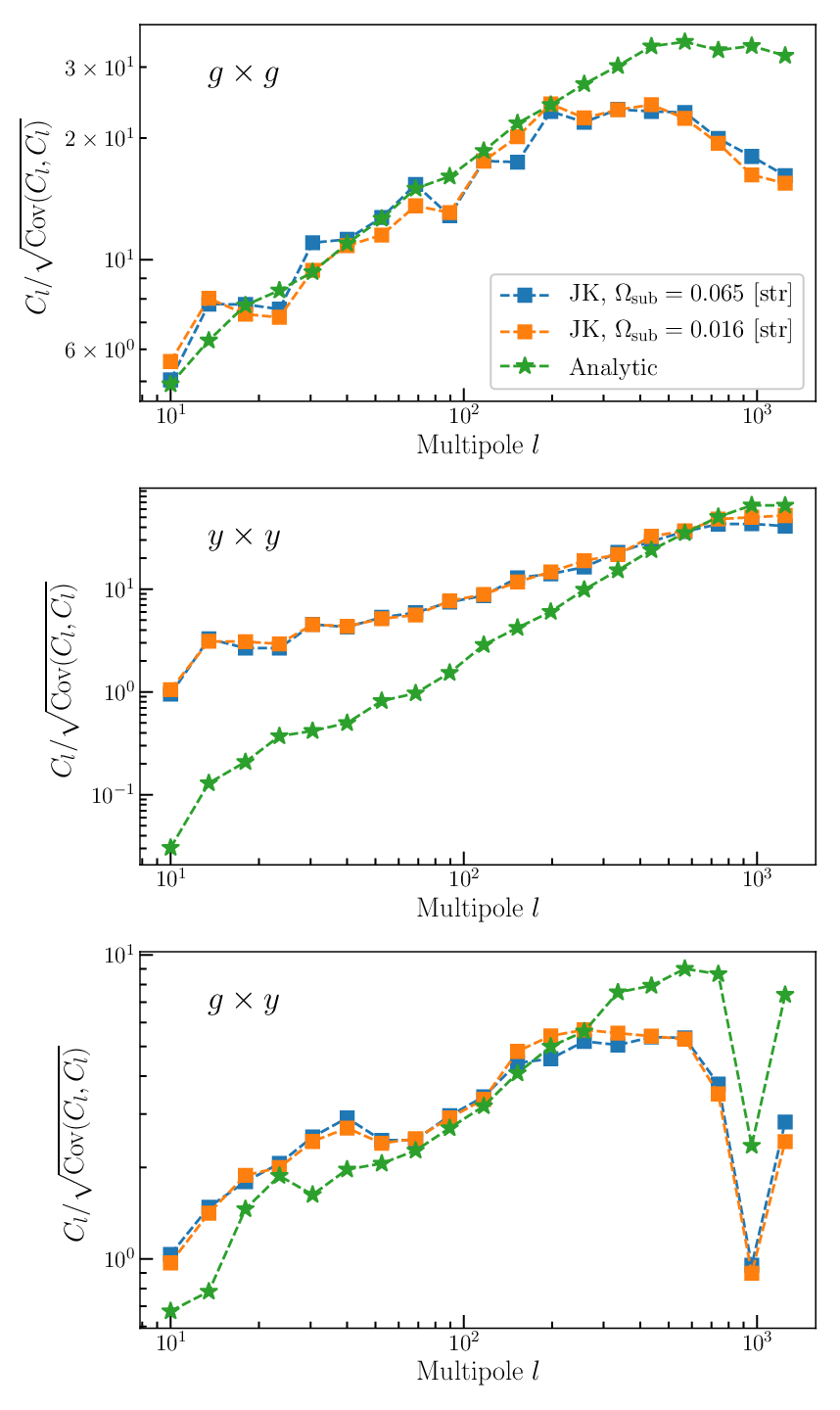
In Section 4 we used a covariance matrix obtained by the analytic formula, eq.(27). In this section we compare it with the one obtained by the Jackknife (JK) technique.
In the JK approach, we first divide the sky map into subregions with roughly equal areas in the sky. Then the auto- and cross-power spectra, , are estimated while masking out the patch of the sky. The covariance matrix is estimated from these resampled power spectra as,
| (33) |
where is the mean of resampled power spectra.
We define the JK subregions by using the coarse HEALPix map. In some of these subregions a large fraction of the area is already masked out by the Galactic and point source mask, and therefore the resampled power spectra are almost identical to the one measured by using the whole region. Thus we decided not to use subregions which are masked larger than of the total area. We checked the effect of this threshold and found that it does not strongly affect the results.
In Figure 11 we compare the signal-to-noise ratio at each multipole with the analytic error and the JK error. For the JK error, we show two results with varying the size of subregions.
For the 2MRS auto-power spectrum, the analytic errors and the JK error are consistent at large scales, suggesting there is no unknown systematics which is not included in the analytic model. On the other hand, the analytic errors are larger than the JK errors by a factor of 2–3 at small scales. It might be due to the halo-exclusion and non-linear effects, which complicates the shot noise (Ando et al. 2018).
The analytic error for the tSZ-auto power spectrum is an order of magnitude higher than the JK errors at large scales. This difference is due to non-Gaussian cosmic variance which is encoded in the tri-spectrum term in eq.(27). On the other hand, the JK errors are estimated from a single realization and cosmic variance cannot be captured. The same trend is also seen in the tSZ-galaxy cross-power spectrum but to much lesser extent.
We also performed parameter fitting with the JK covariance matrix, with the same settings described in Section 4.2. For the base-line model (i.e., fixed and ), the mean and 1 error of mass bias is for the tSZ auto and for the all power spectra, respectively. They are in agreement with the results with analytic covariance, but with smaller error bars.
References
- Ando et al. (2018) Ando S., Benoit-Lévy A., Komatsu E., 2018, MNRAS, 473, 4318
- Andreon (2014) Andreon S., 2014, A&A, 570, L10
- Arnaud et al. (2010) Arnaud M., Pratt G. W., Piffaretti R., Böhringer H., Croston J. H., Pointecouteau E., 2010, A&A, 517, A92
- Bocquet et al. (2016) Bocquet S., Saro A., Dolag K., Mohr J. J., 2016, MNRAS, 456, 2361
- Bolliet et al. (2018) Bolliet B., Comis B., Komatsu E., Macías-Pérez J. F., 2018, MNRAS, 477, 4957
- Bryan & Norman (1998) Bryan G. L., Norman M. L., 1998, ApJ, 495, 80
- Dolag et al. (2016) Dolag K., Komatsu E., Sunyaev R., 2016, Mon. Not. Roy. Astron. Soc., 463, 1797
- Górski et al. (2005) Górski K. M., Hivon E., Banday A. J., Wandelt B. D., Hansen F. K., Reinecke M., Bartelmann M., 2005, ApJ, 622, 759
- Hajian et al. (2013) Hajian A., Battaglia N., Spergel D. N., Bond J. R., Pfrommer C., Sievers J. L., 2013, J. Cosmology Astropart. Phys., 11, 064
- Hill & Spergel (2014) Hill J. C., Spergel D. N., 2014, J. Cosmology Astropart. Phys., 2, 030
- Hivon et al. (2002) Hivon E., Górski K. M., Netterfield C. B., Crill B. P., Prunet S., Hansen F., 2002, ApJ, 567, 2
- Hoekstra et al. (2015) Hoekstra H., Herbonnet R., Muzzin A., Babul A., Mahdavi A., Viola M., Cacciato M., 2015, MNRAS, 449, 685
- Hojjati et al. (2017) Hojjati A., et al., 2017, MNRAS, 471, 1565
- Horowitz & Seljak (2017) Horowitz B., Seljak U., 2017, MNRAS, 469, 394
- Howlett et al. (2012) Howlett C., Lewis A., Hall A., Challinor A., 2012, JCAP, 1204, 027
- Hu & Jain (2004) Hu W., Jain B., 2004, Phys. Rev. D, 70, 043009
- Hu & Kravtsov (2003) Hu W., Kravtsov A. V., 2003, ApJ, 584, 702
- Huchra et al. (2012) Huchra J. P., et al., 2012, ApJS, 199, 26
- Hurier & Lacasa (2017) Hurier G., Lacasa F., 2017, A&A, 604, A71
- Kay et al. (2004) Kay S. T., Thomas P. A., Jenkins A., Pearce F. R., 2004, MNRAS, 355, 1091
- Komatsu & Kitayama (1999) Komatsu E., Kitayama T., 1999, ApJ, 526, L1
- Komatsu & Seljak (2002) Komatsu E., Seljak U., 2002, MNRAS, 336, 1256
- Lau et al. (2009) Lau E. T., Kravtsov A. V., Nagai D., 2009, ApJ, 705, 1129
- Lavaux & Hudson (2011) Lavaux G., Hudson M. J., 2011, MNRAS, 416, 2840
- Lewis & Bridle (2002) Lewis A., Bridle S., 2002, Phys. Rev., D66, 103511
- Lewis et al. (2000) Lewis A., Challinor A., Lasenby A., 2000, Astrophys. J., 538, 473
- Ma et al. (2015) Ma Y.-Z., Van Waerbeke L., Hinshaw G., Hojjati A., Scott D., Zuntz J., 2015, J. Cosmology Astropart. Phys., 9, 046
- Medezinski et al. (2018) Medezinski E., et al., 2018, PASJ, 70, S28
- Meneghetti et al. (2010) Meneghetti M., Rasia E., Merten J., Bellagamba F., Ettori S., Mazzotta P., Dolag K., Marri S., 2010, A&A, 514, A93
- Nagai et al. (2007a) Nagai D., Vikhlinin A., Kravtsov A. V., 2007a, ApJ, 655, 98
- Nagai et al. (2007b) Nagai D., Kravtsov A. V., Vikhlinin A., 2007b, ApJ, 668, 1
- Navarro et al. (1997) Navarro J. F., Frenk C. S., White S. D. M., 1997, ApJ, 490, 493
- Osato et al. (2018) Osato K., Flender S., Nagai D., Shirasaki M., Yoshida N., 2018, MNRAS, 475, 532
- Page et al. (2007) Page L., et al., 2007, ApJS, 170, 335
- Penna-Lima et al. (2017) Penna-Lima M., Bartlett J. G., Rozo E., Melin J.-B., Merten J., Evrard A. E., Postman M., Rykoff E., 2017, A&A, 604, A89
- Piffaretti & Valdarnini (2008) Piffaretti R., Valdarnini R., 2008, A&A, 491, 71
- Planck Collaboration et al. (2013) Planck Collaboration et al., 2013, A&A, 550, A131
- Planck Collaboration et al. (2016a) Planck Collaboration et al., 2016a, A&A, 594, A13
- Planck Collaboration et al. (2016b) Planck Collaboration et al., 2016b, A&A, 594, A22
- Rasia et al. (2006) Rasia E., et al., 2006, MNRAS, 369, 2013
- Rasia et al. (2012) Rasia E., et al., 2012, New Journal of Physics, 14, 055018
- Salvati et al. (2018) Salvati L., Douspis M., Aghanim N., 2018, A&A, 614, A13
- Sánchez-Conde & Prada (2014) Sánchez-Conde M. A., Prada F., 2014, MNRAS, 442, 2271
- Schellenberger et al. (2015) Schellenberger G., Reiprich T. H., Lovisari L., Nevalainen J., David L., 2015, A&A, 575, A30
- Seljak (2000) Seljak U., 2000, MNRAS, 318, 203
- Sereno & Ettori (2017) Sereno M., Ettori S., 2017, MNRAS, 468, 3322
- Sereno et al. (2017) Sereno M., Covone G., Izzo L., Ettori S., Coupon J., Lieu M., 2017, MNRAS, 472, 1946
- Shi & Komatsu (2014) Shi X., Komatsu E., 2014, MNRAS, 442, 521
- Shi et al. (2015) Shi X., Komatsu E., Nelson K., Nagai D., 2015, MNRAS, 448, 1020
- Shi et al. (2016) Shi X., Komatsu E., Nagai D., Lau E. T., 2016, MNRAS, 455, 2936
- Skrutskie et al. (2006) Skrutskie M. F., et al., 2006, AJ, 131, 1163
- Smith et al. (2016) Smith G. P., et al., 2016, MNRAS, 456, L74
- Sunyaev & Zeldovich (1972) Sunyaev R. A., Zeldovich Ya. B., 1972, Comments Astrophys. Space Phys., 4, 173
- Tinker et al. (2010) Tinker J. L., Robertson B. E., Kravtsov A. V., Klypin A., Warren M. S., Yepes G., Gottlöber S., 2010, ApJ, 724, 878
- Van Waerbeke et al. (2014) Van Waerbeke L., Hinshaw G., Murray N., 2014, Phys. Rev. D, 89, 023508
- Vikram et al. (2017) Vikram V., Lidz A., Jain B., 2017, MNRAS, 467, 2315
- Wang et al. (2014) Wang H., Mo H. J., Yang X., Jing Y. P., Lin W. P., 2014, ApJ, 794, 94
- Zheng et al. (2005) Zheng Z., et al., 2005, ApJ, 633, 791
- von der Linden et al. (2014) von der Linden A., et al., 2014, MNRAS, 443, 1973