General purpose ray-tracing and polarized radiative transfer in General Relativity
Abstract
Ray-tracing is a central tool for constructing mock observations of compact object emission and for comparing physical emission models with observations. We present Arcmancer, a publicly available general ray-tracing and tensor algebra library, written in C++ and providing a Python interface. Arcmancer supports Riemannian and semi-Riemannian spaces of any dimension and metric, and has novel features such as support for multiple simultaneous coordinate charts, embedded geometric shapes, local coordinate systems and automatic parallel propagation. The Arcmancer interface is extensively documented and user-friendly. While these capabilities make the library well suited for a large variety of problems in numerical geometry, the main focus of this paper is in general relativistic polarized radiative transfer. The accuracy of the code is demonstrated in several code tests and in a comparison with grtrans, an existing ray-tracing code. We then use the library in several scenarios as a way to showcase the wide applicability of the code. We study a thin variable-geometry accretion disk model, and find that polarization carries information of the inner disk opening angle. Next, we study rotating neutron stars and determine that to obtain polarized light curves at better than level of accuracy, the rotation needs to be taken into account both in the space-time metric as well as in the shape of the star. Finally, we investigate the observational signatures of an accreting black hole lensed by an orbiting black hole. We find that these systems exhibit a characteristic asymmetric twin-peak profile both in flux and polarization properties.
Keywords:
methods: numerical — gravitation — gravitational lensing: strong — radiative transfer — polarization — accretion, accretion disksI Introduction
Fully covariant radiative transfer in General Relativity (GR) presents distinct complications. Due to gravity, the path of a wave front of radiation is curved even in vacuum. This leads to gravitational lensing, which causes measurable effects all the way from the scales of the Cosmic Microwave Background [126] and galaxy clusters [116] to Supermassive Black Holes (SMBHs) in centers of galaxies [73], down to single neutron stars [90]. Similarly, the rotation of the space-time itself, such as around rotating Kerr black holes, can cause an observable rotation of the direction of polarization of light. This phenomenon is known as (gravitational) Faraday rotation [110, 28, 57]. Finally, the observed intensity is also dependent on the relative position and velocity of the observer with respect to the elements of the emitting, absorbing and scattering medium – typically an astrophysical plasma – through which the light has propagated [44, e.g.]. This dependence is responsible for such effects as the Doppler (de-)boosting, via velocities of the emitter and observer, and gravitational and cosmological redshifts, via relative positions in the space-time, respectively.
A full (classical) solution of the polarized radiative transfer problem in GR requires solving the Einstein field equations, the magnetohydrodynamic equations of motion of the radiating and interacting matter, and the curved-space Maxwell equations simultaneously. This is a formidable undertaking, also in terms of computational resources, and significant progress has been made only relatively lately [see 62, and the references therein]. The problem becomes less taxing by assuming that the radiation field makes a negligible contribution to both the space-time curvature and the motion of the interacting medium. In this case, the underlying space-time structure and the state of the interacting medium can either be specified by analytic means, or by a separate numerical computation. However, even in this case, the full curved-space Maxwell equations need to be solved in the entire computational domain, which is still a computationally demanding task.
The situation is considerably simplified by the fact that the exact time-dependent behaviour of the electromagnetic and fields is not usually required, and knowledge of the radiative energy flow, i.e. specific intensity, is enough. In this case, it suffices to solve the usual radiative transfer equation, while taking into account General Relativity. There are numerous approaches with different limitations to solving the radiative transfer equation, such as Monte Carlo (MC) methods or the method of characteristics [see e.g. baron2004, and the references therein]. One of the perhaps conceptually simplest approaches is to use ray-tracing. In ray-tracing a mock observation can be constructed by connecting the observer to the emitting region through null geodesics (when plasma effects are unimportant, otherwise see e.g. gedalin2001 and Broderick & Blandford 13), through either analytic or numerical means. The bending of these geodesics captures the lensing effects of the gravitational field. The relativistic polarized radiative transfer equation can then be solved along these geodesics to capture the remaining relativistic effects. This process, called ray-tracing, is computationally efficient and naively parallelizable, enabling high resolution mock observations to be computed in seconds or minutes on a standard desktop computer. However, straightforward ray-tracing methods are limited to problems where scattering is not dominant. This is due to the fact that strong scattering couples all directions and spatial locations of the solution, whereas simple ray-tracing only samples the rays reaching the observer. In addition, if the radiative eigenmodes propagate differently due to strong plasma effects, then all eigenmodes must be propagated separately and similarly radiative transfer must be computed multiple times, increasing the workload considerably.
Despite these limitations, using ray-tracing to compute mock observations of highly relativistic objects has a relatively long history. Already in Cunningham & Bardeen [32], the light curve of a star orbiting around a black hole was computed, followed by studies of the effects of gravity on the observed accretion disk spectra [31, 30]. Polarization effects of relativistic motion and strong gravity in the Kerr solution were studied using ray-tracing in Stark & Connors [110], Connors & Stark [28] and Connors et al. [29]. The first resolved mock observation of an accretion flow around a black hole was computed via ray-tracing remarkably early as well, in Luminet [73]. Following these pioneering studies, the ray-tracing approach was quickly adopted to investigations of a great variety of relativistic phenomena, including but not limited to: hot spots and accretion columns on rotating neutron stars [90, 101], the general mock observation problem in the Kerr space-time [120], details of the resolved black hole accretion disk structure [43, 17], accretion disk hot spots [60], accretion disk microlensing [99, 59], accretion disk line profiles [26, 40], optical caustics [100] and the shadow cast by the black hole event horizon [42].
In particular, the topics of the black hole shadow and accretion flow as well as the observable polarization properties of neutron stars are currently especially relevant. The interest in black hole shadows and accretion flows is warranted by the recent progress in programs for interferometric observations at the event horizon scales of Sgr A∗, the Milky Way supermassive black hole, and the SMBH in M87, the dominant galaxy of the Virgo cluster. The event horizon is approached both in the sub-mm wavelengths, via the Event Horizon Telescope (EHT) VLBI program [38], and in optical wavelengths via the VLTI GRAVITY instrument [41]. The surging interest is evident also in the number of recent studies focusing on the black hole shadow and accretion flow modeling using ray-tracing, especially in the context of Sgr A∗ [36, 46, 16, 4, 21, 123, 49, 94, 81, e.g.].
Likewise, accurate modeling of the observable properties of neutron stars is timely due to the current and near-future increase in X-ray sensitive space missions such as NICER [47] and eXTP [128], of which the latter is also sensitive to polarization. In anticipation, a number of recent papers have applied the ray-tracing approach to model observations of neutron stars [7, 8, 78, 72, 50, 35, 83, 125, e.g.].
It is evident even from the short review above that ray-tracing is an important numerical tool, especially for general relativistic radiative transfer in a variety of astrophysical situations. However, the numerical means to compute curves has an even wider applicability in the sense that in addition to the path of light, curves also represent the timelines of massive particles and observers in a space-time. Furthermore, it is often convenient to have various tensorial quantities such as local Lorentz frames parallel transported (or more generally, Fermi–Walker transported) along curves. It is also necessary to perform various algebraic computations involving tensor quantities, often mixing different coordinate systems.
To help facilitate numerical studies requiring curve and tensor manipulations in any (Semi-)Riemannian context, which naturally includes GR, we have implemented Arcmancer [code_zenodo]11 1 Codebase: https://bitbucket.org/popiha/arcmancer, a publicly available general ray-tracing and tensor algebra library. From an astrophysical point of view, Arcmancer is useful for such varied tasks as radiative transfer and mock observations, computing the paths of massive charged particles in curved space-times or calculating the orbits of extreme mass-ratio inspirals (EMRIs). However, the Arcmancer library offers capabilities beyond purely physically motivated applications. It can compute all kinds of curves, both geodesic and externally forced, on Riemannian and semi-Riemannian manifolds of any dimension and metric, using multiple simultaneously defined coordinate charts to circumnavigate coordinate singularities and to facilitate easy input and output of data in any preferred coordinate system. Arcmancer can also be used to define tensors of any rank, and to perform tensor algebra, as well as for example automatically parallel propagate tensorial quantities along curves. This last feature is particularly useful for problems of radiative transfer, on which we will mainly focus in this paper.
In this paper, we present an overview of the Arcmancer library and its implementation. We show the results of various code tests to establish the accuracy of the code, and present several astrophysical applications using the Arcmancer library. In this paper, the main focus of the tests and applications is in general relativistic polarized radiative transfer using ray-tracing exclusively. The generality of the Arcmancer library makes it straightforward to use for more general purpose radiative transfer methods such as Monte Carlo (MC) radiative transfer or hybrid MC–ray-tracing schemes, and the application of these will be demonstrated in future works. The paper is organized as follows. In Section II we present an overview of the Arcmancer library and its capabilities. In Section III we discuss how the various mathematical objects and functionalities provided by the Arcmancer library are implemented. For convenience, these differential geometric concepts are briefly reviewed in Appendix A, to which Section III cross-references to. Section IV describes the implementation details of the radiative transfer scheme implemented in Arcmancer. In Section V, we present a series of numerical tests, measuring the accuracy of the numerics implemented in Arcmancer. These include a test of the radiative transfer features, where the results obtained with Arcmancer are compared to another recent general relativistic code grtrans [36]. In Section VI, the Arcmancer code is applied to various astrophysical phenomena in order to showcase the versatility of the code. Finally, in Section VII we give concluding remarks, and discuss some future prospects concerning the Arcmancer library and the ray-tracing approach in astrophysics. The paper comes with several Appendixes. Appendix A presents a highly condensed review of the various differential geometric concepts used in the code. Appendix B presents the general relativistic polarized radiative transfer equation used in Arcmancer, and how it relates to the usual flat-space equation. Appendix C presents the built-in manifolds and coordinate systems available in Arcmancer.
The reader interested mainly in a broad overview of the code and its astrophysical applications is urged to browse Sections II, V.2.2 and VI. Those interested in technical details may want to read through Sections III, IV and V, and the Appendixes as well.
Throughout the paper, we use a system of units where , unless explicitly otherwise specified. For Lorentzian space-times, we use a metric signature in the paper, although Arcmancer supports other signatures as well. The abstract index notation (see Appendix A.2) is assumed throughout.
II Overview of the code
The Arcmancer library consists of a core library, written in modern C++, a Python interface and a suite of example C++-programs and Python scripts. The core library code, Python interface and example programs are all thoroughly documented. The code, the examples and instructions for installation and getting started are all freely available at the code repository, https://bitbucket.org/popiha/arcmancer.22 2 The version of the code used to produce the results in this paper is version 0.2.0, which corresponds to the commit identifier 38b0879909990746f28e09fb1f94167063608be9 at the master branch of the repository.
The underlying idea behind the Arcmancer library is to provide all the mathematical tools needed to perform a large variety of relativistic computations that require numerical tensor algebra and curve propagation. In addition, the library and the Python interface are designed with easy extensibility in mind. These design decisions make it possible to use Arcmancer for a wide variety of astrophysical problems, including for example particle dynamics and radiative transfer, as well as for problems in applied mathematics.
These design goals give Arcmancer some distinct advantages compared to existing ‘pure’ ray-tracing codes such as grtrans [36], GYOTO [124], KERTAP [25], GRay [23, 22] or ASTRORAY [108]. Namely, Arcmancer can work in any dimension and with metric spaces that are either Lorentzian, as in GR, or purely Riemannian. For Lorentzian geometry, all types of geodesics – null, spacelike and timelike – are supported, as well as general curves of indeterminate classification. Arcmancer can also work with spaces for which the geometry, through the metric, is available only numerically, such as from a numerical relativity simulation. In addition, Arcmancer supports any number of simultaneous coordinate systems with automatic conversion of all quantities between coordinate systems. The use of multiple coordinate systems makes it possible to input and output data in whatever coordinates are most convenient for the given problem. Furthermore, simultaneous use of multiple coordinates makes it possible for Arcmancer to avoid coordinate singularities, and to automatically choose the numerically most optimal coordinate system for propagating a curve (see Section III.5).
Arcmancer provides full support for tensorial quantities of any contra- or covariant rank (see Section III.2). This support is built on top of the Eigen Linear Algebra Library and includes all the usual tensor operations such as sums, products, contractions of indices and raising and lowering of indices with the metric. All these operations are checked at compile-time so that mathematically malformed operations, such as mixing points and vectors or contracting two similar indices are automatically detected. In addition, Arcmancer can automatically parallel transport all tensor quantities along curves, so that e.g. smooth local coordinates can be constructed for an observer undergoing arbitrary geodesic motion. This functionality also supports Fermi–Walker transport for accelerating observers, and fully general transport for e.g. accelerating and rotating observers.
Arcmancer also provides support for including user-defined embedded geometry (see Section III.4). This feature can be used, for example, to model surfaces of optically thick or solid astrophysical objects, such as planets, photospheres of stars or neutron stars or optically thick accretion disks. The surfaces are easy to define through level sets, and can be given tangential vector fields, which represent movement along the surface, such as in the case of a rotating surface of a neutron star or an optically thick accretion disk.
Finally, while Arcmancer comes with a suite of built-in space-times, coordinates, geometries, and radiation models, the library is designed to be easily extensible by the user. Several examples showcasing this easy extensibility are bundled together with the Arcmancer library. These examples include such programs as simple black hole and neutron star imagers, as well as a full postprocessor for two-dimensional data produced by the GR magnetohydrodynamics (GRMHD) code HARM [45, 84].
In the following, we will discuss in more detail how the C++ library implements the mathematical concepts required for the wide variety of applications described above.
III Implementation of differential geometry and ray-tracing
The main aim of the Arcmancer implementation is to provide the user with C++/Python objects that match the mathematical objects of differential geometry (see Appendix A) as closely as possible. This approach makes converting mathematical formulae to code straightforward. It also has the additional benefit of eliminating errors stemming from code that expresses mathematically invalid operations. These include, for example, assigning to the components of a point from the components of a vector or a one-form, since all can be expressed as a tuple of numbers, or assigning to the components of a vector from the components of a vector defined at a different point, in a different chart, or even defined on a different manifold. Likewise, for tensorial quantities, an error such as contracting two similar indices is easily made if working in terms of pure components.
The implementation in Arcmancer guarantees that all programmed operations correspond to mathematically valid statements. This feature eliminates a large set of logical errors of the kind described above – a major benefit, since currently there are no codebase analysis tools able to identify errors of this kind.
In the following, we describe how the mathematical objects are implemented in the Arcmancer code. To make the exposition easier to follow, we have provided a list of the most important C++ classes of the Arcmancer library together with their descriptions in Figure 1. The Python interface provides corresponding counterparts to these classes, together with some additional convenience classes. A listing of these can be found in the documentation accompanying the code.
III.1 Manifolds and charts
The most fundamental object in the Arcmancer library is MetricSpace<n,Signature>, representing an -dimensional (semi-)Riemannian manifold of a given signature. Defining a new MetricSpace requires the specification of dimensionality , one or more charts, and functions returning the components of the metric tensor field and its derivatives in each chart. For four-dimensional semi-Riemannian spaces, the metric signature must also be specified. Arcmancer supports both timelike and spacelike signatures.
A chart is represented as a class Chart that in the current implementation only contains a description and serves to give meaning to a tuple of coordinate numbers. The points on the manifold are implemented as a class ManifoldPoint<MetricSpace>. These can be constructed by specifying coordinates and the corresponding chart. After this, the components of the point can be requested in any available chart, and the object itself behaves much like the mathematical idea of a point on a manifold (see Appendix A.1).
For transforming the components of tensorial objects, the transition functions and their Jacobians between the charts must also be specified. For different charts this would naively require transition functions and Jacobians to be implemented. The amount of work increases quadratically. However, when the domains of charts , and overlap suitably, the transition function from -coordinates to -coordinates fulfills
| (1) |
and the Jacobian decomposes similarly,
| (2) |
The Arcmancer library uses the properties (1) and (2) to build a directed graph of charts, wherein each chart is a node, and the Jacobians and transition functions define the edges. This makes it possible to introduce charts while supplying only the minimum number of transition functions and Jacobians to make the graph connected. Then, when the components of a point or a tensorial quantity are requested in a different chart, the code walks through the graph building the transition function and Jacobian piece by piece using equations (1) and (2).
For a listing of the built-in metric spaces and chart implementations provided with Arcmancer, see Appendix C.
III.2 Tensors
Tensor algebra and calculus for tensors of arbitrary rank (see Appendix A.2) is provided by the Tensor<MetricSpace,Indices...> template class. Here MetricSpace is the base manifold and Indices... is an arbitrary combination of index tags Cov and Cnt, for covariant or contravariant index, respectively. The implementation is pointwise, using a set of components in a given chart to specify a tensor of rank on a manifold with at a given ManifoldPoint.
As such, similarly to a ManifoldPoint, defining a tensor at a point requires the input of components and the corresponding chart. After this, the chart is abstracted away in the sense that algebraic operations between tensors defined at the same point can be performed irrespective of the chart the tensors were originally defined in. The Tensor class provides all the usual algebraic tensor operations: sum of tensors of same rank, tensor product, contraction and additionally raising and lowering of the indices using the underlying MetricSpace structure. The implementation checks all operations for index correctness at compile time, so that e.g. no contraction between indexes of same type is allowed. In addition, during runtime, all operands are inspected to ensure that they are defined at the same base point. These checks guarantee that operations expressed in code correspond to mathematical operations that are well defined.
The Tensor class also provides some elements of tensor calculus. Namely, the class automatically computes the derivatives required for parallel transporting a tensor along a general curve. Given a curve tangent vector , the class can compute the contractions with required in the parallel transport equation (A9).
III.3 Curves
Functionality for working with curves , including geodesics, is provided by the class ParametrizedCurve<MetricSpace,TransportedType> along with a convenience subclass Geodesic. Curves are implemented as sequences of points on a manifold, where is the curve parameter and . More concretely, the implementation is based on an ordered queue of objects of type ParametrizedPoint<MetricSpace,TransportedType>, which combine a ManifoldPoint with a real value specifying the position along the curve. In addition, the ParametrizedPoint can include any arbitrary object of type TransportedType to be parallel transported along a geodesic or, for example, Fermi–Walker transported along a forced curve. The only requirement is that the object be representable as a (chart-dependent) tuple of real numbers, and that a function yielding the derivatives is provided. The function depends externally on the current tangent vector of the curve , the contractions and optionally the force . As mentioned above, Tensor class provides the derivative function automatically, and as such arbitrary tensors can be parallel transported along all generic curves without any extra programming effort.
In practice, a curve is computed by specifying the initial conditions in some given chart. These consist of the initial point , the components of the curve tangent vector , the components of the possible parallel transported object, and an optional force function . The Arcmancer library then computes points along the curve for the desired interval containing by solving the set of equations (see Appendix A.4)
| (3) | ||||
| (4) | ||||
| (5) |
in a suitable chart (see Section III.5 for details on the chart selection).
Arcmancer computes the solution using the integration methods offered by the Odeint C++ library [1]. The default method is the Dormand–Prince 5th order Runge–Kutta method [39], which offers error estimation and automatic stepsize adjustment, as well as a fair numerical performance in most cases. The absolute and relative error tolerances and stepsize and iteration limits are fully user-configurable. After the computation is finished, the ParametrizedCurve class provides access to the solution in any chart and for any . Internally this is achieved through a cubic spline interpolation.
III.4 Surfaces
An interface for implementing hypersurfaces is available through the class Surface<MetricSpace>. Surfaces are useful for representing solid or highly optically thick objects, or regions of interest. Examples include the surfaces of neutron stars, white dwarfs or planets but also black hole event horizons, optically thick accretion disks or the limits of computational domains. The Arcmancer implementation of surfaces is based on the concept of level hypersurfaces (see Appendix A.5).
A new surface is implemented by supplying a real valued function taking a ManifoldPoint as an argument, as well as the gradient . The surface is then defined as the set of points . In addition, a tangent vector field on the surface must be defined. This field is primarily used to represent the four-velocity field of observers fixed on the surface, and is required for e.g. computations involving rotating neutron stars (see Section VI.2).
The Arcmancer library automatically detects intersections of curves with surfaces, and numerically finds the exact (to within tolerance) intersection point. The intersections are found by examining the sign of the product for two successive points and on a curve. If the product is negative, the two points must lie in different regions bounded by the surface. The exact intersection point is then found using the so-called Hénon’s trick [54]. The ‘trick’ consists of changing the independent variable , the curve parameter, in equations (3)–(4) to , or the value of the surface function. The transformed equations read
| (6) | ||||
| (7) | ||||
| (8) | ||||
| (9) |
These equations can then be numerically propagated for a single step of length starting from the point to yield the intersection point to within numerical tolerance.
III.5 Automatic chart selection
Perhaps the most novel and interesting feature of Arcmancer is the possibility to use multiple coordinate charts simultaneously and seamlessly. The most immediate benefit is that objects can be input and output in any available chart, with all transformations handled automatically by Arcmancer. However, there are important computational benefits to free selection of coordinate charts as well. The most obvious benefit is the fact that a given problem may be much easier to solve numerically in some specific coordinates compared to others. This is illustrated in Figure 2, where the same null geodesic in an extremal Kerr space-time is shown in the outgoing Kerr–Schild coordinates, the ingoing Kerr–Schild coordinates and the Boyer–Lindquist coordinates (see Appendix C.2.2). From the figure, it is easy to appreciate how in the outgoing Kerr–Schild coordinates the geodesic is essentially straight, and long integration steps can be taken. On the other hand, in the ingoing Kerr–Schild coordinates and the Boyer-Lindquist coordinates the geodesic twists around the event horizon at an increasing rate as the event horizon is approached. The magnitudes of the derivatives with respect to the curve parameter increase correspondingly, making the problem eventually numerically impossible to solve.
The possibility to simultaneously use multiple charts makes it possible to avoid the coordinate singularities present in any single chart, such as the pole singularity in any spherical coordinate system, or the coordinate singularity at the event horizon present in the usual Schwarzschild coordinates. In addition, using multiple charts makes it possible to switch the chart used for solving the equations of motion for a curve on the fly, useful for situations such as the one depicted in Figure 2. It is not obvious which chart is to be preferred, which is why Arcmancer currently implements several heuristics for automatically choosing the numerically optimal chart.
The first heuristic consists of finding a chart where the matrix of the components of the metric has the largest inverse condition number, defined as the ratio of the smallest and largest singular value of the matrix, i.e. . This is based on two key observations. Firstly, floating point addition and substraction between numbers of different magnitude causes a loss of precision. Secondly, the equations of motion for a curve and for parallel transport along it, (3)–(5), contain a mix of the components of the metric and its derivatives on the right-hand side. As such, it would be intuitively advantageous to perform the computations in a chart where the matrix formed by the metric has eigenvalues that span as small a range as possible. This is achieved by maximizing the inverse condition number.
In some cases the condition number of the metric is not enough to detect a computationally awkward chart. For example, in the case of a Kerr black hole, the condition number cannot differentiate between the ingoing and outgoing Kerr–Schild charts. However, as is seen in Section V.1.2, using one over the other can cause a large difference in computation time and accuracy for radial geodesics, depending on whether they are falling towards or emanating from the event horizon. As such, a further heuristic is needed.
If the condition number heuristic does not separate two promising charts, the Arcmancer code next tries to minimize the maximal absolute value of the intrinsic derivatives, , of the curve tangent vector . As such, this heuristic needs to know the current curve tangent vector , unlike the condition number test, for which only the current point is required. For Cartesian coordinates in a Euclidean or Minkowskian space , so in effect this procedure looks for the most Cartesian-like chart in which the metric looks most Euclidean (or Minkowskian) in the direction of the current curve tangent vector .
Formal proofs of the performance of these heuristics are beyond the scope of this work, but the numerical results in Section V indicate that they work reasonably well.
III.6 Local Lorentz frames
For four-dimensional Lorentzian manifolds, Arcmancer provides a functionality to construct local Lorentz frames (see Appendix A.6) through the class LorentzFrame<MetricSpace>. The user supplies a timelike vector and two spacelike vectors and . From these, a complete Lorentz frame is constructed by first normalizing to yield and then orthonormalizing and sequentially. Finally, is defined by the remaining orthogonal direction through , where is the Levi–Civita tensor, with sign depending on the desired handedness (positive for a right-handed frame).
The LorentzFrame object can be automatically parallel transported along a ParametrizedCurve. In addition, Tensor objects can be constructed from components given with respect to a LorentzFrame. Likewise, the components of any Tensor can be extracted in a given LorentzFrame as well, see equation (A11).
III.7 Image plane generation
To produce mock observations, an observational instrument must be emulated somehow. For ray-tracing purposes, this usually means using an image plane. The image plane is positioned near the object of interest, and only the rays intersecting the plane orthogonally are considered. These rays are then assumed to propagate in vacuum all the way to the distant observer. This approximation neglects atmospheric and instrumental effects, but these can be modeled afterwards using dedicated tools if necessary.
There are three main sources of error when generating the image plane: required deviations from perpendicularity, perturbations caused by the curvature of the space and the assumption of vacuum propagation. The assumption of perpendicularity is typically excellent. For distant objects, the maximum deviation from perpendicularity is approximately equal to the observed angular size of the object, or , where is the linear extent of the source perpendicular to the line of sight and the distance. For example, in the case of Sgr A∗ (Sagittarius A∗), we have , and for a typical galactic neutron star . The effects of remaining space-time curvature at the image plane location can be estimated by looking at the bending angle that the image plane rays will make when propagated to infinity. Sufficiently far away from the object so that the Schwarzschild metric can be used, this angle turns out to be [10, e.g.] , where is the total mass of the observed object and is the radial distance of the image plane from the object. Thus, for we have , and so the effects of residual curvature are negligible. The assumption of propagation in vacuum is typically valid for objects that are not situated at cosmological distances as far as the light bending is concerned. However, corrections for effects such as extinction, frequency dispersion or Faraday rotation may need to be added in further postprocessing.
In many ray-tracing codes, the construction of image planes is achieved by a assuming a flat space and explicitly constructing the starting points and tangent vectors for a planar configuration of geodesics [15, 19, 37, 124, 36, 22]. Arcmancer provides a general-purpose tool for constructing plane-parallel initial conditions for Lorentzian space-times in class ImagePlane<MetricSpace,DataType>. The user specifies a LorentzFrame at the center of the plane and the extent and the resolution (number of grid points) of the plane in the local and directions. The local Lorentz frame is then parallel transported to the desired grid points via spacelike geodesics, using the Arcmancer curve propagation functionality. Initial conditions for curves passing through the plane are set up by assigning the tangent vectors to be spatially parallel to the parallel transported vector. The collection of parallel transported frames defines a best local approximation to a flat plane that is threaded by orthogonal curves, and corrects the effect of the bending caused by the curvature to first order. Thus, the Arcmancer ImagePlane can safely be used in regions where the curvature is small but non-negligible. The method is also general purpose in the sense that it works similarly in any coordinate system and only requires specifying a local Lorentz frame at one point.
IV Implementation of radiative transfer
IV.1 Fluid and radiation models
Radiative transfer functionality in Arcmancer is built with flexibility in mind. For this purpose, the interface declares two types of functions. The first type is a FluidFunction<MetricSpace,FluidData> which maps points on the base manifold MetricSpace to a user-defined set of fluid variables FluidData, which represent local material properties such as temperature or density. The only restriction is that FluidData must include a single bulk fluid four-velocity and a single reference direction (often magnetic field) orthogonal to .
The second type of function is RadiationFunction<FluidData>, which computes the Stokes emissivity vector and the response matrix (see Appendix B) from the given FluidData, local fluid rest frame frequency , and the rest frame angle between the reference direction and the current direction of the light ray (the tangent vector ).
This approach makes implementing different fluid and radiation models rather straightforward. For example, the fluid variables for a given point can be obtained from a GR magnetohydrodynamics (GRMHD) simulation or from an analytic model. The Arcmancer suite includes an example application which reads outputs from the HARM GRMHD code [45, 84] and computes mock observations using a thermal synchrotron radiation model based on the results in Dexter [36]. See Section V.2.2 for computational results.
IV.2 Solving the radiative transfer equation
With Arcmancer, a radiative transfer problem (see Appendix B) is solved by first propagating a set of curves (typically geodesics, unless plasma effects are significant) along which the radiative transfer equation, eq. (B7), is to be solved as a curve integral. Usually, the most convenient approach is to use an ImagePlane and let Arcmancer propagate the set of initial conditions backwards in time through the region of interest. Each propagated curve must include a parallel transported PolarizationFrame, a pair of two orthogonal spacelike vectors , also orthogonal to the geodesic and the four-velocity of the observer, representing the vertical and horizontal linear polarization basis vectors of the observer at one end of the curve. If using an ImagePlane, these can be conveniently obtained from the and vectors of the local Lorentz frame at each point.
The four-velocity of the observer at , the four-velocity of the fluid at each point and the curve tangents and define a connection between the photon frequency observed by at and the corresponding photon frequency in the local rest frame of the fluid at . This is given by the redshift factor
| (10) |
The initial conditions are set by defining initial invariant specific intensities at the other end of the curve, one for each observed frequency of interest. Often these can be set to zero, but for example in the case of radiation emanating from optically thick or solid surfaces, the initial intensity can be non-zero. Solving the radiative transfer equation itself proceeds in a manner following [107]. See Figure 3 for a diagram of all the vectors and angles.
At each point during the calculation, the Arcmancer library evaluates the given FluidFunction to obtain the fluid four-velocity and the rest of the fluid parameters in the rest frame of the fluid. This includes the local reference direction , which typically is the direction of the local magnetic field. From these, the angle between the reference direction and the light ray tangent as seen in the fluid rest frame is computed using equation (A15). This angle is required by some radiation models, such as synchrotron emission models. The reference direction also defines the local vertical direction of polarization , where and are the spatial parts of and , respectively.
The next step is to project the parallel transported polarization frame to the fluid rest frame using the screen projection operator, equation (A14), yielding , where
| (11) | ||||
| (12) |
Now we can compute the angle between the projected parallel transported polarization frame and the polarization frame of the fluid, defined by , from
| (13) |
where .
Next, the angle and the fluid parameters are passed to the RadiationFunction to obtain the Stokes emissivity and the response (Müller) matrix in the fluid rest frame. These are related to the parallel transported and projected polarization frame using the angle and the transformation properties of the Stokes components under rotation [24, e.g.]. The emissivity vector and response matrix are transformed via and , where
| (14) |
gives the transformation of Stokes vectors under rotations of the polarization plane. Finally, it can be shown that the Stokes components in any two polarization frames and related by a screen projection are equal, so that the radiative transfer equation to be solved along the geodesic is
| (15) |
where
| (16) | ||||
| (17) | ||||
| (18) |
and is the unit of length. For example, in problems related to black holes, a typical choice is , where is the black hole mass. Internally, equation (15) is solved using the Odeint Runge–Kutta–Fehlberg 8th-order method. However, for problems where the optical thickness is large, the equation (15) can become stiff, and an implicit method would provide better performance.
V Code tests
V.1 Curves, parallel transport and chart selection
V.1.1 Geodesic propagation
The accuracy of the basic curve propagation functionality (Section III.3) was verified by investigating curves on a two-dimensional spherical surface. The computations were performed both in two dimensions, using the intrinsic spherical coordinate chart , equation (C1), and in a three-dimensional Euclidean slice at of the Minkowski space using the spherical coordinates , equation (C3). To force the curve to stay on the surface of a sphere in the three-dimensional case, a constraint force was specified. Here is the curve tangent, in three-dimensional spherical coordinates.
Numerical convergence was estimated using a single geodesic curve passing through at with a tangent vector . The initial values were chosen so as to avoid a purely polar or equatorial geodesic, but were otherwise chosen arbitrarily. The geodesic was computed several times using a range of equal relative and absolute numerical tolerances and from to in 40 steps. The differences between the numerical results and the known analytical solution are shown in Figure 4. We see that both in the intrinsic two-dimensional and the constrained three-dimensional case the numerical curves converge towards the analytical solution linearly with the tolerance parameters. The convergence saturates at tolerance parameters when the relative precision floor of the double precision floating point numbers is reached.
V.1.2 Parallel propagation in the Kerr space-time
The functionality for parallel transporting tensorial quantities (see Sections III.2 & III.3) along a curve was assessed in the context of a Kerr space-time (see Section C.2.2) with a near-extremal non-dimensional spin parameter and mass . First, initial conditions and were fixed in the Boyer–Lindquist coordinates (see equation (C4)). These initial values were chosen to yield a generic timelike geodesic, and to avoid special cases such as equatorial geodesics, but were otherwise chosen arbitrarily. The geodesic was then augmented by including the metric and a Lorentz frame as quantities to be parallel transported. The geodesic was then computed until to yield several complete orbits around the black hole, using tolerances . Finally, the parallel transported values were evaluated for accuracy by comparing to analytic expectations.
Figure 5 shows the orbit of the geodesic. It also depicts magnitudes of the maximum difference of the components of the parallel transported metric with respect to the analytic expression, both computed in the ingoing Kerr–Schild chart. Also shown are the absolute values of all the pairwise inner products of the parallel propagated Lorentz frame which should be identically zero. From the figure we see that the errors in all of these conserved quantities increase in a secular fashion, while the single step errors are below the set numerical tolerance. This is an expected and well-known behavior for non-symplectic numerical integration methods, such as the 5th order Dormand–Prince scheme used in Arcmancer, which do not respect the geometric structure of the phase space [52]. Symplectic methods for the inseparable Hamiltonians occurring in geodesic propagation have been discovered recently [92], but these are not yet available in Odeint. In general, the secular accumulation of integration error poses no problem for the applications we demonstrate in this paper. However, for integrations over long periods of time, such as for computing dynamics of massive particles orbiting a black hole, a symplectic method for inseparable Hamiltonians might need to be implemented.
The accuracy and performance of both the curve propagation and parallel transport functionality was also assessed as a function of the geodesic and the coordinate chart. To this end, we set up an image plane at in the Boyer–Lindquist (BL) coordinates of a Kerr space-time with and . From the image plane, null geodesics were propagated backwards from to or until intersection with a surface slightly outside the event horizon, defined by , where is the event horizon radius. This radius was chosen since the computation in the Boyer–Lindquist and ingoing Kerr–Schild coordinates must be terminated before the event horizon itself (see Figure 2). The geodesics were computed three times, each time fixing the chart (automatic chart selection disabled) to either ingoing Kerr–Schild (KS), outgoing KS or the Boyer–Lindquist chart. Standard tolerances of were used. We then computed the maximal absolute errors in the value of the curve Hamiltonian, , and the trace of the parallel transported metric along the geodesics, and plotted these on the image plane, in addition to the number of integration steps . The results are shown in Figure 6.
From the figure, it is evident that the outgoing KS coordinates offer significantly better numerical performance than the ingoing KS coordinates or the BL coordinates. This is not surprising, since the outgoing KS chart is adapted to radially outgoing null geodesics. As a consequence, the more radial the geodesic is, the more nearly a straight line it is in the outgoing KS chart. In the figure, this can be seen as the remarkable decrease in the maximal error and the number of computational steps for the geodesics starting near the origin of the image plane (see also Figure 2). On the other hand, the BL coordinates are seen to perform significantly worse. This is related to both the fact that the geodesic ‘wraps around’ the black hole near the event horizon (see Figure 2), but also the fact that the condition number (the ratio of the maximum to minimum singular value) of the matrix of the metric components scales as (see Section III.5). In addition, the coordinates are singular at the poles. All these factors combine to make the BL chart the most numerically disadvantageous of the three. Finally, the ingoing KS chart fares worse than the BL chart for the conservation of the Hamiltonian, but better for the trace of the metric tensor and number of steps taken. This is understandable, since these coordinates are adapted to radially ingoing null geodesics, and outgoing geodesics ‘wrap around’ the black hole near the event horizon twice as fast compared to the BL coordinates. This is partly offset by the fact that the condition number of the metric components is better behaved than for the BL coordinates. The ‘wrap-around’ behavior is suppressed near the poles of the black hole, which in the figure can be seen as the slight decrease in the error of the metric trace around the ‘North’ pole of the black hole for the BL and the ingoing KS coordinates.
The accuracy in general is seen to be consistent with the given numerical tolerances. The outgoing KS chart in particular provides excellent accuracy, with results much better than even the set tolerances for nearly radial geodesics. In addition, there is a factor of difference in the number of steps taken between the outgoing KS chart and the BL chart, which was also directly reflected in the computational time. The results strongly suggest that the outgoing KS metric should be preferred in all codes computing mock observations using geodesics emanating from the vicinity of a Kerr black hole. Likewise, for studies of radiation scattering from a black hole, ingoing KS coordinates should be used for computing the incoming radiation and outgoing KS coordinates for the scattered, outgoing radiation.

V.2 Radiation tests
We assessed the accuracy and convergence properties of the Arcmancer radiative transfer functionality by postprocessing a general relativistic magnetohydrodynamics (GRMHD) simulation, and by comparing to an existing polarized radiative transfer code grtrans [36]. To facilitate an easy comparison, we used the same simulation data as was used to test grtrans, as the data is conveniently distributed with the grtrans code.33 3 The data is found in the file dump040, found online at https://github.com/jadexter/grtrans/blob/master/dump040. The simulation data used was computed with the GRMHD code HARM [45, 84], and describes an axisymmetric optically thin accretion flow around a Kerr black hole with a dimensionless angular momentum of . The black hole mass and its accretion rate were set to the grtrans defaults for HARM, and . Assuming in addition that the source is at a distance of , these values approximate Sgr A∗ [36], although for this particular data set at the observed frequency of the total computed flux of (see below) is roughly three times too large compared to the observed value of [11, e.g.]. The radiative model was taken to be relativistic thermal synchrotron radiation, using the updated formulae in Dexter [36]. The electron and proton temperatures in the plasma were assumed equal, and the ideal gas equation of state was assumed, also corresponding to grtrans.
All mock observations were computed using a square image plane with physical dimensions , where , in the local Lorentz frame of a stationary observer with (see Section III.6 and Appendix A.6.1). The negative -axis is pointed towards the origin of the Boyer-Lindquist (BL) coordinates. The image plane was set at a distance and an inclination of (in BL coordinates), as in Dexter [36]. Geodesics from the image plane were then computed backwards in time from the image plane and the radiative transfer computed at the observed frequency of along these geodesics to form the final image. Numerical tolerances for both the geodesic computation and the radiative transfer computation were set to . These tolerances guarantee that the accuracy during radiation transfer is governed by the chosen sampling rate , where is the total range of the affine parameter over which the radiation transfer is computed. This ensures that the convergence and comparison results are not affected by the characteristics of sampling induced by timestep control.
V.2.1 Flux convergence
First, we investigated the convergence of the total flux in the Stokes variables as the maximum stepsize in affine parameter and the image size in pixels per side were varied. For each pixel , we computed the observed flux
| (19) |
where is the physical size of each pixel and is the (non-cosmological) distance of the target. From the pixel-by-pixel fluxes, the total integrated fluxes were then computed.
The convergence results are shown in Figure 7. The general trend is that the benefits of a smaller stepsize saturate quickly for smaller sized images, where the spatial sampling noise dominates. Similarly, increasing the image size is only effective up to the point where the noise from sampling of the small scale structures starts to dominate. For this particular case, the benefit of increasing the image size beyond pixels per side is already marginal. At this size, a convergence is achieved at a maximum relative step size of .

V.2.2 Comparison to grtrans
In addition to ensuring the consistency and convergence of the Arcmancer results, we performed a comparison to a publicly available radiative transfer code grtrans using the same HARM data set as above. Both codes were used to compute a square image pixels wide, as above. grtrans was configured to take steps, which according to Dexter [36] should net a relative accuracy for total flux at level. Similarly, Arcmancer was constrained to take steps of at most , which should guarantee a relative accuracy of better than by the convergence results above.
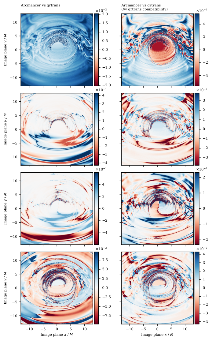
The resulting Stokes intensity maps computed with Arcmancer are shown in Figure 8. In addition, Figure 9 shows the relative differences in the Stokes intensities as computed by Arcmancer versus grtrans. In the left panel of Figure 9, we see that the unpolarized intensity predicted by Arcmancer is consistently higher, and there is a clear difference in the polarized results, especially in the and components.
The reason for this discrepancy was traced to two separate numerical issues. Firstly, grtrans uses values for the gravitational constant and Boltzmann constant that were truncated to three significant figures, while in Arcmancer the CODATA 2014 [79] values are used up to the known experimental precision. Secondly, grtrans uses an approximation for computing the cylindrical Bessel functions used in the relativistic thermal synchrotron radiation model, equations (B4) and (B14) in Dexter [36]. The grtrans code, as well as some other codes, such as [81], use first order approximations for the cylindrical Bessel functions, but at least in this example case the approximations are not always valid throughout.
If the same physical constants and Bessel function approximations are used in Arcmancer, the agreement both in unpolarized and polarized intensities is excellent, as can be seen in the right panel of Figure 9. The unpolarized and polarized total intensities agree with grtrans to a relative level of , and the pixel-by-pixel errors are below percent level on average. There are a small number of high difference outliers located either at regions where the absolute intensity values are very small, or at the strongly lensed rings of emissivity. The former outliers are caused by numerical noise and the latter mainly by spatial sampling noise, since the small scale structure in these rings is not resolved while simultaneously the emission is highly boosted, amplifying the differences. However, it can be seen from the results in Figures 7 and the numerical total fluxes tabulated in Table 1 that these pixels make no significant difference in the observed integrated fluxes.

| Arcmancer | |||
| 1.0083 | 0.98675 | 1.1671 | 1.0054 |
| With grtrans compatibility | |||
| 1.0009 | 1.0029 | 0.99690 | 1.0023 |
| With no polarization | |||
| 1.1264 | 0 | 0 | 0 |
For an interesting test case, we also ran the same test scenario with all polarization effects disabled. That is, we set in and so that only the unpolarized degrees of freedom were propagated. As shown in Table 1, the resulting total flux is higher than in the polarized case. This suggests that creating mock observations of unpolarized flux can be misleading if polarization effects are completely ignored.
VI Applications
The capability of Arcmancer to compute radiation transfer through an emitting and absorbing relativistic fluid (plasma) was showcased in the previous section. In the following, we present further applications of Arcmancer in different scenarios. The focus is on leveraging the capability of Arcmancer to work with all kinds of emitting and absorbing surfaces, both moving and stationary.
VI.1 Effects of thin accretion disk geometry
Arcmancer makes it easy to compute mock observations of emitting surfaces with different user defined geometries. Here this feature is demonstrated through a toy model by computing the changes on the observed spectropolarimetric features caused by varying the opening half-angle of a geometrically thin but optically thick accretion disk around a Kerr black hole.
Often [124, 97, 5, 36, e.g.] a thin disk is modeled in mock observation simulations as an infinitely thin equatorial plane around the black hole. For -disk models [106, 85], this is in many cases a satisfactory approximation. This is because the maximal angle made by the disk photosphere and the symmetry plane is , computed in the Schwarzschild coordinates, where is the black hole accretion rate in units of the Eddington accretion rate . However, for an accretion rate of , this maximal angle is already , which can be expected to have observable consequences. This is since the maximal in the Shakura–Sunyaev solution is found at , where is the black hole mass, which is in the bright inner region of the disk.
Instead of the geometry of the -disk model, which has a photospheric surface profile dependent on the accretion rate, we use a disk defined by a hyperbolic surface in the outgoing Kerr–Schild coordinates,
| (20) |
where is the normalized angular momentum of the black hole, is the half-opening angle of the hyperboloid and sets the inner boundary of the disk, here fixed to the innermost stable circular orbit (ISCO) of the black hole. The choice of this surface is motivated by the intention to investigate only the effects of geometry on the observable properties, while keeping the emission properties of the disk otherwise fixed.
To compute the mock observation, we first set up an image plane with physical dimensions at a distance of (in BL coordinates). From this surface, null geodesics were propagated backwards until they intersected the disk surface or the event horizon. A PolarizationFrame was parallel transported with the geodesic to enable Faraday rotation effects to be captured. Points that hit the disk were given a blackbody spectrum with a temperature matching the Novikov–Thorne disk model [85, 88], using a mass , accretion rate and a dimensionless viscosity parameter . The intensity and the linear polarization of the point were computed based on the electron scattering atmosphere model given in Chandrasekhar [24], using the impact angle between the geodesic and the disk normal, computed in the rest frame of the rotating disk surface. The exact solution requires solving an integral equation. We instead used the Padé approximants
| (21) | ||||
| (22) |
where , for the intensity normalized by the source function (in this example, ), and polarization fraction , respectively. Both approximations are accurate to within over the range . It should be noted that the combination of a blackbody spectrum and a beamed intensity profile is not fully self-consistent, since a genuine blackbody emitter is isotropic. However, the combination serves to illustrate the effects of an anisotropically emitting surface. In addition, the spectral shape for thin accretion disks around stellar mass black holes is in any case well described using a diluted blackbody [34].
To construct the image from these data, instead of running full radiation transfer, the radiation was assumed to propagate in vacuum. This is not a particularly good assumption physically, since the thin disks are expected to have a tenuous, hot coronae [69, 33, e.g.], but it was made so as to not add additional uncertainties and keep the focus on the effects of changing disk geometry. The values of the intensity and polarization were directly transferred to the image plane after scaling the intensity by the redshift factor and rotating the polarization to match the rotation of the parallel transported PolarizationFrame. This computation was repeated for seven values of the disk opening angle from to and three observer inclination angles , and . The results are collected in Figures 10 and 11, which show mock images of the two extreme cases (, ) and the polarization spectra for all the computation runs.

The effect of the disk opening angle is clearly seen in Figure 10, which shows specific intensity maps as seen by an observer at an inclination of for the extreme opening angles of and . The intensity patterns differ significantly, with most of the emission coming from the opposite side of the disk for the disk with the larger opening angle. In addition, the structure of the ring caused by radiation that has traveled around the black hole once is noticeably changed by the increased disk thickness [73, cf.]. Despite the visual differences, Figure 11 shows that the shape of the spectra obtained from the integrated emission is hardly changed at all, and as such the shape of the observed spectrum is not very sensitive to the disk geometry in this example.
Figure 10 also shows a significant difference in polarization patterns, with the large opening angle disk exhibiting a large asymmetry between the upper and lower halves of the mock observation image. This is caused by a purely geometrical effect, wherein the geodesics emanating from the opposite side of the disk from the observer’s point of view are more closely aligned with the local disk surface normal. For the geodesics coming from the observers side of the disk, the situation is the opposite. The polarization fraction of the electron scattering atmosphere model is strongly dependent on the angle of the geodesic with respect to the disk normal, with stronger polarization for lower incidence angles. The graphs of the degree of polarization,
| (23) |
and the polarization angle,
| (24) |
in Figure 11 show that unlike for intensity, the polarization asymmetry does not average out. Indeed, for the largest observer inclination () shown in Figure 11, we see that there is a strong dependency of the degree of net polarization on the disk opening angle . A similar but weaker effect is seen also for the observer inclinations and . Figure 11 also shows the behavior of the net polarization angle . With all observer inclinations, a similar behavior of rotation of the polarization angle at high photon energies is seen. However, for these model parameters, the rotation mainly occurs at the high energy end of the spectrum, where the exponential cutoff makes the effect hard to observe in practice.
The changes in polarization with observation frequency described above, for , are consistent with those of Schnittman & Krolik [104], who studied an infinitely thin disk using a Monte–Carlo approach. However, for a physically more realistic result, the accretion disk corona as well as the radiation returning and reflecting to the disk need to be taken into account, as in Schnittman & Krolik [105]. In addition, here we have shown that the geometry of the optically thick part of the disk cannot be neglected, which is an assumption used in [105]. Combining the effects of the geometry with the effects of the corona and the returning radiation is straightforward using Arcmancer, and will be investigated in a future work.
VI.2 Neutron stars
Another natural application of user-definable surfaces is the imaging of neutron stars. A solid surface is an excellent approximation for the radiating atmosphere of a neutron star, since the atmospheric thickness is on the order of , whereas the radii of the neutron stars are in the range [see e.g. 95, for a review]. Thus terminating geodesics on the top of the atmosphere, and using a separate atmospheric model to provide the (angle-dependent) specific intensity and polarization as initial conditions is an attractive possibility.
The use of a numerical geodesic propagation code such as Arcmancer is further warranted due to the fact that a rotating neutron star is not exactly spherical but oblate, and the space-time near the star cannot be exactly described by the Kerr metric [112, 12, 117]. Both complications are difficult to take into account when using fully analytic approaches, such as in e.g. Pechenick et al. [90], Strohmayer [114], Miller & Lamb [77], Poutanen & Gierliński [96], and Lamb et al. [65], where the neutron star is modeled as a spherical surface in a Schwarzschild space-time. The reason is two-fold: the intersections of geodesics with the oblate surface are much more involved to compute (but not impossible, see Morsink et al. 80, Lo et al. 70, Miller & Lamb 78, Stevens et al. 113), and since the Carter’s constant [20] of the Kerr solution is not available, the geodesics themselves cannot be analytically solved even in quadrature. Another benefit of using a fully covariant approach throughout is that the pitfalls of trying to combine special relativistic and general relativistic effects separately in an ad hoc way (as done in e.g. Lo et al. 70) are avoided. For example, see Nättilä & Pihajoki 83 and Lo et al. 71 for a thorough discussion of an error in the calculation of the observed flux in the ad hoc approach that has gone undetected for years. Finally, incorporating polarization in an analytic geodesic propagator is only possible for Kerr (and Schwarzschild) space-times, but even then it is not trivial [121, 36, see]. However, polarization data for this application is critical, since for small hot spots there is a severe degeneracy in the unpolarized pulse profile between the spot colatitude and the observer inclination [96].
In this section, we use Arcmancer to assess the effects of the oblateness of the neutron star surface and the deviation of the neutron star space-time from the simple Schwarzschild space-time on the radiative transfer calculation. For this purpose, we use the AlGendy–Morsink (AGM) form of the Butterworth–Ipser space-time (AlGendy & Morsink 2, and see also Appendix C.3). The AGM space-time describes the surroundings of a rotating neutron star, taking into account the oblate shape of the star. The space-time is parametrized by the dimensionless rotational parameter , and the compactness parameter , where is the angular velocity of the rotation as seen by a distant observer, and and are the mass and the equatorial radius of the star, respectively. The oblate shape of the star is obtained from equation (C17).
As an example case, we studied a rotating neutron star with a mass , equatorial radius and a rotational frequency of , with . The high value of the spin was chosen to accentuate the effects of oblateness, yielding from equation (C18) a flattening of , where and are the polar and equatorial radii of the star, respectively. However, the high spin value is still within the observed range for neutron stars [55]. Similarly, the mass and the radius are well within the observed and inferred limits [111, 87, 3]. Using Arcmancer, we computed surface maps of flux and polarization characteristics, again assuming that the emission originates from an electron scattering atmosphere, using equations (21) and (22). This is a good approximation for neutron stars where the emission originates from thermonuclear outbursts on the surface [see e.g. 115, and the references therein]. However, we note that the results can be extrapolated on a more qualitative level to shock-heated accretion-powered hot spots as well [6, 74, 121, see e.g.]. Otherwise, the radiation transfer is computed as in Section VI.1.


The computations were repeated three times: for an oblate star using the AGM space-time (hereafter, AGM+Obl), for an oblate star using the Schwarzschild space-time (Sch+Obl) and for a spherical star in the Schwarzschild space-time (Sch+Sph). The results are shown in Figures 12, 13, 14 and 15. Figure 12 shows the behavior of , the specific intensity divided by the source function, and polarization over the star surface, computed using the AGM space-time at observer inclinations of , and . The combination of Doppler boosting and the strong angular dependence of the electron scattering atmosphere yield an intensity that varies significantly over the neutron star surface. The net polarization is high only near the edges, where the impact angle is large. Figure 12 also shows two possible paths of constant colatitude hot spots, assuming that the star is rotating around the vertical axis. From the figure it is then easy to appreciate that a rotating hot spot should exhibit large periodic variation in the observed polarization angle. This variation can be directly seen in Figure 15, which is consistent with the results in Viironen & Poutanen [121].
Figure 13 shows the difference in normalized intensity , degree of polarization and polarization angle when the computation is performed using the AGM metric versus the Schwarzschild metric (i.e., AGM+Obl vs. Sch+Obl). The effects of the rotation become significant only near the star, and consequently the differences stay moderate for the most part, below for the intensity and below for the degree of polarization. There are areas of larger differences, but these are concentrated on the edges of the visible disk of the neutron star, and their total area is small. The differences in the polarization angle are larger, around overall. There are very large differences near the point where the radiation was emitted towards the zenith in the frame of the neutron star surface, but this area corresponds to vanishing polarization, and as such these differences are unobservable.
In contrast, Figure 14 displays the same differences but between computations performed using an oblate star versus a spherical star, both in Schwarzschild space-times (i.e., Sch+Obl vs. Sch+Sph). The spherical star was given a radius equal to the equatorial radius of the oblate star. In this case, the differences in all quantities are much more pronounced. This is not a surprise, since a change in the shape of the star affects the redshift distribution on the surface due to variations in local surface gravity. These differences become even more evident when one looks at Figure 15, which shows two examples of light curves and the time varying degree of polarization and polarization angle for a rotating hot spot. Firstly, the pulse and polarization profiles closely match those obtained by Viironen & Poutanen [121] for the Sch+Sph case, and confirm that the observational degeneracy in unpolarized flux between observer inclination and spot colatitude is lifted by the polarization measurements. However, from the figure it can be seen that the approximation of a spherical star produces results that differ significantly both in intensity and polarization properties from the result obtained using an oblate surface. In addition, there is a small but non-negligible difference between the results obtained using the AGM metric versus a plain Schwarzschild metric. Similar results for the unpolarized flux were obtained already in Psaltis & Özel [98], although for an isotropically emitting atmosphere.
Based on our preliminary study, we can conclude that the error introduced when computing the polarization angle with the Schwarzschild space-time approximation is largest when both the observer inclination and the spot colatitude are small. Likewise, the error in the degree of polarization is largest when the spot is near the equator, i.e. spot colatitude is close to . We conclude that to obtain polarized pulse profiles that are accurate to below the level, it is necessary that the rotation and the geometric shape of the star are both accurately modeled. In practice this means that the analytic results based on the Schwarzschild space-time such as in e.g. Weinberg et al. [127], Viironen & Poutanen [121], Lamb et al. [64], Lo et al. [70] and Miller & Lamb [78] should be used with caution. However, to actually reach level of accuracy, other systematic errors in e.g. modeling the emission from the neutron star and its surrounding environment would also need to be resolved.
VI.3 Binary black holes
To further explore the possibility to use arbitrary metrics and multiple surfaces which may also move, we consider a toy model of an accreting black hole with a secondary black hole companion. To set up the problem, we use an approximative metric, constructed using the outgoing Kerr–Schild form of the Kerr metric, equations (C5) and (C8). In the limit of zero spin, , the metric is
| (25) |
where is the mass of the black hole, ,
| (26) | ||||
| (27) |
and . To this form we add a perturbation representing a distant second black hole moving at a slow coordinate velocity. Taking the spatial position of the second black hole to be a function of the coordinate time, we set
| (28) |
where and are the masses of the primary and secondary black holes, respectively, is the spatial position of the secondary black hole, and .
The metric (28) is not a solution of the vacuum Einstein field equations, for which no exact dynamic binary black hole solution is known.44 4 However, there are a number of known static solutions for multiple black holes. Examples include any number Schwarzschild black holes in a collinear configuration [58], or any number of maximally charged Reissner–Nordström black holes in any configuration [89, 75]. For example, the metric (28) does not contain the gravitational wave component expected from the motion of multiple gravitating bodies. However, in the limit and for all , the perturbation caused by the secondary is small and remains small, and the gravitational wave component is negligible, and in this sense the approximation is reasonable. For black hole binary systems with smaller separations and larger velocities, a discretized metric from a full GR simulation should be used with Arcmancer. More accurate analytical approximations, such as from Mundim et al. [82], can also yield satisfactory accuracy [102], but the approximative analytical metrics are on the other hand algebraically complex.
We set , representing a supermassive black hole (SMBH) and , which falls into the intermediate mass black hole (IMBH) range. Otherwise we set up the system as in Section VI.1, by placing an image plane with physical dimensions at at an observer inclination of . The secondary black hole is set on rectilinear coordinate path , where
| (29) | ||||
| (30) | ||||
Here is the apparent offset of the secondary’s path, is the orthogonal distance from the primary to the image plane, is the minimum distance between the black holes, is the velocity of the secondary and is the angle between the path of the secondary and the image plane -axis. For this particular example, we set , , , and . These initial conditions approximately correspond to an IMBH on a circular orbit around an SMBH, a situation that could possibly follow a merger of a more massive galaxy with a dwarf galaxy [51]. In order to have something to make a mock observation of, the primary black hole was given an infinitely thin Novikov–Thorne accretion disk, with and an accretion rate in units of the Eddington accretion rate. Geodesics were then propagated backwards in time from the image plane starting at different values of the coordinate time, evenly distributed in . For each set of geodesics, mock images, integrated fluxes, and polarization fraction and angle were computed.
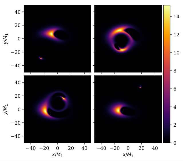
The resulting light curves are shown in Figure 17, with selected resolved frames shown in Figure 16. The main effect of the passing secondary is a strong enhancement by a factor of of the observed flux from the accretion disk of the primary, caused by gravitational lensing. The flux curve has a clearly non-sinusoidal shape, where after the main peak, there is a pronounced shoulder. The double-peaked structure results from the lensing of the two main visible arcs of the primary accretion disk. The difference is that the major peak has a larger contribution from the Doppler boosted side of the primary accretion disk. This asymmetry is also clearly visible in the curves for polarization fraction and angle , see equations (23) and (24). The polarization fraction curve shows a clear two-peaked shape, with a sharp peak followed by a sharp trough. The polarization angle mirrors this behavior, with a maximum rotation of .
The light curves were also computed with a smaller value of observer inclination of , also shown in Figure 17. The results show that the double-peaked structure of the light-curve is more evident towards , whereas the relative amount of polarized flux grows significantly smaller. Both effects are to be expected considering the increased symmetry when . The changes in degree of polarization and the polarization angle are more pronounced as well, but due to the negligible relative amount of polarized flux, these are unlikely to be detectable.
Over longer timescales, the recurrent lensing by the secondary produces a periodic signal, which can be clearly observable over the baseline brightness of the primary accretion disk, as seen from the Figure 17. However, the signal is strongly non-sinusoidal, which may reduce observability in periodicity searches based on periodogram techniques. On the other hand, if a series of accretion disk lensing events was observed, it should be possible to use lensing mock observation simulations to obtain independent constraints on the secondary black hole mass and the orbital parameters.
Finally, we note the interesting fact that the double-peaked light curve is reminiscent of the light curve of the periodic binary blazar OJ 287, which exhibits a long succession of strongly non-sinusoidal double-peaked outbursts every years [109, 118]. Many different physical mechanisms for the outbursts have been proposed, such as tidally enhanced accretion rate [109], accretion disk impacts [68, 93] and changes in the relativistic jet geometry [61, 122]. Accretion disk lensing adds yet another possible outburst mechanism.
VII Conclusions
In this paper, we have presented Arcmancer, a C++/Python library for numerical computation of curves and tensor algebra in arbitrary Riemannian and semi-Riemannian spaces. The library is designed to be easy to extend as well as to incorporate in new or existing applications. Arcmancer offers several novel and useful features. Many of these are built around Arcmancer’s seamless support of multiple simultaneous coordinate charts. For example, Arcmancer offers automatic conversion of coordinates and tensors of arbitrary rank between different charts. This conversion works even in the case where no explicit transformation is provided between two given charts, as long as the graph formed by all the available charts and transformations contains a path connecting the two charts. The coordinate chart support is also used in the library to automatically pick the numerically most appropriate chart to integrate the equations of motion for curves. Arcmancer can also be used for numerical tensor algebra, supporting all usual tensor operations for tensors of arbitrary rank and dimension. In addition, Arcmancer can parallel propagate arbitrary tensors and user-defined quantities along curves. In the four dimensional case, the Arcmancer library contains a suite of tools designed for solving problems of general relativistic radiative transfer using the ray-tracing approach. These include a coordinate-invariant method for generating image planes, easy interface for supplying user-defined fluid and radiation models and a support for geometric objects, which can be used for example to model radiating surfaces or define limits of computational domains. For convenience, the library can also work with either Lorentzian metric signature. All of these features are thoroughly documented in the code itself, in the documention automatically generated from the code and via several example applications provided with the library. In addition, the library website55 5 https://bitbucket.org/popiha/arcmancer provides instructions for installation and getting started.
In this presentation of the Arcmancer library we have included a description of the internal workings of the code, as well as numerous tests of the accuracy of the code. The Arcmancer code was found to fulfill theoretically expected convergence properties. It also produced very similar results as an existing ray-tracing code grtrans, when applied to a demanding mock observation scenario of a hot accretion flow around a Kerr black hole. Notably, the code tests demonstrated the critical importance of choosing the right coordinate system for the chosen problem, and the necessity of being able to change coordinate systems during the numerical evolution of the problem.
The code tests were followed by applications of the code to a variety of astrophysical scenarios, showcasing the flexibility of the Arcmancer code. The first example application was an investigation of the effect of the opening angle of an optically thick but geometrically thin accretion disk to its observable properties. While the unpolarized flux was essentially invariant with respect to the disk opening angle, the degree of polarization and angle of polarization were found to significantly depend on it.
In the next application, Arcmancer was used to study observational properties of hot spots on rotating neutron stars. We compared three different commonly used models. In the AGM+Obl model, the neutron star surface was modeled using a physical oblate shape with an exterior space-time metric that took the oblate shape and rotation into account. This physically accurate model was compared with two more approximate models: Sch+Obl in which the exterior metric was changed to a Schwarzschild metric, and Sch+Sph in which in addition the shape of the neutron star was taken to be spherical. Our results show that the oblate shape of the star makes a large contribution to the shape of both polarized and unpolarized flux curves and must be taken into account. However, we also find that in order to obtain polarized light curves with accuracies better than level, the Schwarzschild metric must be abandoned in favor of more physically motivated alternatives.
Finally, we used Arcmancer to create mock observations of an accreting binary black hole system, consisting of a primary black hole with an accretion disk, together with an orbiting secondary black hole. The application demonstrated how Arcmancer can easily handle a more complex geometry where light rays can be terminated on multiple surfaces (two event horizons and one accretion disk), some of which may move (the secondary event horizon). We found that the lensing caused by the orbiting secondary can produce clearly observable changes in the observed polarized and unpolarized flux from the accretion disk of the primary black hole. However, the changes in polarized flux are strongly dependent on the observer inclination due to the geometry of the simple -disk model we used.
In the future, we expect to use the Arcmancer library to build a comprehensive radiative transfer application for investigating complex accretion flows around compact objects. In addition, the capabilities of the library itself will be extended. Planned features include built-in support for outputs of other GRMHD codes besides HARM, support for easy serialization of the code data structures and more built-in radiation and fluid models. The coordinate chart system will also be enhanced with support for defining domains for the charts, and improving the numerical behavior of chart-dependent operations such as curve interpolation.
Ray-tracing is expected to become even more important in the future, driven by the increase in observational capabilities, especially with respect to polarized light, together with the ongoing prodigious increase in computational resources. We are confident that Arcmancer will prove to be a highly useful and adaptable tool in this upcoming era.
Appendix A Differential geometry and General Relativity
The Arcmancer library has capabilities beyond ray-tracing and radiative transfer in four-dimensional Lorentzian space-times. The library offers a variety of tools for computational differential geometry in Riemannian or semi-Riemannian manifolds of arbitrary dimension, within the constraints of available memory and computing power. In the following, we give a short, self-contained review of the concepts of differential geometry that are implemented and used in the Arcmancer library. For practical reasons the exposition is kept brief and mathematical details are omitted where possible. The discussion is styled after a number of texts, namely Lee [67], O’Neill [86], Lee [66] and Choquet-Bruhat et al. [27], in which the interested reader can find the omitted details.
A.1 Manifolds and coordinate charts
The basic building block of differential geometry is the manifold , which can be intuitively understood as a space which locally ‘looks like’ , the -dimensional Euclidean space. More concretely, each manifold comes with an atlas of charts (coordinate systems) , defined on open sets of . Using a chart , an abstract point is transformed into its coordinate representation , where is the projection to the ’th coordinate. We say that the dimension of is , and use the shorthand . A change in coordinates then corresponds to the transition map , which changes a tuple of coordinates to another tuple of coordinates, describing the same point. Arcmancer requires the manifold to be differentiable, meaning that the maps are differentiable. However, in the following we assume smooth (infinitely differentiable) manifolds.
A.2 Tensors
The tangent space of at point , written , is the space of all vectors tangent to at . If , then is an -dimensional real vector space. The dual space of , written and called the cotangent space of at , is the space of all linear maps . These linear maps are called one-forms. For each chart , at point we can define the vectors , called coordinate vectors. The vector points towards the direction where the ’th coordinate increases at . The complete set of coordinate vectors, , forms a basis for , called the coordinate basis. Any vector can be written in terms of its components in this special basis, as , where now are the components of in the chart and the Einstein summation convention has been assumed. Likewise, there exists a set of one-forms, called the coordinate one-forms, which form a basis for , and make it possible to write any one-form in terms of its components as . The coordinate vectors and one-forms obey , where is the Kronecker delta symbol. Together, the coordinate vectors and one-forms are called the coordinate frame. The tangent and cotangent spaces can naturally have other bases than coordinate bases as well (see A.6), but the coordinate basis is the default basis used in Arcmancer.
A rank tensor can then be defined as a multilinear map . In general, the factors and may be in any order, and the ordering is important, but for convenience, we will use the ordering given above. A rank corresponds to scalar quantity, and rank tensors are equivalent to vectors, and rank tensors to one-forms. The components of a tensor at in the coordinate basis can be directly found from
| (A1) |
Using the components, a tensor can be locally defined as an expansion
| (A2) |
If instead of the chart we wish to use another (overlapping) chart to represent the tensor , the components of a tensor must be transformed accordingly. The new components turn out to be
| (A3) |
where are the components of the Jacobian of the function at point , and similarly for the inverse of the Jacobian .
The definitions above generalize to vector, one-form and tensor fields, which can be understood as functions which, for each point of , pick a specific vector, one-form or tensor, respectively. In physics-oriented GR literature, all tensorial quantities are usually tensor fields. In addition, a convention called the abstract index notation [91] is often used. In this convention, for example, a rank tensor field can be written as . The number and ordering of the upper and lower indexes is taken only to signify the number and ordering of the factors and in the definition (A2) of the tensor. This approach makes it possible to write all coordinate invariant tensor operations tersely, without specifying any underlying basis. In this paper, we use the abstract index notation wherever possible.
A.3 Metric
A manifold may have a special rank tensor field called the metric, usually written . The metric defines the inner product of vectors , and consequently a norm on each . Intuitively, the metric defines the distance between nearby points and as the norm of the tangent vector approximated by . In physics, the components of the metric are often written in the form of a line element , essentially an expansion in terms of coordinate basis tensors, as . The signature of the metric is the pair of the number of positive and negative eigenvalues of the matrix of components of (in any basis), respectively, assuming . If , the metric and the manifold are said to be Riemannian. For signatures or the metric and the manifold are said to be Lorentzian. In particular, General Relativity is defined in terms of a four-dimensional Lorentzian manifold. In this paper, Lorentzian metrics are always assumed to be of type , and in particular for GR this implies the metric convention.
A choice of metric also defines a unique metric-compatible zero-torsion connection , often called the Levi–Civita connection. A connection in general can be roughly said to characterize which vectors of the tangent spaces of two nearby points are to be considered equal, or alternatively, to yield a vector field describing the rate of change of the vector field in the direction of the vector field , called the (natural) covariant derivative of with respect to . Written in terms of the coordinate vector fields, the connection is , where are the Christoffel symbols (of the second kind). This work only uses the Levi–Civita connection, the zero-torsion property of which can be written as , and the metric compatibility as . In terms of the metric, the Christoffel symbols read
| (A4) |
The covariant derivative can be generalized for any tensor field . Using the Christoffel symbols, the covariant derivative of with respect to can be written in component form as
| (A5) |
In the abstract index notation the covariant derivative is written simply as . The term covariant derivative of , without additional qualifiers, is often used to refer only to the vector field independent part . If , we say that is parallel (transported) along the vector field . This concept can be extended to the case where is a tangent vector field of a curve , see below.
For semi-Riemannian spaces, the metric also divides vectors at a point into three categories. A vector is said to be timelike if the inner product is positive, null if it is zero, and spacelike otherwise. The same classification can be extended to vector fields if the sign of the inner product is the same everywhere on .
A.4 Geodesics and other curves
For ray-tracing mock observations, the notion of curves and especially geodesics on a manifolds is essential. A curve can be thought of as a map . The curve defines a vector field through along the curve. This vector field can be understood as the velocity vector field of the curve. The curve itself is a solution of
| (A6) |
If in particular , the tangent vector of the curve is parallel transported along the curve, and we say that the curve is a geodesic. Equation (A6) can also be written as
| (A7) |
where the vector field is analogous to a force, which causes the curve to deviate from a straight path along the manifold. For geodesics, , corresponding to the notion of geodesics as the straightest possible paths. Written in terms of components in a specific chart, equation (A7) reads
| (A8) |
In this form the equation can be solved numerically, as long as the solution stays within the domain of the chart.
Generic tensorial quantities can also be parallel transported along the curve. For a rank tensor field the equation of parallel transport is
| (A9) |
which in component form can be found from equation (A5) with the substitution . Equation (A9) can likewise be directly solved numerically.
Finally, curves for which the tangent vector field is always timelike, spacelike or null, are called timelike, spacelike or null, respectively. This characterization is important for geodesics, for which the tangent vector field can never change their timelike, spacelike or null character. As such, geodesics always fall in one of these categories.
A.5 Level hypersurfaces
Manifolds may contain many kinds of submanifolds. A particularly useful class of submanifolds are those defined by level sets of functions, called level hypersurfaces. If is a smooth map, then the sets are submanifolds of for each in the codomain of if for all . We can subsume the constant in the definition of the function and take , which is always assumed in the Arcmancer code. Furthermore, with a slight abuse of notation, we use the function defining the hypersurface to refer to the hypersurface itself.
A level hypersurface divides the manifold into two disconnected subsets corresponding to regions where the value of is negative or positive. In some cases, these may be conveniently taken to be the ‘outside’ and the ‘inside’ of a region bounded by the level hypersurface.
A.6 Local frames
Tensor fields can also be expressed in terms of other bases than the coordinate basis. A local frame defined in an open set consists of vector fields that form a basis for at each . For each local frame, there is a corresponding local coframe of one-form fields for which . The components of a rank tensor in terms of these bases can then be defined through (see equation (A1))
| (A10) |
The transformation from the components of a tensor in a coordinate frame to components in terms of a local frame can be found by first writing the local (co)frame in terms of the coordinate frame as and . Using the multilinearity of an arbitrary -tensor in equation (A10) then yields
| (A11) |
where are the components of the tensor in the coordinate frame. From a computational perspective, it is useful to note that the set of numbers can be interpreted as a matrix, for which the corresponding set forms an inverse matrix. The equation (A11) is seen to resemble the equation (A3), with these matrices taking the place of the Jacobians.
Orthonormal local frames define a set of convenient projections of into orthogonal complements at each point . A collection of non-null basis vectors , defines a projection onto the subspace of spanned by through
| (A12) |
Similarly, a projection onto the orthogonal complement of this subspace is defined via
| (A13) |
For Lorentzian spaces, direct projections with respect to a null vector do not work. However, given a unit timelike vector , a projection onto the space orthogonal to both and can be given through
| (A14) |
where and . In four dimensions, the operator is a projection onto a two-dimensional surface on which the observed components of polarization are defined. In this context, is known as the screen projection operator [44].
A.6.1 Lorentz frames and observers
In the case of a four-dimensional Lorentzian manifold, an orthonormal local frame is often called a (local) Lorentz frame or a tetrad. The tetrad can in general consist of any permissible combination of null, spacelike and timelike vector fields. However, in this work we use the term Lorentz frame to mean a mutually orthonormal combination of one timelike vector and three spacelike vectors , and , defined at a point. Since parallel transport preserves inner products, a parallel transported Lorentz frame is still a valid Lorentz frame.
Observers in GR are characterized by a timelike curve , a world line. An observer’s rest frame can then be defined as a Lorentz frame for which the timelike basis vector is given by the observer’s four-velocity, or , and the spatial triad defines the observer’s choice of spatial coordinate system. The values of physical quantities as measured by the observer are obtained by expressing them in the observer’s rest frame basis.
For example, an important feature of GR is that angles between vectors at a point is observer dependent. The angle between vectors and as measured by an observer with a four-velocity is then
| (A15) |
where and .
Appendix B Radiative transfer
B.1 Geometric optics
Briefly, a propagating monochromatic radiation front can be modeled as a congruence of curves, each perpendicular to the surface of constant phase. This is possible in the limit where, the wavelength of the radiation is much smaller than the scale of variations in the radiation front (curvature, amplitude, polarization) and much smaller than the local ‘radius of curvature of the space’ , where is the Riemann curvature tensor.
Furthermore, if the contribution of matter is insignificant, i.e. , the result is that the propagation of radiation can be modeled by solving an equation of radiative transfer along null geodesics. If the integrated contribution of the intervening matter is non-negligible, the radiation front normals will not be geodesics in general, and there will be a matter-dependent forcing term in equation (A7) (see e.g. Broderick & Blandford 13 and Broderick & Blandford 14).
B.2 Equation of radiative transfer
The classical equation of radiative transfer in Cartesian coordinates is [76]
| (B1) |
where is the total emission coefficient (emissivity) and the total absorption coefficient. The equation (B1) describes the change in specific intensity at frequency in the direction at a point and time . Often in astrophysical cases, the one-dimensional time-independent case suffices, in which case the equation (B1) reduces to a more commonly seen form
| (B2) |
where is the distance along a radiation front normal. The equations (B1) and (B2) do not take into account interference, quantum effects or, most importantly, polarization.
Polarization can be included by making the specific intensity vector valued, introducing the Stokes intensities . Similarly, is replaced by the vector
| (B3) |
of Stokes emissivities and by the response (or Müller) matrix
| (B4) |
where the -coefficients represent absorption effects, and the -coefficients relate to Faraday conversion and rotation. It should be noted that different conventions for exist, varying by the sign of . The one-dimensional polarized equation of radiative transfer is then
| (B5) |
The general relativistic generalization of equation (B5) is [44, e.g.]
| (B6) |
where is the affine parameter along the curve representing the propagating radiation front, is the (complex-valued) polarization tensor, is the emissivity tensor and is the response tensor.
Directly solving equation (B6) requires integrating the 16 real independent components of . This number can be reduced to four by parallel transporting a polarization frame along the geodesic. The frame consists of two orthogonal spacelike vectors also orthogonal to the geodesic and the observer four-velocity. Expressing all quantities in this frame using the screen projection operator (A14), the equation (B6) can be written as
| (B7) |
where , , and is a constant related to the parametrization of the curve. An observer with a four-velocity at one end of the curve, where the tangent is , has for an observed frequency .
Appendix C Built-in manifold and chart support
Arcmancer contains a number of predefined metric spaces and space-times together with commonly used coordinate charts for convenience. The number of implemented spaces and charts is expected to grow, but the selection at the time of writing is given in the following. We list all the charts and the representations of the metric, either as a line element or in matrix form, in these charts for each implemented space. All Lorentzian space-times are shown with the metric convention.
C.1 Riemannian manifolds
C.1.1 Two-sphere
Spherical coordinates
Arcmancer uses two copies of the spherical chart to cover the entire two-sphere. The metric, in either copy, is given by the usual
| (C1) |
C.2 Semi-Riemannian manifolds
C.2.1 Minkowski space-time
Cartesian coordinates
The Cartesian Minkowski coordinates are often in the literature denoted by , and we use the same convention. The line element is diagonal, given by
| (C2) |
Spherical coordinates
| (C3) |
C.2.2 Kerr space-time
The Kerr space-time [63] is an important solution to the Einstein field equations, representing a rotating black hole exactly, and other rotating fluid bodies of finite size asymptotically. The Kerr space-time is parametrized by the mass and the angular momentum . Usually is given through the normalized spin parameter , in which case or the dimensionless spin parameter , so that . The solution reduces to the Schwarzschild space-time when and further to the flat Minkowski space-time when .
Boyer–Lindquist coordinates
Perhaps the clearest representation of the Kerr metric in the Boyer–Lindquist (BL) coordinates is through the matrix form
| (C4) |
where and . The BL form of the metric is singular when or . The former condition corresponds to , which give the locations of the inner and outer event horizons, where the curvature is not singular. The condition implies and , and corresponds to the curvature singularity.
Cartesian Kerr–Schild coordinates
The Cartesian Kerr–Schild (KS) coordinates come in two flavors, ingoing and outgoing, adapted to null geodesics that move radially inwards or outwards, respectively. As such, they are a generalization of the ingoing and outgoing Eddington–Finkelstein coordinates for a Schwarzschild black hole. Of the two variants, only the ingoing form is typically seen in the literature. The metric in the ingoing KS coordinates is most easily written as a sum
| (C5) |
where is the Cartesian Minkowski metric,
| (C6) | ||||
| (C7) |
and is defined implicitly through . The vector is null with respect to both and . The metric in the outgoing coordinates is similarly given by a sum as in equation (C5), but with
| (C8) |
When numerically computing geodesics near a Kerr black hole, it is crucial that the right form of the KS coordinates is chosen. If the geodesic approaches the hole, the ingoing chart should be used, and for a geodesic going away from the hole, the outgoing chart should be used. Failure to do so has significant computational penalties, as can be seen in Section V.1.2. Note that this implies that for a geodesic coming in towards a Kerr black hole, passing by it, and then leaving, both ingoing and outgoing charts should be used with a change of coordinates near the closest approach.
C.3 AlGendy–Morsink (AGM) space-time
AGM coordinates
The AGM space-time and coordinates [2] actually refer to a specific choice of a Butterworth–Ipser (BI) space-time, with the accompanying coordinate chart [18]. The BI space-time is a general representation of the space-time outside an axisymmetric rotating fluid body. The AGM space-time is a special case representing the space-time around a physically realistic oblate rotating neutron star. The AGM representation is accurate up to second order in the dimensionless rotation parameter , where is the rotational angular velocity of the star as seen by a distant observer, is the equatorial radius of the star and is the mass of the star. In the BI coordinates, the generic axisymmetric metric reads
| (C9) |
where , , and are so-called metric functions or potentials. The AGM metric is defined by using
| (C10) | ||||
| (C11) | ||||
| (C12) | ||||
| (C13) |
where is the second order Legendre polynomial. The constants and are the dimensionless moments of energy density and pressure, respectively, and is the dimensionless angular momentum. AlGendy & Morsink [2] found these constants to be well described across various neutron star parameters and equations of state by the approximate relations
| (C14) | ||||
| (C15) | ||||
| (C16) |
where is called the compactness (parameter). Along with the metric potentials, AlGendy & Morsink [2] also derived an equation for the shape of the surface of a rotating neutron star, used in Section VI.2,
| (C17) |
From this, the flattening, also called oblateness, of the star is given by
| (C18) |
It should be noted that the quantities and are not defined in terms , but instead in terms of a radial coordinate .
C.4 Hartle–Thorne space-time
The Hartle–Thorne (HT) space-time [53] describes the space-time around a rotating oblate star. The original derivation was based on a perturbation of the non-rotating Schwarzschild space-time. In Arcmancer, we use instead a version based on a perturbation of the rotating Kerr space-time, given in Glampedakis & Babak [48].
Glampedakis–Babak (GB) coordinates
The GB coordinates are based on the Boyer–Lindquist coordinates of the Kerr space-time. In these coordinates, in a parametrization used by Bauböck et al. [9], the metric is given by
| (C19) |
where is the Kerr metric in the BL coordinates (see eq. (C4)), and
| (C20) | ||||||
| (C21) |
Here is the mass of the star, is the dimensionless angular momentum and parametrizes the mass quadrupole moment , so that corresponds to the quadrupole moment of the Kerr space-time. The functions are given in Glampedakis & Babak [48].
References
- [1] Ahnert, K., & Mulansky, M. 2011, AIP Conference Proceedings, 1389, 1586
- [2] AlGendy, M., & Morsink, S. M. 2014, ApJ, 791, 78
- [3] Alsing, J., Silva, H. O., & Berti, E. 2017, ArXiv e-prints, arXiv:1709.07889
- [4] Atamurotov, F., Ghosh, S. G., & Ahmedov, B. 2016, European Physical Journal C, 76, 273
- [5] Bambi, C. 2012, ApJ, 761, 174
- [6] Basko, M. M., & Sunyaev, R. A. 1976, MNRAS, 175, 395
- [7] Bauböck, M., Özel, F., Psaltis, D., & Morsink, S. M. 2015a, ApJ, 799, 22
- [8] Bauböck, M., Psaltis, D., & Özel, F. 2015b, ApJ, 811, 144
- [9] Bauböck, M., Psaltis, D., Özel, F., & Johannsen, T. 2012, ApJ, 753, 175
- [10] Beloborodov, A. M. 2002, ApJ, 566, L85
- [11] Bower, G. C., Markoff, S., Dexter, J., et al. 2015, ApJ, 802, 69
- [12] Bradley, M., & Fodor, G. 2009, Phys. Rev. D, 79, 044018
- [13] Broderick, A., & Blandford, R. 2003, MNRAS, 342, 1280
- [14] Broderick, A., & Blandford, R. 2004, MNRAS, 349, 994
- [15] Broderick, A. E. 2004, PhD thesis, California Institute of Technology, California, USA
- [16] Broderick, A. E., Fish, V. L., Johnson, M. D., et al. 2016, ApJ, 820, 137
- [17] Bromley, B. C., Melia, F., & Liu, S. 2001, ApJ, 555, L83
- [18] Butterworth, E. M., & Ipser, J. R. 1976, ApJ, 204, 200
- [19] Cadeau, C., Morsink, S. M., Leahy, D., & Campbell, S. S. 2007, ApJ, 654, 458
- [20] Carter, B. 1968, Physical Review, 174, 1559
- [21] Chael, A. A., Johnson, M. D., Narayan, R., et al. 2016, ApJ, 829, 11
- [22] Chan, C.-k., Medeiros, L., Ozel, F., & Psaltis, D. 2017, ArXiv e-prints, arXiv:1706.07062
- [23] Chan, C.-k., Psaltis, D., & Özel, F. 2013, ApJ, 777, 13
- [24] Chandrasekhar, S. 1960, Radiative transfer (New York: Dover)
- [25] Chen, B., Kantowski, R., Dai, X., Baron, E., & Maddumage, P. 2015, ApJS, 218, 4
- [26] Chen, K., Halpern, J. P., & Filippenko, A. V. 1989, ApJ, 339, 742
- [27] Choquet-Bruhat, Y., DeWitt-Morette, C., & Dillard-Bleick, M. 1982, Analysis, Manifolds, and Physics, Analysis, Manifolds, and Physics No. Part 1 (Amsterdam, Netherlands: North-Holland Publishing Company)
- [28] Connors, P. A., & Stark, R. F. 1977, Nature, 269, 128
- [29] Connors, P. A., Stark, R. F., & Piran, T. 1980, ApJ, 235, 224
- [30] Cunningham, C. 1976, ApJ, 208, 534
- [31] Cunningham, C. T. 1975, ApJ, 202, 788
- [32] Cunningham, C. T., & Bardeen, J. M. 1972, ApJ, 173, L137
- [33] Czerny, B., & Elvis, M. 1987, ApJ, 321, 305
- [34] Davis, S. W., Blaes, O. M., Hubeny, I., & Turner, N. J. 2005, ApJ, 621, 372
- [35] De Falco, V., Falanga, M., & Stella, L. 2016, A&A, 595, A38
- [36] Dexter, J. 2016, ArXiv e-prints, arXiv:1602.03184
- [37] Dexter, J., & Agol, E. 2009, ApJ, 696, 1616
- [38] Doeleman, S., Agol, E., Backer, D., et al. 2009, in Astronomy, Vol. 2010, astro2010: The Astronomy and Astrophysics Decadal Survey
- [39] Dormand, J., & Prince, P. 1980, Journal of Computational and Applied Mathematics, 6, 19
- [40] Ebisawa, K., Mitsuda, K., & Hanawa, T. 1991, ApJ, 367, 213
- [41] Eisenhauer, F., Perrin, G., Brandner, W., et al. 2008, in Proc. SPIE, Vol. 7013, Optical and Infrared Interferometry, 70132A
- [42] Falcke, H., Melia, F., & Agol, E. 2000, ApJ, 528, L13
- [43] Fukue, J., & Yokoyama, T. 1988, PASJ, 40, 15
- [44] Gammie, C. F., & Leung, P. K. 2012, ApJ, 752, 123
- [45] Gammie, C. F., McKinney, J. C., & Tóth, G. 2003, ApJ, 589, 444
- [46] García, F., Ranea-Sandoval, I. F., & Johannsen, T. 2016, A&A, 587, A141
- [47] Gendreau, K. C., Arzoumanian, Z., & Okajima, T. 2012, in Proc. SPIE, Vol. 8443, Space Telescopes and Instrumentation 2012: Ultraviolet to Gamma Ray, 844313
- [48] Glampedakis, K., & Babak, S. 2006, Classical and Quantum Gravity, 23, 4167
- [49] Gold, R., McKinney, J. C., Johnson, M. D., & Doeleman, S. S. 2017, ApJ, 837, 180
- [50] González Caniulef, D., Zane, S., Taverna, R., Turolla, R., & Wu, K. 2016, MNRAS, 459, 3585
- [51] Graham, A. W., & Scott, N. 2013, ApJ, 764, 151
- [52] Hairer, E., Nørsett, S., & Wanner, G. 2008, Solving Ordinary Differential Equations I: Nonstiff Problems, Springer Series in Computational Mathematics (Heidelberg, Germany: Springer-Verlag)
- [53] Hartle, J. B., & Thorne, K. S. 1968, ApJ, 153, 807
- [54] Henon, M. 1982, Physica D Nonlinear Phenomena, 5, 412
- [55] Hessels, J. W. T., Ransom, S. M., Stairs, I. H., et al. 2006, Science, 311, 1901
- [56] Hunter, J. D. 2007, Computing In Science & Engineering, 9, 90
- [57] Ishihara, H., Takahashi, M., & Tomimatsu, A. 1988, Phys. Rev. D, 38, 472
- [58] Israel, W., & Khan, K. A. 1964, Il Nuovo Cimento, 33, 331
- [59] Jaroszynski, M., Wambsganss, J., & Paczynski, B. 1992, ApJ, 396, L65
- [60] Karas, V., Vokrouhlicky, D., & Polnarev, A. G. 1992, MNRAS, 259, 569
- [61] Katz, J. I. 1997, ApJ, 478, 527
- [62] Kelly, B. J., Baker, J. G., Etienne, Z. B., Giacomazzo, B., & Schnittman, J. 2017, Phys. Rev. D, 96, 123003
- [63] Kerr, R. P. 1963, Physical Review Letters, 11, 237
- [64] Lamb, F. K., Boutloukos, S., Van Wassenhove, S., et al. 2009a, ApJ, 706, 417
- [65] Lamb, F. K., Boutloukos, S., Van Wassenhove, S., et al. 2009b, ApJ, 705, L36
- [66] Lee, J. 2006, Riemannian Manifolds: An Introduction to Curvature, Graduate Texts in Mathematics (New York, NY, USA: Springer)
- [67] Lee, J. 2013, Introduction to Smooth Manifolds, Graduate Texts in Mathematics (New York, NY, USA: Springer)
- [68] Lehto, H. J., & Valtonen, M. J. 1996, ApJ, 460, 207
- [69] Liang, E. P. T., & Price, R. H. 1977, ApJ, 218, 247
- [70] Lo, K. H., Miller, M. C., Bhattacharyya, S., & Lamb, F. K. 2013, ApJ, 776, 19
- [71] Lo, K. H., Miller, M. C., Bhattacharyya, S., & Lamb, F. K. 2018, ArXiv e-prints, arXiv:1801.08031
- [72] Ludlam, R. M., Miller, J. M., Cackett, E. M., et al. 2016, ApJ, 824, 37
- [73] Luminet, J.-P. 1979, A&A, 75, 228
- [74] Lyubarskii, Y. E., & Syunyaev, R. A. 1982, Soviet Astronomy Letters, 8, 330
- [75] Majumdar, S. D. 1947, Phys. Rev., 72, 390
- [76] Mihalas, D., & Mihalas, B. W. 1984, Foundations of radiation hydrodynamics (Oxford University Press, New York)
- [77] Miller, M. C., & Lamb, F. K. 1998, ApJ, 499, L37
- [78] Miller, M. C., & Lamb, F. K. 2015, ApJ, 808, 31
- [79] Mohr, P. J., Newell, D. B., & Taylor, B. N. 2016, Reviews of Modern Physics, 88, 035009
- [80] Morsink, S. M., Leahy, D. A., Cadeau, C., & Braga, J. 2007, ApJ, 663, 1244
- [81] Mościbrodzka, M., & Gammie, C. F. 2018, MNRAS, 475, 43
- [82] Mundim, B. C., Nakano, H., Yunes, N., et al. 2014, Phys. Rev. D, 89, 084008
- [83] Nättilä, J., & Pihajoki, P. 2017, ArXiv e-prints, arXiv:1709.07292
- [84] Noble, S. C., Gammie, C. F., McKinney, J. C., & Del Zanna, L. 2006, ApJ, 641, 626
- [85] Novikov, I. D., & Thorne, K. S. 1973, in Black Holes (Les Astres Occlus), ed. C. Dewitt & B. S. Dewitt, 343–450
- [86] O’Neill, B. 1983, Semi-Riemannian Geometry With Applications to Relativity, Pure and Applied Mathematics (Sand Diego, CA, USA: Academic Press)
- [87] Özel, F., & Freire, P. 2016, ARA&A, 54, 401
- [88] Page, D. N., & Thorne, K. S. 1974, ApJ, 191, 499
- [89] Papapetrou, A. 1945, Proceedings of the Royal Irish Academy. Section A: Mathematical and Physical Sciences, 51, 191
- [90] Pechenick, K. R., Ftaclas, C., & Cohen, J. M. 1983, ApJ, 274, 846
- [91] Penrose, R., & Rindler, W. 1987, Spinors and Space-Time: Volume 1, Two-Spinor Calculus and Relativistic Fields, Cambridge Monographs on Mathematical Physics (Cambridge, UK: Cambridge University Press)
- [92] Pihajoki, P. 2015, Celestial Mechanics and Dynamical Astronomy, 121, 211
- [93] Pihajoki, P. 2016, MNRAS, 457, 1145
- [94] Porth, O., Olivares, H., Mizuno, Y., et al. 2017, Computational Astrophysics and Cosmology, 4, 1
- [95] Potekhin, A. Y. 2014, Physics Uspekhi, 57, 735
- [96] Poutanen, J., & Gierliński, M. 2003, MNRAS, 343, 1301
- [97] Psaltis, D., & Johannsen, T. 2012, ApJ, 745, 1
- [98] Psaltis, D., & Özel, F. 2014, ApJ, 792, 87
- [99] Rauch, K. P., & Blandford, R. D. 1991, ApJ, 381, L39
- [100] Rauch, K. P., & Blandford, R. D. 1994, ApJ, 421, 46
- [101] Riffert, H., & Meszaros, P. 1988, ApJ, 325, 207
- [102] Sadiq, J., Zlochower, Y., & Nakano, H. 2018, ArXiv e-prints, arXiv:1802.02990
- [103] Savitzky, A., & Golay, M. J. E. 1964, Analytical Chemistry, 36, 1627
- [104] Schnittman, J. D., & Krolik, J. H. 2009, ApJ, 701, 1175
- [105] Schnittman, J. D., & Krolik, J. H. 2010, ApJ, 712, 908
- [106] Shakura, N. I., & Sunyaev, R. A. 1973, A&A, 24, 337
- [107] Shcherbakov, R. V., & Huang, L. 2011, MNRAS, 410, 1052
- [108] Shcherbakov, R. V., & McKinney, J. C. 2013, ApJ, 774, L22
- [109] Sillanpaa, A., Haarala, S., Valtonen, M. J., Sundelius, B., & Byrd, G. G. 1988, ApJ, 325, 628
- [110] Stark, R. F., & Connors, P. A. 1977, Nature, 266, 429
- [111] Steiner, A. W., Lattimer, J. M., & Brown, E. F. 2016, European Physical Journal A, 52, 18
- [112] Stergioulas, N. 2003, Living Reviews in Relativity, 6, 3
- [113] Stevens, A. L., Fiege, J. D., Leahy, D. A., & Morsink, S. M. 2016, ApJ, 833, 244
- [114] Strohmayer, T. E. 1992, ApJ, 388, 138
- [115] Suleimanov, V., Poutanen, J., & Werner, K. 2011, A&A, 527, A139
- [116] Treu, T. 2010, ARA&A, 48, 87
- [117] Urbanec, M., Miller, J. C., & Stuchlík, Z. 2013, MNRAS, 433, 1903
- [118] Valtonen, M. J., Lehto, H. J., Nilsson, K., et al. 2008, Nature, 452, 851
- [119] van der Walt, S., Colbert, S. C., & Varoquaux, G. 2011, Computing in Science Engineering, 13, 22
- [120] Viergutz, S. U. 1993, A&A, 272, 355
- [121] Viironen, K., & Poutanen, J. 2004, A&A, 426, 985
- [122] Villata, M., Raiteri, C. M., Sillanpaa, A., & Takalo, L. O. 1998, MNRAS, 293, L13
- [123] Vincent, F. H., Gourgoulhon, E., Herdeiro, C., & Radu, E. 2016, Phys. Rev. D, 94, 084045
- [124] Vincent, F. H., Paumard, T., Gourgoulhon, E., & Perrin, G. 2011, Classical and Quantum Gravity, 28, 225011
- [125] Vincent, F. H., Bejger, M., Rozanska, A., et al. 2017, ArXiv e-prints, arXiv:1711.02414
- [126] Weinberg, D. H., Mortonson, M. J., Eisenstein, D. J., et al. 2013, Phys. Rep., 530, 87
- [127] Weinberg, N., Miller, M. C., & Lamb, D. Q. 2001, ApJ, 546, 1098
- [128] Zhang, S. N., Feroci, M., Santangelo, A., et al. 2016, in Proc. SPIE, Vol. 9905, Space Telescopes and Instrumentation 2016: Ultraviolet to Gamma Ray, 99051Q