Differentially passive circuits
that switch and oscillate
Abstract
The concept of passivity is central to analyze circuits as interconnections of passive components. We illustrate that when used differentially, the same concept leads to an interconnection theory for electrical circuits that switch and oscillate as interconnections of passive components with operational amplifiers (op-amps). The approach builds on recent results on dominance and -passivity aimed at generalizing dissipativity theory to the analysis of non-equilibrium nonlinear systems. Our paper shows how those results apply to basic and well-known nonlinear circuit architectures. They illustrate the potential of dissipativity theory to design and analyze switching and oscillating circuits quantitatively, very much like their linear counterparts.
keywords
switches, oscillators, differential passivity1 Introduction
The concept of passivity originates in circuit theory. It characterizes circuit elements that can possibly store and dissipate the energy provided by the environment, but not the other way around. Passivity is inherently an interconnection concept: passive interconnections of passive components model passive circuits. Dissipativity theory, the system theoretic generalization of passivity theory, has become a cornerstone of system theory. It provides an interconnection theory to design and analyze stable dynamical systems. Such systems dissipate the energy stored internally and provided externally. In short, dissipativity theory is an interconnection theory for Lyapunov stability analysis. In recent years, many researchers have pointed to the relevance of studying stability incrementally or differentially when addressing questions that go beyond the stability analysis of isolated equilibria. Differential stability concepts include contraction theory (Lohmiller and Slotine, 1998), convergence theory (Pavlov et al., 2005), or differential Lyapunov theory (Forni and Sepulchre, 2014). They have proven relevant in a number of areas, most prominently in questions pertaining to nonlinear observers (Aghannan and Rouchon, 2003), oscillator synchronization (Stan and Sepulchre, 2007), or regulation theory (Jouffroy and Fossen, 2010). Differential dissipativity is to differential stability what dissipativity is to Lyapunov stability. It was introduced in the recent papers (Forni et al., 2013; Forni and Sepulchre, 2013; van Der Schaft, 2013). The present paper aims at illustrating the potential of differential passivity as an interconnection theory of circuits that can switch an oscillate. In contrast with classical dissipativity theory, such a theory must cope with the stability analysis of dynamical systems that posses multiple equilibria or limit cycles. It is based on the concept of -dominance and -passivity recently introduced in Forni and Sepulchre (2017a); Forni and Sepulchre (2017b). Intuitively, the attractors of a -dominant system are the attractors of a -dimensional system: a unique equilibrium for , but possibly multiple equilibria for , and limit cycles for . We interpret classical differential dissipativity theory as an interconnection theory for -dominance, that is, differential stability. The extension to and is motivated by the analysis of multistability or limit cycles in interconnected systems. Nonlinear circuit theory provides a realm of switching and oscillatory behaviors designed from the simple elements of linear circuit theory interconnected with operational amplifiers (op-amp) (Clayton and Winder, 2003). Our aim in the present paper is to illustrate that those building blocks are the natural building blocks of -passive circuits. System theoretic tools have lacked so far for the quantitative analysis and design of such circuits. Their analysis normally rests on simplifying assumptions, time-scale separation arguments leading to asymptotic analysis, or reductions to two-dimensional phase portraits. In contrast, we are aiming at quantitative and computationally tractable certificates such as those used in the theory of linear time-invariant systems. Such tools have made the success of robustness and performance analysis of linear time-invariant systems. A pillar of passivity theory is the passivity theorem, which states that the negative feedback interconnection of two passive systems is passive. It is also well-known that switches and oscillatory circuits require both positive and negative feedback interconnections of op-amps with passive elements. We stress in the present paper that such interconnections fall in the category of the -passivity theorem, which states that the negative feedback interconnection of a -passive with a -passive circuit is passive.
The differential analysis in this paper assumes smooth systems. A companion paper shows that an analog framework exists for non-smooth systems. To account for the lack of differentiability, differential concepts have then to be replaced by incremental concepts. Many of the nonlinear circuits discussed in the present paper have a non-smooth analog that falls in the category of linear complementarity systems studied in Miranda-Villatoro et al. (2018). The rest of the paper is organized as follows. Section 2 provides a brief summary of the concepts of dominance and -passivity. Section 3 revisits standard properties of the operational amplifier its differential passivity properties. Section 4 revisits the basic architectures of circuits that switch and oscillate, analyzing those systems as both positive and negative feedback interconnections of operational amplifiers with passive linear circuits. The discussion in Section 5 suggests that those architectures are robust and amenable to regulation.
2 Dominance and differential passivity
We consider the nonlinear system
| (1) |
where and is a smooth vector field. The prolonged system consists of (1) augmented with the linearized equation , where denotes the Jacobian linearization of . By construction (identified with the tangent space of ). An important notion for this paper is the inertia of a symmetric matrix, meaning that the matrix has eigenvalues in the open left half-plane, eigenvalues on the imaginary axis, and eigenvalues in the right half-plane. The following definition is taken from (Forni and Sepulchre, 2017a).
Definition 2.1
A nonlinear system (1) is -dominant with rate if there exist a constant symmetric matrix with inertia and for which the prolonged system satisfies
| (2) |
for all The property is strict if .
Solving (2) is equivalent to finding a uniform solution to the linear matrix inequalities for all . For a linear system , the inequality reduces to , which is feasible for linear systems whose eigenmodes can be split into dominant modes and transient modes, separated by the rate , (Forni and Sepulchre, 2017b, Proposition 1). For nonlinear systems -dominance captures the property that the asymptotic behavior of the system is -dimensional. This intuitive characterization is made precise in the following result (Forni and Sepulchre, 2017a, Corollary 1).
Theorem 1
In what follows we will study -dominant systems as interconnections of open systems. We consider open systems of the form
| (3) |
where and define the input and the output to the system, respectively. and are matrices of appropriate dimension. The prolonged system to (3) is obtained by augmenting (3) with the linearized equations , . The following definition is taken from (Forni and Sepulchre, 2017a).
Definition 2.2
A nonlinear system (3) is -passive from to with rate if there exist a constant symmetric matrix with inertia and for which the prolonged system satisfies
| (4) |
for all and all . The property is strict if .
The concept of -passivity is related to -dominance in the same way as passivity is related to stability. Differential (Forni and Sepulchre, 2013) or incremental (Pavlov and L, 2008) passivity are synonyms of -passivity. For a static differentiable nonlinearity , -passivity simply means monotonicity, that is positivity of its derivative: if , then for all .
The following -passivity theorem is the natural extension of the classical passivity theorem. It is taken from (Forni and Sepulchre, 2017a, Theorem 4).
Theorem 2
Let and be (strictly) and passive, respectively, from input to output , , both with rate , Then, the negative feedback interconnection
of and is (strictly) -passive from to , with rate . The interconnection is (strictly) - dominant.
We observe that negative feedback preserves -passivity only if the two components share a common rate . For linear systems of the form , , -passivity has a useful frequency domain characterization in terms of the shifted transfer function , as shown by the next theorem from Miranda-Villatoro et al. (2017).
Theorem 3
A linear system is -passive with rate if and only if the following two conditions hold,
- 1.
, for all, .
- 2.
has poles on .
The property is strict if has poles in the interior of
3 The operational amplifier is -passive

Figure 1 represents a classical model of operational amplifiers (Karki, 2000; Noseek, 2009): the network is a circuit realization of a first order linear model in parallel with a voltage-controlled current source , where , (Noseek, 2009). The network models the finite bandwidth property of a real device and it is connected to a static nonlinear element
| (5) |
to account for the bounded range of . The static nonlinear element is a smooth and odd nonlinearity modelled for instance as follows:
| (6) |
where and are suitable parameters. The results of this paper hold for any stiffening nonlinearity satisfying the following assumption (Stan and Sepulchre, 2007).
Assumption 4
The static nonlinearity is an odd function such that . Furthermore, for any , there exists a such that
| (7) |
For example, , for , and all satisfy Assumption 4. The first-order model of the op-amp in Figure 1 has the state-space model
| (8) |
which, notably, admits the block diagram representation of the Lur’e system in Figure 2.
The transfer function of the linear part
| (9) |
is a strictly -passive network (by Theorem 3) with rate . The op-amp is thus given by the negative feedback interconnection of a strictly -passive linear system with a static -passive nonlinearity (under Assumption 4). Therefore, by Theorem 2, the closed loop is a strictly -passive system from to with rate . The same representation would hold if the circuit was replaced by any -passive network.
4 Switches and oscillators via feedback amplifiers
4.1 Feedback and boundedness
The great versatility of the op-amp comes from its interconnection properties. The device allows for a wide range of behaviors, enabled by the interconnection of the op-amp with suitable linear networks. The circuits in this paper will only include interconnections of op-amps with linear stable networks
| (10) |
where , , are the state, input, and output of a generic linear network, respectively. , and are constant matrices of appropriate dimensions. Such interconnections always lead to bounded behaviors:
Theorem 5
Let be the positive definite function
| (12) |
where satisfies , for some . Then, taking , , , , and given by the smallest eigenvalue of , we have
Setting yields
From (7), there exists such that, for all , . Boundedness of solutions follows. In the next sections we will design particular interconnections based on Theorems 1 and 2.
4.2 -Passivity and interconnections
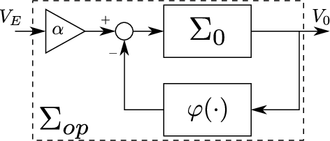
We consider the interconnection of op-amp (8) and linear networks of the form (10) typically in positive or negative feedback, as show in Figure 3.

Passivity is a theory of negative feedback. In order to apply Theorem 2 to positive feedback interconnections, we consider the reverted output and interpret the positive feedback interconnection as negative feedback interconnection of the reverted output:
| (13) |
We note that the network in Figure 4 is strictly -passive from to and strictly -passive from to .

Indeed, define , , and . Then the transfer functions from to reads
| (14) |
whereas the transfer function from to reads
| (15) |
By Theorem 3, is strictly -passive for any rate . On the other hand, is strictly -passive for any rate .
4.3 -Passive circuits
By Theorem 1, multistable circuits that switch among several fixed points may arise from the interconnection of the op-amp with strictly -passive networks. As an illustration, consider the positive feedback of the op-amp with the network in Figure 4.

The network is strictly -passive from to with rate , and takes the role of in Figure 3. The op-amp is -passive with rate . Thus, for
| (16) |
the two systems share a common interval for their rates11 1 (16) requires that the op-amp dynamics is faster than the dynamics of the external network, as usual in applications.. By Theorem 2 the closed loop system in Figure 5 is strictly -passive from to with rate . Theorem 5 guarantees boundedness of the closed-loop trajectories for any constant input . Therefore, Theorem 1 guarantees asymptotic convergence of all trajectories to some fixed point. In particular, taking for simplicity, the closed loop is bistable for
| (17) |
which guarantees the existence of three equilibrium points (two stable nodes and a saddle).
4.4 -Passive circuits
By Theorem 1, oscillatory circuits may arise from the interconnection of the op-amp with strictly -passive networks. As an illustration, consider the negative feedback of the op-amp with the network in Figure 6.

The network admits the state-space representation
The transfer function from to reads
| (18) |
Denoting by the -th pole of and by the magnitude of the real part of the poles of (without loss of generality, we assume ), the network is strictly -passive from to with rate . The network is thus constrained to a negative feedback interconnection, taking the role of in Figure 3. For
| (19) |
the op-amp and the RC network share a common interval for their rates. By Theorem 2 the closed loop system in Figure 6 is thus strictly -passive from to with rate . Theorem 5 guarantees boundedness of the closed loop trajectories for any constant input , thus Theorem 1 guarantees that the trajectories of the four dimensional closed-loop circuit all converge to a simple attractor. For and , has poles , and . Therefore, strict -passivity holds for . For op-amp parameters , , , condition (19) holds. These specific parameters also ensure that the unique fixed point at the origin is unstable. Thus, by Theorem 1, every trajectory converges asymptotically to a limit cycle. The steady-state is an oscillation, as shown in Figure 7.

5 Mixed feedback and modulation
The mixed feedback amplifier is a classical device of nonlinear circuit theory (Chua et al., 1987). It combines positive and negative feedback around an operational amplifier to create nonlinear behaviors. We illustrate this flexibility with the simple system of Figure 8.

The two linear networks correspond to two copies of the network in Figure 4. The behavior of the closed loop is dictated by the interconnection pattern of the switches and . If is closed and is open then the network reduces to the one in Figure 5; the closed loop is -passive. If is open and is closed, then the closed loop is -passive. When both switches are closed, the feedback circuit is not necessarily -passive because the rates of the two networks may not be compatible. In fact, a suitable selection of the network parameters lead to richer behaviors. Take and both closed and define , , and , . With these data, the upper network is strictly -passive from to and the lower network is strictly -passive from to , respectively with rates and . A common rate can be found for , since the op-amp is -passive with rate . In this case, the feedback circuit is -passive, by Theorem 2. In contrast, Theorem 2 cannot be used for because of the absence of a common rate. However, the aggregate transfer function reads
| (20) |
which has positive real part if and only if there exist such that
| (21) | ||||
| (22) |
Indeed,
- 1.
- 2.
is strictly -passive with rate for .
The conditions above reveal that mixed feedback allows for both -passivity and -passivity. The network behavior can be modulated from monostable to oscillatory via parameter variations. Figure 9 shows the degree of -passivity of the closed loop for different values . Indeed, transitions from monostable to oscillatory regimes are obtained by the variation of one of the two resistances.

As a final illustration, we consider parameters , , , , , and . For these parameters in (20) is strictly -passive. When both switches are closed the origin is the only equilibrium point and is unstable. Hence, by Theorems 1 and 5 we conclude the existence of a limit cycle. Figure 10 shows transitions among different behaviors, driven by the switches.

6 Conclusions
We have analyzed basic examples of circuits that switch and oscillate as interconnections of linear circuits and operational amplifiers. The approach builds upon dominance theory and -passivity. The saturated op-amp model guarantees boundedness of trajectories in closed loop and allows for positive and negative feedback interconnections with linear -passive networks. Specific interconnections lead to - and -passive networks, leading to a tractable analysis of bistability and oscillations in possibly high-dimensional models. The stability analysis in this paper is based on solving linear matrix inequalities very much as in the stability analysis of linear systems. Such a computational framework suggests many possible extensions to analyze the performance and robustness of switching and oscillatory circuits in the same way as for linear systems.
References
- Aghannan and Rouchon (2003) Aghannan, N. and Rouchon, P. (2003). An intrinsinc observer for a class of Lagrangian systems. IEEE Transactions on Automatic Control, 48(6).
- Chua et al. (1987) Chua, L.O., Desoer, C.A., and Kuh, E.S. (1987). Linear and nonlinear circuits. Mc-Graw Hill.
- Clayton and Winder (2003) Clayton, G. and Winder, S. (2003). Operational Amplifiers. EDN Series for Design Engineers. Elsevier.
- Forni and Sepulchre (2013) Forni, F. and Sepulchre, R. (2013). On differentially dissipative dynamical systems. In 9th IFAC Symposium on Nonlinear Control Systems, 15–20. Toulouse, France.
- Forni and Sepulchre (2014) Forni, F. and Sepulchre, R. (2014). A differential Lyapunov framework for contraction analysis. IEEE Transactions on Automatic Control, 59(3), 614–628.
- Forni and Sepulchre (2017a) Forni, F. and Sepulchre, R. (2017a). Differential dissipativity theory for dominance analysis. Submitted to IEEE Transactions on Automatic Control, http://arxiv.org/abs/1710.01721.
- Forni et al. (2013) Forni, F., Sepulchre, R., and van der Schaft, A.J. (2013). On differential passivity of physical systems. In 52rd IEEE Conference on Decision and Control, 6580–6585. Florence, Italy.
- Forni and Sepulchre (2017b) Forni, F. and Sepulchre, R. (2017b). A dissipativity theorem for -dominant systems. In 56th IEEE Conference on Decision and Control. Melbourne, Australia.
- Jouffroy and Fossen (2010) Jouffroy, J. and Fossen, T.I. (2010). A tutorial on incremental stability analysis using contraction theory. Modeling, Identification and Control, 31(3), 93–106.
- Karki (2000) Karki, J. (2000). Effect of parasitic capacitance in op amp circuits. Technical Report SLOA013A, Texas Instruments.
- Lohmiller and Slotine (1998) Lohmiller, W. and Slotine, J.J.E. (1998). On contraction analysis for nonlinear systems. Automatica, 34(6), 683–696.
- Miranda-Villatoro et al. (2017) Miranda-Villatoro, F.A., Forni, F., and Sepulchre, R. (2017). Analysis of Lur’e dominant systems in the frequency domain. Submitted to Automatica, http://arxiv.org/abs/1710.01645.
- Miranda-Villatoro et al. (2018) Miranda-Villatoro, F.A., Forni, F., and Sepulchre, R. (2018). Dominance analysis of linear complementarity systems. Submitted to MTNS 2018, http://arxiv.org/abs/1802.00284.
- Noseek (2009) Noseek, J.A. (2009). Circuit elements, modeling and equation formulation. In The Circuits and Filters Handbook: Fundamentals of Circuits and Filters, 13–1, 13–11.
- Pavlov and L (2008) Pavlov, A. and L, M. (2008). Incremental passivity and output regulation. Systems & Control Letters, 57, 400–409.
- Pavlov et al. (2005) Pavlov, A., Van De Wouw, N., and Nijmeijer, H. (2005). Convergent systems: analysis and synthesis. In Control and observer design for nonlinear finite and infinite dimensional systems, 131–146. Springer.
- Stan and Sepulchre (2007) Stan, G.B. and Sepulchre, R. (2007). Analysis of interconnected oscillators by dissipativity theory. IEEE Transactions on Automatic Control, 52(2), 256–270.
- van Der Schaft (2013) van Der Schaft, A.J. (2013). On differential passivity. In 9th IFAC Symposium on Nonlinear Control Systems, 21–25. Toulouse, France.