Owing to their asymptotic characterization, max-stable processes are widely used for modeling spatially-indexed block maxima data. In this section, we briefly summarize the general theory and modeling of max-stable processes in the spatial context, then we extend these processes to the multivariate spatial framework in §3. Let $\{Y_{1}(\mathbf{s}),\ldots,Y_{n}(\mathbf{s})\}_{\mathbf{s}\in\mathcal{S}}$ be independent and identically distributed stochastic processes defined over the spatial region $\mathcal{S}\subset\mathbb{R}^{2}$. If there exist normalization functions ${a_{n}(\mathbf{s})>0}$, ${b_{n}(\mathbf{s})}\in\mathbb{R}$ such that the renormalized process of the pointwise maxima, i.e.,

$$M_{n}(\mathbf{s})=\frac{\max\{{Y_{1}(\mathbf{s}),\ldots,Y_{n}(\mathbf{s})}\}-b_{n}(\mathbf{s})}{a_{n}(\mathbf{s})},\quad\quad\mathbf{s}\in\mathcal{S},$$

(1)

converges in the sense of finite-dimensional distributions to a process $Z^{\star}(\mathbf{s})$ with non-degenerate margins, as $n\rightarrow\infty$, then the limit $Z^{\star}(\mathbf{s})$ is a max-stable process (de Haan, 1984, see, e.g.,). The max-stability of $Z^{\star}(\mathbf{s})$ implies that there exist functions $\alpha_{n}(\mathbf{s})>0$ and $\beta_{n}(\mathbf{s})$ for all $n\in\mathbb{N}$, such that, for each collection of sites $\mathbf{s}_{1},\ldots,\mathbf{s}_{D}\in\mathcal{S}$, $D\in\mathbb{N}$, the finite-dimensional distribution $G(z_{1},\ldots,z_{D})$ of the variables $Z^{\star}(\mathbf{s}_{1}),\ldots,Z^{\star}(\mathbf{s}_{D})$ satisfies

$$G^{n}\{\alpha_{n}(\mathbf{s}_{1})z_{1}+\beta_{n}(\mathbf{s}_{1}),\ldots,\alpha_{n}(\mathbf{s}_{D})z_{D}+\beta_{n}(\mathbf{s}_{D})\}=G(z_{1},\ldots,z_{D}).$$

The limit max-stable process $Z^{\star}(\mathbf{s})$ may be used to represent monthly maxima of daily measurements for a specific air pollutant observed at various locations $\mathbf{s}$ within the study region $\mathcal{S}$. For each location $\mathbf{s}\in\mathcal{S}$, the Extremal Types Theorem (see, e.g., Coles, 2001, Chapter 3) implies that the random variable $Z^{\star}(\mathbf{s})$ follows the generalized extreme-value (GEV) distribution with location $\mu(\mathbf{s})\in\mathbb{R}$, scale $\sigma(\mathbf{s})>0$, and shape $\xi(\mathbf{s})\in\mathbb{R}$ parameters. To disentangle marginal and dependence effects, it is convenient to standardize $Z^{\star}(\mathbf{s})$ as

$$Z(\mathbf{s})=\left\{1+\xi(\mathbf{s})\frac{Z^{\star}(\mathbf{s})-\mu(\mathbf{s})}{\sigma(\mathbf{s})}\right\}^{1/\xi(\mathbf{s})}.$$

(2)

Thus, we obtain a residual, simple, max-stable process $Z(\mathbf{\mathbf{s}})$, which is characterized by unit Fréchet marginal distributions, i.e., $\Pr\{Z(\mathbf{s})\leq z\}=\exp(-1/z)$, $z>0$, for all $\mathbf{s}\in\mathcal{S}$, corresponding to the case $\mu(\mathbf{s})=\sigma(\mathbf{s})=\xi(\mathbf{s})=1$. In practice, data are collected at a finite set of locations, and the joint distribution of $Z(\mathbf{s})$ at $\mathbf{s}_{1},\ldots,\mathbf{s}_{D}\in\mathcal{S}$ is necessarily a multivariate extreme-value distribution that may be expressed as

$$\Pr\{Z(\mathbf{s}_{1})\leq z_{1},\ldots,Z(\mathbf{s}_{D})\leq z_{D}\}=\exp\left\{-V(z_{1},\ldots,z_{D})\right\},\quad z_{1},\ldots,z_{D}>0,$$

(3)

where $V(z_{1},\ldots,z_{D})$ is the associated exponent function containing information about the spatial dependence of the maxima. By max-stability, we can verify that $V$ is homogeneous of order $-1$, i.e., $V(tz_{1},\ldots,tz_{D})=t^{-1}V(z_{1},\ldots,z_{D})$, $t>0$; moreover, because of the unit Fréchet margins in (3), we have $V(z,\infty,\ldots,\infty)=1/z$ for any permutation of the arguments. In particular, in the case of independence between $Z(\mathbf{s}_{1}),\ldots,Z(\mathbf{s}_{D})$ we have $V(z_{1},\ldots,z_{D})=\sum_{d=1}^{D}z_{d}^{-1}$; in the case of perfect positive dependence, we have $V(z_{1},\ldots,z_{D})=\underset{1\leq d\leq D}{\max}z_{d}^{-1}$. The pairwise extremal coefficient $\theta(\mathbf{s}_{i},\mathbf{s}_{j})=V(1,1)\in[1,2]$ (proposed by Smith, 1990; see also Schlather and Tawn, 2003), where $V$ is here restricted to sites $\mathbf{s}_{i}$ and $\mathbf{s}_{j}$, is a measure of the extremal dependence between the variables $Z(\mathbf{s}_{i})$ and $Z(\mathbf{s}_{j})$, $i,j=1,\ldots,D$. Perfect dependence corresponds to $\theta(\mathbf{s}_{i},\mathbf{s}_{j})=1$, and $\theta(\mathbf{s}_{i},\mathbf{s}_{j})=2$ leads to complete independence.

The construction of simple max-stable processes may be described following the spectral characterization of de Haan (1984) (see also Penrose, 1992, and Schlather and Tawn, 2002). Let $W_{i}(\mathbf{s})$, $i\in\mathbb{N}$, be independent realizations of a stochastic process $W(\mathbf{s})$ such that $\textrm{E}[\sup_{\mathbf{s}\in\mathcal{S}}W(\mathbf{s})]<\infty$ with $\textrm{E}[W(\mathbf{s})]=1$ for all $\mathbf{s}\in\mathcal{S}$, and $\zeta_{i}\in\Pi$ be points of the Poisson process $\Pi$ with intensity $\textrm{d}\zeta/\zeta^{2}$ on $\left(0,\infty\right)$. Then, the process constructed as

$$Z(\mathbf{s})=\max_{i\geq 1}\zeta_{i}W_{i}(\mathbf{s}),\qquad\mathbf{s}\in\mathcal{S},$$

(4)

is simple max-stable; its joint distribution function may be written as $\Pr\left\{Z(\mathbf{s})\leq z(\mathbf{s}),\mathbf{s}\in\mathcal{S}\right\}=\exp\left(-\textrm{E}\left[\sup_{\mathbf{s}\in\mathcal{S}}\left\{{W(\mathbf{s})/z(\mathbf{s})}\right\}\right]\right)$, where $z(\mathbf{s})$ is any suitable function defined on $\mathcal{S}$. From (3), it follows that

$$V(z_{1},\ldots,z_{D})=\textrm{E}\left[\sup_{\mathbf{s}\in\mathcal{S}}\left\{{W(\mathbf{s})\over z(\mathbf{s})}\right\}\right].$$

Choosing a different process $W(\mathbf{s})$ will lead to different classes of max-stable processes. Various parametric models have been proposed in the literature. The most well-known in the spatial framework are the Smith (1990), Schlather (2002), Brown-Resnick (Brown and Resnick, 1977; Kabluchko et al., 2009), extremal-$t$ (Nikoloulopoulos et al., 2009; Opitz, 2013), Reich and Shaby (2012), and Tukey (Xu and Genton, 2017) max-stable processes. For comprehensive reviews of the max-stable processes, see, e.g., Davison and Gholamrezaee (2012), Ribatet (2013) and Davison et al. (2018).

One strategy for constructing hierarchical extreme-value models is to assume that the random variables $Z^{\star}(\mathbf{s})$, which are observed at locations $\mathbf{s}_{1},\ldots,\mathbf{s}_{D}\in\mathcal{S}$ and arise in the limit of renormalized maxima in (1), are independent, conditional on some unobserved latent random effects; see Banerjee et al. (2014) for examples of similar hierarchical spatial models in the classical geostatistical literature. The latent Gaussian process approaches of Casson and Coles (1999), Cooley et al. (2007), Davison et al. (2012), Apputhurai and Stephenson (2013), Dyrrdal et al. (2015), and Opitz et al. (2018) aim to accurately capture marginal variation by embedding random effects into the marginal extreme-value parameters, but they lack flexibility to capture strong extremal dependence. In contrast, the Reich–Shaby model (Reich and Shaby, 2012), which is based on latent $\alpha$-stable random effects, captures both marginal and joint spatial properties of extremes. The Reich–Shaby model is the only max-stable process proposed so far that possesses such a convenient hierarchical representation of spatial extremes in terms of some independent latent random effects. By integrating out the $\alpha$-stable random effects, the process resulting from the Reich–Shaby construction is max-stable and its finite-dimensional distributions are a max-mixture of multivariate logistic distributions, with the weights depending on spatial information; this allows the joint dependence structure of the spatial extremes to be described using a convenient hierarchical framework.

The Reich and Shaby (2012) model has been applied to various datasets and studied in different contexts. Reich et al. (2014) used this model to study extremal dependence on temperature time series; Stephenson et al. (2015) analyzed fire danger data from about 17,000 sites using compactly supported kernel functions; and Castruccio et al. (2016) compared the numerical performance of this model estimated using composite likelihood methods.

In this section, we detail the construction and properties of the Reich–Shaby model. Let $U(\mathbf{s})\stackrel{{\scriptstyle\textrm{i.i.d.}}}{{\sim}}\exp(-z^{-1/\alpha})$, $z>0$, $0<\alpha\leq 1$, be a random noise process accounting for small-scale, non-spatial variations in the data (such as measurement errors), called the nugget effect in classical geostatistics. Furthermore, let $\vartheta\left(\mathbf{s}\right)=\left\{\sum_{l=1}^{L}A_{l}\omega_{l}\left(\mathbf{s}\right)^{1/\alpha}\right\}^{\alpha}$, $\mathbf{s}\in\mathcal{S}\subset\mathbb{R}^{2}$, be a smooth spatial process, where the kernels $\omega_{l}\left(\mathbf{s}\right)\geq 0$, $l=1,\ldots,L$, are deterministic spatial profiles (or weights) such that $\sum_{l=1}^{L}\omega_{l}\left(\mathbf{s}\right)=1$ for any location $\mathbf{s}\in\mathcal{S}$, and the $A_{l}$s are independent random amplitudes following the positive $\alpha$-stable distribution, i.e., $A_{l}\stackrel{{\scriptstyle\textrm{i.i.d.}}}{{\sim}}\textrm{PS}(\alpha)$. Although the $\alpha$-stable density function, denoted $f_{\textrm{PS}}(a;\alpha)$, does not have an explicit form for $\alpha\in(0,1)$, its Laplace transform may be expressed as

$$\textrm{E}(e^{-tA_{l}})=\int_{0}^{\infty}e^{-ta}f_{\textrm{PS}}(a;\alpha)\textrm{d}a=e^{-t^{\alpha}},\;t\geq 0.$$

(5)

The max-stable process proposed by Reich and Shaby (2012) with unit Fréchet margins is defined as $Z(\mathbf{s})=U(\mathbf{s})\vartheta(\mathbf{s})$ over the region $\mathcal{S}$. A spatial process with GEV margins can be obtained by inverting the transformation (2). Therefore, a hierarchical model marginalized over the random noise $U(\mathbf{s})$ may be written as

	$\displaystyle Z^{\star}(\mathbf{s})|A_{1},\ldots,A_{L}$	$\displaystyle\stackrel{{\scriptstyle\textrm{ind}}}{{\sim}}\textrm{GEV}\{\mu^{\star}(\mathbf{s}),\sigma^{\star}(\mathbf{s}),\xi^{\star}(\mathbf{s})\},$
	$\displaystyle A_{1},\ldots,A_{L}$	$\displaystyle\stackrel{{\scriptstyle\textrm{i.i.d.}}}{{\sim}}\mathbf{\textrm{PS}}(\alpha),$

where $\mu^{\star}(\mathbf{s})=\mu(\mathbf{s})+\sigma(\mathbf{s})/\xi(\mathbf{s})\{\vartheta(\mathbf{s})^{\xi(\mathbf{s})}-1\},\sigma^{\star}(\mathbf{s})=\alpha\sigma(\mathbf{s})\vartheta(\mathbf{s})^{\xi(\mathbf{s})}$, and $\xi^{\star}(\mathbf{s})=\alpha\xi(\mathbf{s})$. The latent random effects $A_{1},\ldots,A_{L}$ induce max-stable spatial dependence; this specific hierarchical construction ensures that the joint distribution of $Z^{\star}(\mathbf{s})$ is max-stable with ${\rm GEV}\{\mu(\mathbf{s}),\sigma(\mathbf{s}),\xi(\mathbf{s})\}$ margins when the random effects $A_{1},\ldots,A_{L}$ are integrated out.

Furthermore, the residual unit Fréchet spatial process $Z(\mathbf{s})$, observed at $D$ locations $\mathbf{s}_{1},\ldots,\mathbf{s}_{D}$, is distributed according to (3) with the exponent function

$$V(z_{1},...,z_{D})=\sum_{l=1}^{L}\left[\sum_{d=1}^{D}\left\{{z_{d}\over\omega_{l}(\mathbf{s}_{d})}\right\}^{-1/\alpha}\right]^{\alpha},\quad\quad z_{1},\ldots,z_{D}>0,$$

(6)

which corresponds to a max-mixture of independent random vectors $(Z_{l;1},\ldots,Z_{l;D})^{\top}$, $l=1,\ldots,L$, that are distributed according to the logistic multivariate extreme-value distribution (Gumbel, 1960), i.e., $\{Z(\mathbf{s}_{1}),\ldots,Z(\mathbf{s}_{D})\}^{\top}=\left\{\max_{l=1,\ldots,L}\omega_{l}(\mathbf{s}_{1})Z_{l;1},\ldots,\max_{l=1,\ldots,L}\omega_{l}(\mathbf{s}_{D})Z_{l;D}\right\}^{\top}$. This makes the link with the general spectral representation (4) (Reich and Shaby, 2012, see also). Because of the asymmetry introduced by the weights $\omega_{l}(\mathbf{s})$, the model (6) is closely related to the asymmetric logistic model introduced by Tawn (1990). Although other kernels are possible, Reich and Shaby (2012) proposed using the isotropic Gaussian density function

$$g_{l}(\mathbf{s})={1\over 2\pi\tau^{2}}\exp\left\{-{1\over 2\tau^{2}}(\mathbf{s}-\mathbf{v}_{l})^{\top}(\mathbf{s}-\mathbf{v}_{l})\right\},\quad l=1,\ldots,L,$$

(7)

with a bandwidth (i.e., spatial range parameter) $\tau>0$ and fixed spatial knots $\mathbf{v}_{1},\ldots,\mathbf{v}_{L}$ distributed over the domain $\mathcal{S}$. We rescale the kernels to ensure that they sum to one at each location, i.e., $\omega_{l}(\mathbf{s})=g_{l}(\mathbf{s})\left\{\sum_{l=1}^{L}g_{l}(\mathbf{s})\right\}^{-1}$, so that the margins of $Z(\mathbf{s})$ are unit Fréchet.

In the following section, we explain how to extend this hierarchical max-stable construction for the joint modeling of maxima from multiple variables observed over space.

We generalize the univariate Reich–Shaby process, described in §2.3, in order to capture the complex spatial and cross-dependence structures among the maxima of several variables observed at multiple sites. In our proposed multivariate spatial process, the univariate spatial margins follow the Reich–Shaby model, and interact with each other by assuming a nested tree-based structure for their latent $\alpha$-stable random effects.

For illustration purposes, we first define the two-layer nested multivariate max-stable process, and then gradually extend it to multilayer tree structures. Analogously to the hierarchical construction detailed in §2.3, for each $k=1,\ldots,K$, let $U_{k}(\mathbf{s})\stackrel{{\scriptstyle\textrm{i.i.d.}}}{{\sim}}\exp\{-z^{-1/(\alpha_{k}\alpha_{0})}\}$, $z>0$, denote a random Fréchet noise process controlled by the product of the two parameters $\alpha_{k},\alpha_{0}\in(0,1]$; and let $\vartheta_{k}(\mathbf{s})=\left\{\sum_{l=1}^{L}A_{k;l}A_{0;l}^{1/\alpha_{k}}\omega_{k;l}(\mathbf{s})^{1/(\alpha_{k}\alpha_{0})}\right\}^{\alpha_{k}\alpha_{0}}$ be a smooth spatial process, where the terms $\omega_{k;l}\left(\mathbf{s}\right)\geq 0$ are $L$ kernel basis functions representing deterministic weights, such that $\sum_{l=1}^{L}\omega_{k;l}\left(\mathbf{s}\right)=1$ for any $\mathbf{s}\in\mathcal{S}$, and the variables $A_{k;l}$ and $A_{0;l}$, $l=1,\ldots,L$, are mutually independent (across both $k=1,\ldots,K$ and $l=1,\ldots,L$) $\alpha$-stable variables with parameters $\alpha_{k}$ and $\alpha_{0}$, respectively. Thus, $A_{k;l}\stackrel{{\scriptstyle\textrm{i.i.d.}}}{{\sim}}\textrm{PS}(\alpha_{k})\mathchoice{\mathrel{\hbox to0.0pt{$\displaystyle\perp$\hss}\mkern 2.0mu{\displaystyle\perp}}}{\mathrel{\hbox to0.0pt{$\textstyle\perp$\hss}\mkern 2.0mu{\textstyle\perp}}}{\mathrel{\hbox to0.0pt{$\scriptstyle\perp$\hss}\mkern 2.0mu{\scriptstyle\perp}}}{\mathrel{\hbox to0.0pt{$\scriptscriptstyle\perp$\hss}\mkern 2.0mu{\scriptscriptstyle\perp}}}A_{0;l}\stackrel{{\scriptstyle\textrm{i.i.d.}}}{{\sim}}\textrm{PS}(\alpha_{0})$. Using the Laplace transform (5), we can show that $A_{k;l}A_{0;l}^{1/\alpha_{k}}$ follows an $\alpha$-stable distribution with the parameter $\alpha_{k}\alpha_{0}$; therefore, each process defined as $Z_{k}(\mathbf{s})=U_{k}(\mathbf{s})\vartheta_{k}(\mathbf{s})$ ($k=1,\ldots,K$) is a univariate Reich–Shaby process defined over the region $\mathcal{S}\subset\mathbb{R}^{2}$, with the dependence parameter $\alpha_{k}\alpha_{0}$, kernels $\omega_{k;l}(\mathbf{s})$, $l=1,\ldots,L$, and unit Fréchet margins. Cross-dependence among these marginal processes is induced by their shared latent variables $A_{0;1},\ldots,A_{0;L}$. Similarly to the Reich–Shaby model, we obtain a spatial process $Z_{k}^{\star}(\mathbf{s})$ with GEV margins by inverting the transformation (2). In this way, we write the hierarchical model marginalized over the random noise $U_{k}(\mathbf{s})$ as

	$\displaystyle Z_{k}^{\star}(\mathbf{s})\mid\{A_{0;l},A_{k;l}\}_{l=1}^{L}$	$\displaystyle\stackrel{{\scriptstyle\textrm{ind}}}{{\sim}}\textrm{GEV}\{\mu_{k}^{\star}(\mathbf{s}),\sigma_{k}^{\star}(\mathbf{s}),\xi_{k}^{\star}(\mathbf{s})\},$
	$\displaystyle A_{k;l}\stackrel{{\scriptstyle\textrm{i.i.d.}}}{{\sim}}\mathbf{\textrm{PS}}(\alpha_{k})$	$\displaystyle\mathchoice{\mathrel{\hbox to0.0pt{$\displaystyle\perp$\hss}\mkern 2.0mu{\displaystyle\perp}}}{\mathrel{\hbox to0.0pt{$\textstyle\perp$\hss}\mkern 2.0mu{\textstyle\perp}}}{\mathrel{\hbox to0.0pt{$\scriptstyle\perp$\hss}\mkern 2.0mu{\scriptstyle\perp}}}{\mathrel{\hbox to0.0pt{$\scriptscriptstyle\perp$\hss}\mkern 2.0mu{\scriptscriptstyle\perp}}}A_{0;l}\stackrel{{\scriptstyle\textrm{i.i.d.}}}{{\sim}}\mathbf{\textrm{PS}}(\alpha_{0}),\quad l=1,\ldots,L$

for $k=1,\ldots,K$, where $\mu_{k}^{\star}(\mathbf{s})=\mu_{k}(\mathbf{s})+\sigma_{k}(\mathbf{s})/\xi_{k}(\mathbf{s})\{\vartheta_{k}(\mathbf{s})^{\xi_{k}(\mathbf{s})}-1\},\sigma_{k}^{\star}(\mathbf{s})=\alpha_{k}\alpha_{0}\sigma_{k}(\mathbf{s})\vartheta_{k}(\mathbf{s})^{\xi_{k}(\mathbf{s})}$, and $\xi_{k}^{\star}(\mathbf{s})=\alpha_{k}\alpha_{0}\xi_{k}(\mathbf{s})$. Then, we combine the residual univariate processes $Z_{k}(\mathbf{s}),\;k=1,\ldots,K$, into the multivariate max-stable process $\mathbf{Z}(\mathbf{s})=\{Z_{1}(\mathbf{s}),\ldots,Z_{K}(\mathbf{s})\}^{\top}$, whose finite-dimensional distributions at $D$ locations $\mathbf{s}_{1},\ldots,\mathbf{s}_{D}$ are expressed as (3) in terms of the exponent function

$$V(\mathbf{z}_{1},...,\mathbf{z}_{K})=\sum_{l=1}^{L}\left(\sum_{k=1}^{K}\left[\sum_{d=1}^{D}\left\{{z_{k;d}\over\omega_{k;l}(\mathbf{s}_{d})}\right\}^{-1/(\alpha_{k}\alpha_{0})}\right]^{\alpha_{k}}\right)^{\alpha_{0}},\quad z_{k;d}>0\quad\mbox{for all $k,d$.}$$

(8)

In (8), $\mathbf{z}_{k}=(z_{k;1},\ldots,z_{k;D})^{\top}$ denotes the vector containing the maxima of the $k$th variable observed at $D$ locations, while the parameters $0<\alpha_{k},\alpha_{0}\leq 1$ ($k=1,\ldots,K$) control the spatial and cross-dependence structures. The proof of (8) is provided in Appendix A. Model (8) corresponds to a max-mixture of $L$ independent nested logistic max-stable distributions (Tawn, 1990; Stephenson, 2003), with the weights $\omega_{k;l}(\mathbf{s})$ introducing spatial asymmetries. This nested cross-dependence structure, represented by a simple tree in Figure 1, assumes that all the univariate processes are exchangeable. In the following, we refer to the max-stable process $\mathbf{Z}(\mathbf{s})$ with the exponent function (8) as a two-layer nested multivariate max-stable process.

The exchangeability of such two-layer processes is not always realistic, but we overcome this limitation by generalizing the construction principle above to multilayer, partially exchangeable, tree structures based on additional nested $\alpha$-stable random effects. Because of the similarities in the ways these complex models are built, we now briefly illustrate the characterization of a three-layer nested max-stable process. We define $T$ exchangeable clusters, each comprised of $K_{t}$ ($t=1,\ldots,T$) max-stable processes. Thus, we have a total of $K=\sum_{t=1}^{T}K_{t}$ spatial processes. For each cluster $t=1,\ldots,T$ and variable $k=1,\ldots,K_{t}$, let $U_{t;k}(\mathbf{s})\stackrel{{\scriptstyle\textrm{i.i.d.}}}{{\sim}}\exp\{-z^{-1/(\alpha_{t;k}\alpha_{t}\alpha_{0})}\}$, $z>0$, be a random Fréchet noise process, and let $\vartheta_{t;k}(\mathbf{s})=\left\{\sum_{l=1}^{L}A_{{t;k};l}A_{t;l}^{1/\alpha_{t;k}}A_{0;l}^{1/(\alpha_{t;k}\alpha_{t})}\omega_{t;k;l}(\mathbf{s})^{1/(\alpha_{t;k}\alpha_{t}\alpha_{0})}\right\}^{\alpha_{t;k}\alpha_{t}\alpha_{0}}$ be a smooth spatial process, where $\alpha_{t;k},\alpha_{t},\alpha_{0}\in(0,1]$ are dependence parameters, $\omega_{t;k;l}\left(\mathbf{s}\right)\geq 0$ denote deterministic weights such that $\sum_{l=1}^{L}\omega_{t;k;l}\left(\mathbf{s}\right)=1$, for any $\mathbf{s}\in\mathcal{S}$, and $A_{t;k;l}\stackrel{{\scriptstyle\textrm{i.i.d.}}}{{\sim}}\textrm{PS}(\alpha_{t;k})\mathchoice{\mathrel{\hbox to0.0pt{$\displaystyle\perp$\hss}\mkern 2.0mu{\displaystyle\perp}}}{\mathrel{\hbox to0.0pt{$\textstyle\perp$\hss}\mkern 2.0mu{\textstyle\perp}}}{\mathrel{\hbox to0.0pt{$\scriptstyle\perp$\hss}\mkern 2.0mu{\scriptstyle\perp}}}{\mathrel{\hbox to0.0pt{$\scriptscriptstyle\perp$\hss}\mkern 2.0mu{\scriptscriptstyle\perp}}}A_{t;l}\stackrel{{\scriptstyle\textrm{i.i.d.}}}{{\sim}}\textrm{PS}(\alpha_{t})\mathchoice{\mathrel{\hbox to0.0pt{$\displaystyle\perp$\hss}\mkern 2.0mu{\displaystyle\perp}}}{\mathrel{\hbox to0.0pt{$\textstyle\perp$\hss}\mkern 2.0mu{\textstyle\perp}}}{\mathrel{\hbox to0.0pt{$\scriptstyle\perp$\hss}\mkern 2.0mu{\scriptstyle\perp}}}{\mathrel{\hbox to0.0pt{$\scriptscriptstyle\perp$\hss}\mkern 2.0mu{\scriptscriptstyle\perp}}}A_{0;l}\stackrel{{\scriptstyle\textrm{i.i.d.}}}{{\sim}}\textrm{PS}(\alpha_{0})$ are mutually independent latent $\alpha$-stable random amplitudes. Then, we set $Z_{t;k}(\mathbf{s})=U_{t;k}(\mathbf{s})\vartheta_{t;k}(\mathbf{s})$, and define the nested multivariate max-stable process with unit Fréchet margins as $\mathbf{Z}(\mathbf{s})=\{\mathbf{Z}_{1}^{\top}(\mathbf{s}),\ldots,\mathbf{Z}_{T}^{\top}(\mathbf{s})\}^{\top}$ with $\mathbf{Z}_{t}(\mathbf{s})=\{Z_{t;1}(\mathbf{s}),\ldots,Z_{t;K_{t}}(\mathbf{s})\}^{\top}$, $t=1,\ldots,T$. Analogously to (8), the finite-dimensional distributions of $\mathbf{Z}(\mathbf{s})$ observed at $D$ locations $\mathbf{s}_{1},\ldots,\mathbf{s}_{D}\in\mathcal{S}$ may be written as (3) with the exponent function

$$V(\mathbf{z}_{1},...,\mathbf{z}_{T})=\sum_{l=1}^{L}\left\{\sum_{t=1}^{T}\left(\sum_{k=1}^{K_{t}}\left[\sum_{d=1}^{D}\left\{{z_{t;k;d}\over\omega_{t;k;l}(\mathbf{s}_{d})}\right\}^{-1/(\alpha_{t;k}\alpha_{t}\alpha_{0})}\right]^{\alpha_{t;k}}\right)^{\alpha_{t}}\right\}^{\alpha_{0}},\;\;z_{t;k;d}>0\quad\mbox{for all $t,k,d$,}$$

(9)

where $\mathbf{z}_{t}=(\mathbf{z}_{t;1}^{\top},\ldots,\mathbf{z}_{t;K_{t}}^{\top})^{\top}$ and $\mathbf{z}_{t;k}=(z_{t;k;1},\ldots,z_{t;k;D})^{\top}$, $t=1,\ldots,T$, $k=1,\ldots,K_{t}$. The proof of (9) is provided in Appendix A. As illustrated in Figure 2, the multivariate process $\mathbf{Z}(\mathbf{s})$ with (9) is represented graphically using a tree, whereby the terminal nodes represent the marginal max-stable processes and the upper nodes describe the cross-dependence relationships among the processes. When $T=1$ and $\alpha_{1;k}\alpha_{1}\equiv\alpha_{k}$, (9) reduces to the two-layer case in (8). Hence, (9) provides more flexibility than (8) for representing complex cross-dependence structures, and we call it a three-layer nested multivariate max-stable process. Using the inverse mapping stemming from (2), we obtain a three-layer nested multivariate max-stable process with arbitrary GEV margins and a hierarchical formulation:

	$\displaystyle Z_{t;k}^{\star}(\mathbf{s})\mid\{A_{0;l},A_{t;l},A_{t;k;l}\}_{l=1}^{L}$	$\displaystyle\stackrel{{\scriptstyle\textrm{ind}}}{{\sim}}\textrm{GEV}\{\mu_{t;k}^{\star}(\mathbf{s}),\sigma_{t;k}^{\star}(\mathbf{s}),\xi_{t;k}^{\star}(\mathbf{s})\},$		(10)
	$\displaystyle A_{t;k;l}\stackrel{{\scriptstyle\textrm{i.i.d.}}}{{\sim}}\mathbf{\textrm{PS}}(\alpha_{t;k})\mathchoice{\mathrel{\hbox to0.0pt{$\displaystyle\perp$\hss}\mkern 2.0mu{\displaystyle\perp}}}{\mathrel{\hbox to0.0pt{$\textstyle\perp$\hss}\mkern 2.0mu{\textstyle\perp}}}{\mathrel{\hbox to0.0pt{$\scriptstyle\perp$\hss}\mkern 2.0mu{\scriptstyle\perp}}}{\mathrel{\hbox to0.0pt{$\scriptscriptstyle\perp$\hss}\mkern 2.0mu{\scriptscriptstyle\perp}}}A_{t;l}$	$\displaystyle\stackrel{{\scriptstyle\textrm{i.i.d.}}}{{\sim}}\mathbf{\textrm{PS}}(\alpha_{t})\mathchoice{\mathrel{\hbox to0.0pt{$\displaystyle\perp$\hss}\mkern 2.0mu{\displaystyle\perp}}}{\mathrel{\hbox to0.0pt{$\textstyle\perp$\hss}\mkern 2.0mu{\textstyle\perp}}}{\mathrel{\hbox to0.0pt{$\scriptstyle\perp$\hss}\mkern 2.0mu{\scriptstyle\perp}}}{\mathrel{\hbox to0.0pt{$\scriptscriptstyle\perp$\hss}\mkern 2.0mu{\scriptscriptstyle\perp}}}A_{0;l}\stackrel{{\scriptstyle\textrm{i.i.d.}}}{{\sim}}\mathbf{\textrm{PS}}(\alpha_{0}),\quad l=1,\ldots,L,$

where the marginal parameters satisfy $\mu_{t;k}^{\star}(\mathbf{s})=\mu_{t;k}(\mathbf{s})+\sigma_{t;k}(\mathbf{s})/\xi_{t;k}(\mathbf{s})\{\vartheta_{t;k}(\mathbf{s})^{\xi_{t;k}(\mathbf{s})}-1\},\sigma_{t;k}^{\star}(\mathbf{s})=\alpha_{0}\alpha_{t}\alpha_{t;k}\sigma_{t;k}(\mathbf{s})\vartheta_{t;k}(\mathbf{s})^{\xi_{t;k}(\mathbf{s})}$, and $\xi_{t;k}^{\star}(\mathbf{s})=\alpha_{0}\alpha_{t}\alpha_{t;k}\xi_{t;k}(\mathbf{s})$. By integrating out the latent $\alpha$-stable random effects, the resulting process $Z_{t;k}^{\star}(\mathbf{s})$ is max-stable and has GEV margins with parameters $\mu_{t;k}(\mathbf{s})$, $\sigma_{t;k}(\mathbf{s})$, and $\xi_{t;k}(\mathbf{s})$.

We now investigate the dependence properties of nested multivariate max-stable processes. In a three-layer multivariate max-stable model (see §3.1), each marginal process $Z_{t;k}(\mathbf{s})$, $t=1,\ldots,T$, $k=1,\ldots,K_{t},$ is a Reich–Shaby process with unit Fréchet margins; therefore, it inherits its spatial dependence properties, which were studied in depth by Reich and Shaby (2012). The product $\alpha_{t;k}\alpha_{t}\alpha_{0}$ plays the role of the dependence parameter $\alpha$ in (6) and acts as a mediator between the noise component $U_{t;k}(\mathbf{s})$ and the smooth spatial process $\vartheta_{t;k}(\mathbf{s})$. Below, we describe the cross-dependence properties of our new multivariate spatial model.

Similar to Reich and Shaby (2012), we propose using the Gaussian kernel (7) with a different bandwidth $\tau_{t;k}>0$ for each marginal process, and the spatial knots $\mathbf{v}_{1},\ldots,\mathbf{v}_{L}\in\mathcal{S}$ are fixed on a regular grid. Again, we rescale, the kernels to ensure that they sum to one at each location, i.e., $\omega_{t;k;l}(\mathbf{s})=g_{t;k;l}(\mathbf{s})\{\sum_{l=1}^{L}g_{t;k;l}(\mathbf{s})\}^{-1}$, $t=1,\ldots,T$, $k=1,\ldots,K_{t}$, with $g_{t;k;l}$ defined similarly to $g_{l}$ in (7). In practice, we must choose a number of knots $L$ that balances computational feasibility with modeling accuracy. A too small $L$ might not be realistic and could affect subsequent inferences by artificially creating a non-stationary process (Castruccio et al., 2016), whereas a too large $L$ would significantly increase the computational burden. Reich and Shaby (2012) suggested fixing the number of knots, $L$, such that the grid spacing is approximately equal to or smaller than the kernel bandwidth $\tau_{t;k}$.

To understand the cross-dependence structure of (9) and the meaning of its parameters, we consider the product of the dependence parameters along a specific path through the underlying tree. As mentioned above, $\alpha_{t;k}\alpha_{t}\alpha_{0}$ governs the amount of noise attributed to the univariate Reich–Shaby process in the corresponding terminal node on a given path; in contrast, $\alpha_{t}\alpha_{0}$ controls the cross-dependence among the variables belonging to the same cluster $t=1,\ldots,T$. The cross-dependence among variables belonging to distinct clusters is controlled by $\alpha_{0}$. Since $\alpha_{t}\alpha_{0}\leq\alpha_{0}$, the intra-cluster cross-dependence is always stronger than the inter-cluster cross-dependence.

For model (9), the pairwise extremal coefficient $\theta\{\mathbf{s}_{i},\mathbf{s}_{j};(t_{1};k_{1}),(t_{2};k_{2})\}\in[1,2]$ (see §2.1) summarizes the strength of dependence between each pair of variables $\{Z_{t_{1};k_{1}}(\mathbf{s}_{i}),Z_{t_{2};k_{2}}(\mathbf{s}_{j})\}^{\top}$, with $t_{1},t_{2}=1,\ldots,T$, $k_{1}=1,\ldots,K_{t_{1}}$, $k_{2}=1,\ldots,K_{t_{2}}$. The variables $Z_{t_{1};k_{1}}(\mathbf{s}_{i})$ (process $k_{1}$ in cluster $t_{1}$ observed at location $\mathbf{s}_{i}$) and $Z_{t_{2};k_{2}}(\mathbf{s}_{j})$ (process $k_{2}$ in cluster $t_{2}$ observed at location $\mathbf{s}_{j}$) are perfectly dependent when $\theta\{\mathbf{s}_{i},\mathbf{s}_{j};(t_{1};k_{1}),(t_{2};k_{2})\}=1$, and completely independent when $\theta\{\mathbf{s}_{i},\mathbf{s}_{j};(t_{1};k_{1}),(t_{2};k_{2})\}=2$. The dependence strength increases monotonically as the value of the extremal coefficient approaches unity. Writing $\theta\{\mathbf{s}_{i},\mathbf{s}_{j};(t_{1};k_{1}),(t_{2};k_{2})\}\equiv\theta(\mathbf{s}_{i},\mathbf{s}_{j})$ for simplicity, we distinguish three cases from (9):

$$\theta(\mathbf{s}_{i},\mathbf{s}_{j})=\left\{\begin{array}[]{ll}\sum_{l=1}^{L}\left\{\omega_{t;k;l}(\mathbf{s}_{i})^{1/(\alpha_{t;k}\alpha_{t}\alpha_{0})}+\omega_{t;k;l}(\mathbf{s}_{j})^{1/(\alpha_{t;k}\alpha_{t}\alpha_{0})}\right\}^{\alpha_{t;k}\alpha_{t}\alpha_{0}},&t_{1}=t_{2}=t,\;k_{1}=k_{2}=k,\\ \sum_{l=1}^{L}\left\{\omega_{t;k_{1};l}(\mathbf{s}_{i})^{1/(\alpha_{t}\alpha_{0})}+\omega_{t;k_{2};l}(\mathbf{s}_{j})^{1/(\alpha_{t}\alpha_{0})}\right\}^{\alpha_{t}\alpha_{0}},&t_{1}=t_{2}=t,\;k_{1}\neq k_{2},\\ \sum_{l=1}^{L}\left\{\omega_{t_{1};k_{1};l}(\mathbf{s}_{i})^{1/\alpha_{0}}+\omega_{t_{2};k_{2};l}(\mathbf{s}_{j})^{1/\alpha_{0}}\right\}^{\alpha_{0}},&t_{1}\neq t_{2},\;k_{1}\neq k_{2}.\\ \end{array}\right.$$

(11)

Hence, as the two sites get closer to each other, i.e., as $\mathbf{s}_{i}\to\mathbf{s}_{j}$, the cross-extremal coefficient reduces to

$$\theta(\mathbf{s}_{i},\mathbf{s}_{j})\to\left\{\begin{array}[]{ll}2^{\alpha_{t;k}\alpha_{t}\alpha_{0}},&t_{1}=t_{2}=t,\;k_{1}=k_{2}=k,\\ 2^{\alpha_{t}\alpha_{0}},&t_{1}=t_{2}=t,\;k_{1}\neq k_{2},\\ 2^{\alpha_{0}},&t_{1}\neq t_{2},\;k_{1}\neq k_{2}.\\ \end{array}\right.$$

(12)

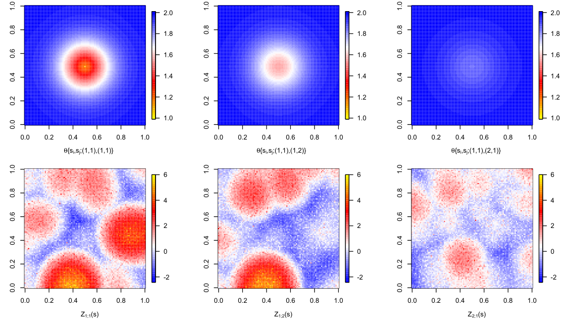
Equation (12) clearly confirms that intra-cluster cross-dependence is stronger than inter-cluster cross-dependence. Moreover, the nugget effect is evident when we notice that $2^{\alpha_{0}}>1$ for all values of $\alpha_{0}\in(0,1]$. Figure 3 illustrates these pairwise dependence properties and shows realizations of the three-layer nested max-stable model with exponent function (9) and the underlying tree structure displayed in Figure 2, for specific values of the dependence parameters. The pairwise extremal coefficients shown in the top row confirm that spatial dependence for each individual process is stronger than cross-dependence, and that intra-cluster cross-dependence is stronger than inter-cluster cross-dependence. The realizations displayed in the bottom row show that strong cross-dependence between two distinct variables may result in co-localized spatial extremes.

Parameter estimation for this type of model may be performed within a Bayesian framework by implementing a standard Metropolis–Hastings Markov chain Monte Carlo (MH-MCMC) algorithm (Hastings, 1970), which takes advantage of the hierarchical formulation (10); see, e.g., Reich and Shaby (2012) and Apputhurai and Stephenson (2013) for applications to precipitation extremes. In the Supplementary Material, we detail the implementation of the MH-MCMC algorithm, which draws approximate samples from the posterior distributions of the dependence parameters $\alpha_{t;k},\alpha_{t},\alpha_{0}$, and $\tau_{t;k}$, where $t=1,\ldots,T$, $k=1,\ldots,K_{t}$, for the nested max-stable model (9). Essentially, the dependence parameters $\alpha_{t;k},\alpha_{t},\alpha_{0}$, and $\tau_{t;k}$ are updated successively (one by one) at each iteration $r=1,\ldots,R$ of the algorithm by generating candidate values $\alpha^{(\textrm{c})}_{t;k},\alpha^{(\textrm{c})}_{t},\alpha^{(\textrm{c})}_{0}$, and $\tau^{(\textrm{c})}_{t;k}$, computing the corresponding candidate process $\vartheta^{(\textrm{c})}_{t;k}$, and finally accepting such candidate values with a certain probability that ensures theoretical convergence of the Markov chain to its stationary posterior distribution. For simplicity, we assume here that the prior distributions of the parameters $\alpha_{t;k},\alpha_{t}$, and $\alpha_{0}$ are non-informative ${\rm Unif}(0,1)$, and that the range parameters $\tau_{t;k}$ have prior distribution equal to $0.5h_{\max}\times{\rm Beta}(2,5)$ as suggested by Sebille et al. (2016), where $h_{\max}$ denotes the maximum distance between stations (representing the “diameter” of the region of study). This slightly informative prior distribution guides and stabilizes the estimation of the range parameters, whose posterior distribution can sometimes be very right-skewed, but it should not have an important impact on the estimated model for a large $D$, i.e., when there are many monitoring stations.

In order to verify the performance of the MH-MCMC algorithm implemented for the nested multivariate max-stable process proposed in §3, we conduct a simulation study and explore some diagnostics of the output. The chosen simulation design conforms to the experiments reported by Reich and Shaby (2012) for each univariate process $Z_{t;k}(\mathbf{s})$, $t=1,\ldots,T$, $k=1,\ldots,K_{t}$, so here we focus on testing the accuracy of the estimates for the cross-dependence parameters $\alpha_{t;k}$, $\alpha_{t}$, and $\alpha_{0}$. We generate data from the nested max-stable models with two nesting layers (8) and three nesting layers (9), using the tree structures $T_{1}$ and $T_{2}$, respectively, represented in Figure 4, with $N=20$ independent time replicates. We consider different values for the dependence parameters $\alpha_{t;k},\alpha_{t}$, and $\alpha_{0}$, fix the bandwidth $\tau_{t;k}=3$ in each individual process, and assign the marginal parameters $\mu_{t;k}(\mathbf{s})=\sigma_{t;k}(\mathbf{s})=\xi_{t;k}(\mathbf{s})=1$, corresponding to the unit Fréchet case. The data are simulated on a $5\times 5$ regular grid (i.e., $D=25$) covering the domain $\mathcal{S}=[0,6]\times[0,6]$, with Gaussian kernels centered on the same grid points. The MH-MCMC output is (partly) represented in Figure 5 for the two-layer case and in Figure 6 for the three-layer case. We performed $R=5\times 10^{5}$ iterations for the two-layer case and $R=10^{6}$ iterations for the three-layer case, then thinned the resulting chains by a factor $2500$ after removing a burn-in of $R/5$ iterations. By integrating C++ code in R using the package Rcpp, the computational time was less than two days for each experiment.

The trace plots of both model outputs suggest that the resulting chains are fairly stationary for all parameters. Moreover, the autocorrelation functions indicate that the subchains show relatively good mixing properties after thinning, although the effective sample sizes suggest that the parameters controlling the upper part of the hierarchy are more difficult to estimate. For example, the parameter $\alpha_{0}$, which mostly impacts the inter-cluster dependence, indeed appears to be the most strongly auto-correlated. Figure 7 shows that the MH-MCMC algorithm produces similar results from different starting values, which strongly confirms that the Markov chain indeed converges to its stationary distribution. Overall, the posterior medians of the dependence parameters coincide with the true values, indicating that our model captures both the spatial and cross-dependence structures governing the joint behavior of these max-stable processes quite well.

High concentrations of pollution in the air can harm the human body. Current methods for assessing air pollution dangers typically consider each pollutant separately, ignoring the heightened threat of exposure to multiple air pollutants. In order to inform the public and government administrations, the US Environmental Protection Agency (EPA) and other international organizations are moving towards a multi-pollutant approach for quantifying health risks of air pollution. In this work, we investigate the extremal dependence among air pollutants and temperature jointly across space. The data consist of daily observations of carbon monoxide (CO), nitric oxide (NO), nitrogen dioxide (NO₂), ozone (O₃), and temperature (T), collected from January 2006 to December 2015, at a number of sites in the area of Los Angeles, CA; see Figure 8. A similar study was conducted by Vettori et al. (2017), who analyzed the extremal dependence between air pollutants and meteorological parameters at several sites in California separately, thereby ignoring their spatial dependence. Here, we use our new methodology based on nested multivariate max-stable processes to characterize the spatial and cross-dependence structures among these variables of interest.

We start by modeling the non-stationary marginal effects from the monthly maxima of each pollutant and meteorological parameter through linear regression, including trend and seasonality terms, and then we standardize these maxima data to a common unit Fréchet scale in order to analyze their complex multivariate dependence structure. By using the tree mixture MCMC (TM-MCMC) algorithm introduced by Vettori et al. (2017) for purely multivariate (i.e., non-spatial) data, we investigate plausible multivariate cross-dependence structures for each site separately. By exploiting reversible jump MCMC and the simple tree-based representation of the nested logistic distribution, this algorithm samples from the posterior distribution of the parameters and the tree itself. We apply the TM-MCMC algorithm with $R=5000$ iterations and a thinning factor of $5$ to the stationary, standardized, monthly maxima time series of the variables CO, NO, NO₂, O₃, and T separately for each site displayed in Figure 8. The most likely dependence structures identified by the TM-MCMC algorithm and the associated posterior probabilities are presented in Figure 9. The tree structures that appear most often across the chains are trees A, B, and C. We find that extreme concentrations of CO and NO are consistently grouped together in the same cluster by trees A, B and C. Moreover, the extreme concentrations of NO₂ are grouped with extreme concentrations of O₃ and high temperatures in tree B, and with extreme concentrations of CO and NO in tree C.

In Figure 10, we fit the three-layer nested multivariate max-stable model with the tree dependence structures A, B, and C; the posterior medians are reported in each node. The estimated parameters $\alpha_{0}$ take values close to $0.9$ in all three trees, indicating that the extreme concentrations of CO and NO are weakly related to the extreme concentrations of NO₂ and O₃ and to high temperatures across the Los Angeles area. Spatial dependence is strongest between the pollutants CO and NO in tree A and between CO and NO₂ in the case of tree C, whereas dependence among NO₂, O₃, and high temperature is strongest in the case of tree B. Figure 11 compares the empirical estimates of the pairwise extremal coefficients (see Smith, 1990 and §2.1) with the pairwise extremal coefficients computed from the fitted nested multivariate max-stable model (11), using the dependence structure of tree B. Generally, model-based estimates are fairly similar to their empirical counterparts (given that the empirical estimates are highly variable), suggesting that the fitted model is reasonable and adequately captures the complex spatial cross-dependence structure of extremes in our dataset. Considering more complex tree structures might further improve the fit. As expected, the pairwise extremal coefficient estimates computed for individual variables seem to increase with the distance between sites. Moreover, both the empirical and model-based pairwise cross-extremal coefficient estimates indicate a moderate dependence strength between variables belonging to the same cluster, such as CO and NO, O₃ and NO₂, or O₃ and T, regardless of the distance between sites, whereas the variables belonging to different clusters, such as O₃ and CO or O₃ and NO, appear to be almost independent at any distances.

The US EPA typically uses the Air Quality Index (AQI) to communicate air pollution risks to the public. In order to illustrate the impacts of neglecting spatial and cross-dependence structures on the AQI return level estimates, Figure 12 shows high $p$-quantiles with probabilities ranging from $p=0.5$ to $p=0.996$, considering April 2009 as the baseline, computed for the maximum AQI over the pollutants CO, O₃, and NO₂ and across space, using different models. Under stationary conditions, the return levels for $1$ and $20$ years roughly correspond to $p=1-1/12\approx 0.917$ and $p=1-1/(12\times 20)\approx 0.996$, respectively. The AQI categories, representing different levels of health concern, are represented by different colors. In particular, we compare the fits of the full nested multivariate max-stable model, the Reich–Shaby model fitted to each individual process separately (i.e., ignoring cross-dependence), the nested logistic distribution fitted at each site separately using the TM-MCMC algorithm (i.e., ignoring spatial dependence), and the GEV distribution fitted to each site and pollutant independently (i.e., ignoring both spatial and cross-dependence). The AQI quantiles obtained from the posterior predictive distribution of the Reich–Shaby spatial fits, are much smaller than the ones obtained from the multivariate distribution fitted to each site separately or the GEV distribution fitted to each site and pollutants separately. Furthermore, the high quantile projections calculated based on the nested multivariate max-stable model are generally smaller than the high quantiles based on the Reich–Shaby model. Therefore, when neglecting spatial dependence or the multivariate cross-dependence among processes, the return levels calculated for the maximum of several extreme observations may be strongly overestimated. Similar results were found by Huser and Genton (2016) when they explored the effect of model misspecification in a non-stationary context. Using our proposed multivariate max-stable process based on tree A, the high quantiles $z_{p}$ (for the maximum AQI across all sites and pollutants) lie within the very unhealthy category for probabilities $p\geq 0.92$, indicating that at least one of the criteria pollutants under study exceeds this critical threshold at one or more of the monitoring sites approximately once every year. We obtained similar results from trees B and C.

To verify that the nested multivariate max-stable model provides a good marginal fit for each of the processes under study, Figure 13 compares the MH-MCMC algorithm output obtained from the joint fit to the posterior medians of the dependence parameters $\alpha$ and $\tau$ obtained from the Reich–Shaby model fitted to each process independently. Overall, the joint and individual models provide similar values for the marginal parameters, confirming that our approach yields sensible marginal fits, while simultaneously providing information about the cross-dependence structure. However, the processes characterized by a large dependence parameter $\alpha$ are quite noisy by nature, and therefore harder to estimate. For example, there is a slightly larger mismatch between the dependence parameter estimates obtained from the joint and individual fits for the spatial variables CO and NO.

References

- Apputhurai and Stephenson (2013) Apputhurai, P. and Stephenson, A. G. (2013) Spatiotemporal hierarchical modelling of extreme precipitation in Western Australia using anisotropic Gaussian random fields. Environmental and Ecological Statistics 20(4), 667–677.
- Banerjee et al. (2014) Banerjee, S., Carlin, B. and Gelfand, A. (2014) Hierarchical Modeling and Analysis for Spatial Data, 2nd Edition. Chapman and Hall.
- Bienvenüe and Robert (2017) Bienvenüe, A. and Robert, C. (2017) Likelihood inference for multivariate extreme value distributions whose spectral vectors have known conditional distributions. Scandinavian Journal of Statistics 44(1), 130–149.
- Brown and Resnick (1977) Brown, B. M. and Resnick, S. I. (1977) Extreme values of independent stochastic processes. Journal of Applied Probability 14, 732–739.
- Casson and Coles (1999) Casson, E. and Coles, S. G. (1999) Spatial regression models for extremes. Extremes 1(4), 449–468.
- Castruccio et al. (2016) Castruccio, S., Huser, R. and Genton, M. G. (2016) High-order composite likelihood inference for max-stable distributions and processes. Journal of Computational and Graphical Statistics 25(4), 1212–1229.
- Coles (2001) Coles, S. G. (2001) An Introduction to Statistical Modeling of Extreme Values. London: Springer.
- Cooley et al. (2007) Cooley, D., Nychka, D. and Naveau, P. (2007) Bayesian spatial modeling of extreme precipitation return levels. Journal of the American Statistical Association 102(479), 824–840.
- Davison and Gholamrezaee (2012) Davison, A. C. and Gholamrezaee, M. M. (2012) Geostatistics of extremes. Proceedings of the Royal Society A: Mathematical, Physical and Engineering Sciences 468, 581–608.
- Davison and Huser (2015) Davison, A. C. and Huser, R. (2015) Statistics of extremes. Annual Review of Statistics and Its Application 2, 203–235.
- Davison et al. (2018) Davison, A. C., Huser, R. and Thibaud, E. (2018) Spatial Extremes. In Handbook of Environmental and Ecological Statistics, eds A. E. Gelfand, M. Fuentes, J. A. Hoeting and R. L. Smith. CRC Press. Accepted.
- Davison et al. (2012) Davison, A. C., Padoan, S. A. and Ribatet, M. (2012) Statistical modeling of spatial extremes. Statistical Science 27(2), 161–186.
- Dominici et al. (2010) Dominici, F., Peng, R. D., Barr, C. D. and Bell, M. L. (2010) Protecting human health from air pollution: shifting from a single-pollutant to a multi-pollutant approach. Epidemiology 21(2), 187–194.
- Dyrrdal et al. (2015) Dyrrdal, A. V., Lenkoski, A., Thorarinsdottir, T. L. and Stordal, F. (2015) Bayesian hierarchical modeling of extreme hourly precipitation in Norway. Environmetrics 26(2), 89–106.
- Genton et al. (2015) Genton, M. G., Padoan, S. A. and Sang, H. (2015) Multivariate max-stable spatial processes. Biometrika 102(1), 215–230.
- Gumbel (1960) Gumbel, E. J. (1960) Bivariate exponential distributions. Journal of the American Statistical Association 55, 698–707.
- de Haan (1984) de Haan, L. (1984) A spectral representation for max-stable processes. The Annals of Probability 12(4), 1194–1204.
- Hastings (1970) Hastings, W. K. (1970) Monte Carlo sampling methods using Markov chains and their applications. Biometrika 57(1), 97–109.
- Huser and Davison (2013) Huser, R. and Davison, A. (2013) Composite likelihood estimation for the Brown-Resnick process. Biometrika 100, 511–518.
- Huser and Genton (2016) Huser, R. and Genton, M. G. (2016) Non-stationary dependence structures for spatial extremes. Journal of Agricultural, Biological, and Environmental Statistics 21(3), 470–491.
- Huser et al. (2017) Huser, R., Opitz, T. and Thibaud, E. (2017) Bridging asymptotic independence and dependence in spatial extremes using Gaussian scale mixtures. Spatial Statistics. 21, 166–186.
- Huser and Wadsworth (2018) Huser, R. and Wadsworth, J. L. (2018) Modeling spatial processes with unknown extremal dependence class. Journal of the American Statistical Association To appear.
- Johns et al. (2012) Johns, D. O., Wichers Stanek, L., Walker, K., Benromdhane, S., Hubbell, B., Ross, M., Devlin, R. B., Costa, D. L. and Greenbaum, D. S. (2012) Practical advancement of multipollutant scientific and risk assessment approaches for ambient air pollution. Environ Health Perspect 120(9), 1238–1242.
- Kabluchko et al. (2009) Kabluchko, Z., Schlather, M. and de Haan, L. (2009) Stationary max-stable fields associated to negative definite functions. Annals of Probability 37, 2042–2065.
- Kahle et al. (2015) Kahle, J. J., Neas, L. M., Devlin, R. B., Case, M. W., Schmitt, M. T., Madden, M. C. and Diaz-Sanchez, D. (2015) Interaction effects of temperature and ozone on lung function and markers of systemic inflammation, coagulation, and fibrinolysis: A crossover study of healthy young volunteers. Environ Health Perspect 123(4), 310–316.
- Krupskii et al. (2018) Krupskii, P., Huser, R. and Genton, M. G. (2018) Factor copula models for replicated spatial data. Journal of the American Statistical Association To appear.
- Ledford and Tawn (1996) Ledford, A. and Tawn, J. A. (1996) Statistics for near independence in multivariate extreme values. Biometrika 83, 169–187.
- Nikoloulopoulos et al. (2009) Nikoloulopoulos, A. K., Joe, H. and Li, H. (2009) Extreme value properties of multivariate copulas. Extremes 12(2), 129–148.
- Oesting et al. (2017) Oesting, M., Schlather, M. and Friederichs, P. (2017) Statistical post-processing of forecasts for extremes using bivariate Brown–Resnick processes with an application to wind gusts. Extremes 20(2), 309–332.
- Opitz (2013) Opitz, T. (2013) Extremal t processes: Elliptical domain of attraction and a spectral representation. Journal of Multivariate Analysis 122, 409–413.
- Opitz (2016) Opitz, T. (2016) Modeling asymptotically independent spatial extremes based on Laplace random fields. Spatial Statistics 16, 1–18.
- Opitz et al. (2018) Opitz, T., Huser, R., Bakka, H. and Rue, H. (2018) INLA goes extreme: Bayesian tail regression for the estimation of high spatio-temporal quantiles. arXiv preprint 1802.01085.
- Penrose (1992) Penrose, M. D. (1992) Semi-min-stable processes. Annals of Probability 2(3), 1450—1463.
- Reich and Shaby (2012) Reich, B. J. and Shaby, B. A. (2012) A hierarchical max-stable spatial model for extreme precipitation. Annals of Applied Statistics 6(4), 1430–1451.
- Reich et al. (2014) Reich, B. J., Shaby, B. A. and Cooley, D. (2014) A hierarchical model for serially-dependent extremes: A study of heat waves in the western US. Journal of Agricultural, Biological, and Environmental Statistics 19(1), 119–135.
- Ribatet (2013) Ribatet, M. (2013) Spatial extremes: Max-stable processes at work. Journal de la Société de Française de Statistique 22, 813–845.
- Schlather (2002) Schlather, M. (2002) Models for stationary max-stable random fields. Extremes 5, 33–34.
- Schlather and Tawn (2002) Schlather, M. and Tawn, J. A. (2002) Inequalities for the extremal coefficients of multivariate extreme value distributions. Extremes 5, 87–102.
- Schlather and Tawn (2003) Schlather, M. and Tawn, J. A. (2003) A dependence measure for multivariate and spatial extreme values: properties and inference. Biometrika 90(1), 139–156.
- Sebille et al. (2016) Sebille, Q., Fougères, A.-L. and Mercadier, C. (2016) A comparison of spatial extreme value models. Application to precipitation data.. 2016. Ph.D. thesis, ICJ - Institut Camille Jordan [Villeurbanne]. https://hal.archives-ouvertes.fr/hal-01300751.
- Smith (1990) Smith, R. L. (1990) Max-stable processes and spatial extremes. Unpublished manuscript. University of North Carolina, Chapel Hill, U.S.
- Stephenson (2003) Stephenson, A. (2003) Simulating multivariate extreme value distributions of logistic type. Extremes 6(1), 49–59.
- Stephenson et al. (2015) Stephenson, A. G., Shaby, B. A., Reich, B. J. and Sullivan, A. L. (2015) Estimating spatially varying severity thresholds of a forest fire danger rating system using max-stable extreme-event modeling. Journal of Applied Meteorology and Climatology 54(2), 395–407.
- Tawn (1990) Tawn, J. A. (1990) Modelling multivariate extreme value distributions. Biometrika 77(2), 245–253.
- Thibaud et al. (2016) Thibaud, E., Aalto, J., Cooley, D. S., Davison, A. C. and Heikkinen, J. (2016) Bayesian inference for the Brown–Resnick process, with an application to extreme low temperatures. Annals of Applied Statistics 10(4), 2303–2324.
- Vettori et al. (2017) Vettori, S., Huser, R., Segers, J. and Genton, M. G. (2017) Bayesian model averaging over tree-based dependence structures for multivariate extremes. Submitted. arXiv:1705.10488.
- Wadsworth and Tawn (2012) Wadsworth, J. L. and Tawn, J. A. (2012) Dependence modelling for spatial extremes. Biometrika 99(2), 253–272.
- Xu and Genton (2017) Xu, G. and Genton, M. G. (2017) Tukey max-stable processes for spatial extremes. Spatial Statistics 18(B), 431–443.
Appendix
Appendix A Proof of (9)
Below, we use the Laplace transform of an -stable random variable (5), and write the vectors of latent -stable random effects as . The multivariate distribution function of , or is given by the product of the -stable marginal distribution functions, as , , and are independent for . The joint distribution function of the random vector at locations is
Note that this also proves (8) by setting and for all .