On the Spatial Performance of Users in Indoor VLC Networks with Multiple Reflections

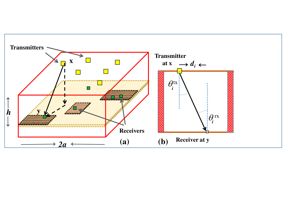
We consider an indoor downlink VLC network with optical attocells (OAs) operating at the same frequency band. We consider a room with height (desktop level to roof level) $h$ and length and width $2a$. Without loss of generality, we can assume that center of the room is at the origin. The 2D floor of the room is denoted by set $\mathcal{S}(0,a)$ where $\mathcal{S}({\mathbf{x}},a)$ denotes a square at center ${\mathbf{x}}$ with sides of length $2a$. The locations of OAs are modeled as a 2-D homogeneous Poisson point process (PPP) $\Phi=\{{\mathbf{x}}_{i}\in\mathbb{R}^{2}\}$ with a density of $\lambda$ on the roof top in area $\mathcal{S}(0,a)$. Hence, the $i\text{th}$ OA’s location is given as $({\mathbf{x}}_{i},h)$. Each OA consists of LEDs oriented vertically downwards. The users are distributed as a homogeneous PPP at the desktop level with density $\lambda_{\mathrm{u}}$ across the room. A typical user (i.e. arbitrarily selected user) is located uniformly in the room. Let us denote the location of the typical user with $({\mathbf{y}},0)$. Here, ${\mathbf{y}}=(y_{1},y_{2})\in\mathbb{R}^{2}$ such that $y_{1},y_{2}\sim\mathrm{U}(-a,a)$.

We assume that the transmitters follow Lambertian emission radiation profile and they operate within the linear dynamic range of the current-to-power characteristic curve. The channel direct current gain between the user and $i\text{th}$ OA can be modeled as follows [10]

$\displaystyle G_{i}=(m+1)\xi\frac{A_{pd}}{2\pi d_{i}^{2}}\cos^{m}(\theta_{i}^{\mathrm{tx}})\cos(\theta_{i}^{\mathrm{rx}})G_{\mathrm{c}}(\theta_{i}^{\mathrm{rx}})G_{\mathrm{f}}(\theta_{i}^{\mathrm{rx}})$

(1)

where $d_{i}$ is the distance of the user to $i\text{th}$ OA. $m$ denotes the order of Lambertian emission and is given as $m=1/{\log_{2}(\sec{\Psi_{\mathsf{HALF}}})}$ where $\Psi_{\mathsf{HALF}}$ is the semi angle of transmitter’s LEDs. $\theta_{i}^{\mathrm{tx}}$ and $\theta_{i}^{\mathrm{rx}}$ represent the $i\text{th}$ OA’s irradiance and incidence angle with respect to the user. $A_{pd}$ denotes the detection area of the photodetector (PD) at the receiver. $G_{\mathrm{f}}(\theta^{\mathrm{rx}}_{i})$ and $G_{\mathrm{c}}(\theta^{\mathrm{rx}}_{i})$ are the gains of the receiver’s optical filter and concentrator and assumed to be constant. $\xi$ denotes the average responsivity of PD. From Fig. 1(b), we can observe that

$\displaystyle\cos(\theta_{i}^{\mathrm{tx}})$

$\displaystyle=\cos(\theta_{i}^{\mathrm{rx}})={h}/{\sqrt{h^{2}+d_{i}^{2}}}.$

(2)

Substituting values of $\cos(\theta^{\mathrm{tx}}_{i})$ and $\cos(\theta^{\mathrm{rx}}_{i})$ into (1), we get

$\displaystyle G_{i}$

$\displaystyle=\alpha{(|{\mathbf{x}}_{i}-{\mathbf{y}}|^{2}+h^{2})}^{-\beta/2}$

where $\alpha=(m+1)A_{pd}\xi G_{\mathrm{f}}G_{\mathrm{c}}h^{m+1}/(2\pi)$ and $\beta=m+3$. The transmit power of OA is assumed to be $P_{\mathrm{tx}}$. We assume direct current OFDM as modulation scheme [10]. Hence, the receiver power from the $i\text{th}$ transmitter is given as

$\displaystyle P_{i}$

$\displaystyle=P_{\mathrm{tx}}\alpha^{2}\ell({\mathbf{x}},{\mathbf{y}}).$

(3)

where $\ell({\mathbf{x}},{\mathbf{y}})$ be defined as $\ell({\mathbf{x}},{\mathbf{y}})={(|{\mathbf{x}}-{\mathbf{y}}|^{2}+h^{2})}^{-\beta}$.

If the considered user is associated with $i\text{th}$ OA located at ${\mathbf{x}}_{i}$, the SINR at this user is given as

$\displaystyle\mathrm{SINR}_{i}({\mathbf{y}})$

$\displaystyle=\frac{\ell({\mathbf{x}}_{i},{\mathbf{y}})}{I(\Phi\setminus{\mathbf{x}}_{i})+\sigma^{2}}$

(4)

where $I$ denotes the sum interference and given as

$\displaystyle I(\Phi\setminus{\mathbf{x}}_{i})$

$\displaystyle=\sum_{{\mathbf{x}}_{j}\in\Phi\setminus{\mathbf{x}}_{i}}\ell({\mathbf{x}}_{j},{\mathbf{y}}).$

(5)

Here, $\sigma^{2}$ is effective noise and given as $\sigma^{2}=N_{0}B_{f}/(\alpha^{2}P_{\mathrm{tx}})$ with $N_{0}$ being the noise power spectral density and $B_{f}$ being the user bandwidth. We consider maximum received signal power-based association criterion which is equivalent to the nearest BS association criterion due to lack of random fading in the VLC environment. Suppose that the associated BS’s index is 0, then ${\mathbf{x}}_{0}=\arg\max_{{\mathbf{x}}_{i}}\ell({\mathbf{x}}_{i},{\mathbf{y}}).$ The SINR at this user is equal to $\mathrm{SINR}_{0}({\mathbf{y}})$. In the next sections, we will present analytical framework to compute performance of this typical user. We will first consider VLC networks without any reflections in the Section III. We then present a framework to model reflections in VLC network in the Section IV and extend the analysis to study their impact.

The SINR coverage probability $\mathrm{P}_{\mathrm{c}}(\tau,{\mathbf{y}})$ of a user located at ${\mathbf{y}}$ is defined as the probability that the SINR at this user is greater than the threshold $\tau$ i.e.

$\displaystyle\mathrm{P}_{\mathrm{c}}(\tau,{\mathbf{y}})=\mathbb{P}\left[\mathrm{SINR}_{0}({\mathbf{y}})>\tau\right].$

(6)

We assume that SINR threshold $\tau\geq 1$. From [12], it can be shown that at maximum, only one OA can have SINR greater than 1 (and hence $\tau$). In other words,

$\displaystyle\mathbbm{1}\left({\mathrm{SINR}_{0}({\mathbf{y}})>\tau}\right)$

$\displaystyle=\sum_{{\mathbf{x}}_{i}\in\Phi}\mathbbm{1}\left({\mathrm{SINR}_{i}({\mathbf{y}})>\tau}\right).$

Therefore, the probability of SINR coverage is given as

$\displaystyle\mathrm{P}_{\mathrm{c}}(\tau,{\mathbf{y}})$

$\displaystyle=\mathbb{E}\left[\sum_{{\mathbf{x}}_{i}\in\Phi}\mathbbm{1}\left({\mathrm{SINR}_{i}({\mathbf{y}})>\tau}\right)\right].$

(7)

From Campbell-Mecke theorem and Sliynak theorem [11], (7) can be further solved as

		$\displaystyle\mathrm{P}_{\mathrm{c}}(\tau,{\mathbf{y}})=\lambda\int_{\mathcal{S}(0,a)}\mathbb{P}\left[\frac{\ell({\mathbf{x}},{\mathbf{y}})}{I(\Phi)+\sigma^{2}}>\tau\right]\mathrm{d}{\mathbf{x}}$
		$\displaystyle=\lambda\int_{\mathcal{S}(0,a)}\mathbb{P}\left[I<\tau^{-1}{\left(|{\mathbf{x}}-{\mathbf{y}}|^{2}+h^{2}\right)}^{-\beta}-\sigma^{2}\right]\mathrm{d}{\mathbf{x}}$
		$\displaystyle=\lambda\int_{\mathcal{S}(-{\mathbf{y}},a)}\mathbb{P}\left[I<\tau^{-1}{\left(|{\mathbf{x}}|^{2}+h^{2}\right)}^{-\beta}-\sigma^{2}\right]\mathrm{d}{\mathbf{x}}.$		(8)

where the last step is due to the transformation ${\mathbf{x}}\rightarrow{\mathbf{x}}+{\mathbf{y}}$. Note that $\mathbb{P}\left[I<s\right]$ is non zero only when $s>0$ which is equivalent to $\{{\mathbf{x}}:|{\mathbf{x}}|<a_{\mathrm{D}}\stackrel{{\scriptstyle\Delta}}{{=}}\left[\tau^{-1/\beta}\sigma^{-2/\beta}-h^{2}\right]^{1/2}\}$. Now, (8) can be written as

$\displaystyle\mathrm{P}_{\mathrm{c}}(\tau,{\mathbf{y}})$

$\displaystyle=\lambda\int_{\mathsf{A}_{\mathbf{y}}}\mathbb{P}\left[I<\tau^{-1}{\left(|{\mathbf{x}}|^{2}+h^{2}\right)}^{-\beta}-\sigma^{2}\right]\mathrm{d}{\mathbf{x}}$

(9)

where $\mathsf{A}_{\mathbf{y}}=\mathcal{S}(-{\mathbf{y}},a)\cap\mathcal{B}(0,a_{\mathrm{D}})$. Here, $\mathcal{B}(\mathbf{a},r)$ denotes a ball of radius $r$ and center $\mathbf{a}$. Note that due to absence of fading, there is a certain radius $a_{\mathrm{D}}$ around the receiver in which associated OA must be located otherwise the signal strength is smaller than the noise power, making SNR (and hence SINR) less that $\tau$. From the Gill Pelaez inversion Lemma [13], the CDF of the sum interference $I$ can be expressed in terms of its Laplace transform $\mathcal{L}_{I}()$ as

$\displaystyle\mathbb{P}\left[I<s\right]$

$\displaystyle=\frac{1}{2}-\frac{1}{\pi}\int_{0}^{\infty}\frac{1}{t}\mathrm{Im}\left[e^{-jts}\mathcal{L}_{I}(-jt)\right]\mathrm{d}t.$

(10)

From (9) and (10), the SINR coverage probability is

$\displaystyle\mathrm{P}_{\mathrm{c}}(\tau,{\mathbf{y}})=$

$\displaystyle\lambda\int_{\mathsf{A}({\mathbf{y}})}\left[\frac{1}{2}-\frac{1}{\pi}\int_{0}^{\infty}\frac{1}{t}\mathrm{Im}\left[e^{-jt(\tau^{-1}{\left(|{\mathbf{x}}|^{2}+h^{2}\right)}^{-\beta}-\sigma^{2})}\right.\right.\left.\left.\vphantom{\frac{3}{4}}\mathcal{L}_{I}\left(-jt\right)\right]\mathrm{d}t\right]\mathrm{d}{\mathbf{x}}.$

(11)

Note that (11) requires computation of $\mathcal{L}_{I}()$ which we give in the following Lemma.

In this section, we derive the rate coverage which is defined as the probability that the rate of a user at ${\mathbf{y}}$ is greater than the threshold $\rho$,

$\displaystyle\mathrm{R}_{\mathrm{c}}(\rho,{\mathbf{y}})=\mathbb{P}\left[\mathrm{Rate}_{0}({\mathbf{y}})>\rho\right].$

(15)

Let $W$ be the total bandwidth available at each OA. Assuming the time-division access for providing access to mutiple users at a single OA [8], the per user rate can be given as [9]

$\displaystyle\mathrm{Rate}$

$\displaystyle=\zeta_{1}\frac{W}{n}\log{\left(1+\zeta_{2}\mathrm{SINR}\right)}.$

(16)

where $n$ is the mean number of users (or load) associated with the serving OA and $\zeta_{1},\zeta_{2}$ are some coefficients due to practical constraints. Since the user distribution is also assumed to be PPP, the mean load with the typical user can be modeled similarly to [14] to be $n=1+1.28\lambda_{\mathrm{u}}/\lambda$. Now, $\mathrm{R}_{\mathrm{c}(}\rho,{\mathbf{y}})$ can be derived in terms of coverage probability as follows:

		$\displaystyle\mathrm{R}_{\mathrm{c}}(\rho,{\mathbf{y}})=\mathbb{P}\left[\mathrm{Rate}({\mathbf{y}})>\rho\right]$
		$\displaystyle=\mathbb{P}\left[\frac{W\zeta_{1}}{n}\log{(1+\zeta_{2}\mathrm{SINR}({\mathbf{y}}))}>\rho\right]$
		$\displaystyle=\mathbb{P}\left[\mathrm{SINR}>{\scriptstyle{\zeta_{2}^{-1}}}(2^{\rho\frac{n}{W\zeta_{1}}}-1)\right]=\mathrm{P}_{\mathrm{c}}\left({\scriptstyle\zeta_{2}^{-1}}(2^{\rho n/(W\zeta_{1})}-1),{\mathbf{y}}\right)$

where $\mathrm{P}_{\mathrm{c}}$ is given in (13). The rate coverage for an arbitrarily located typical user is given as

$\displaystyle\mathrm{R}_{\mathrm{c}}(\rho)$

$\displaystyle=\mathrm{P}_{\mathrm{c}}\left(\zeta_{2}\left(2^{\zeta_{1}^{-1}\rho n/W}-1\right)\right).$

(17)

Reflections can be modeled using image of the original transmitters with respect to the walls (See Fig. 2(a))[15]. Let us first consider single reflections. For a given Tx-Rx pair, there are total 4 reflection images formed on the other side of walls (See Fig. 2(b)). The first reflection images of transmitters (let us call them virtual transmitters) form a PPP $\Phi_{1}$ with density $\lambda$ in the area $\mathsf{F}_{\mathrm{I}}=\mathcal{S}(0,a)\oplus 2a\mathsf{G}_{1}$ (See vertically shaded area in Fig. 2(c)) where $\mathsf{G}_{1}=\{(\pm 1,0),(0,\pm 1)\}$ and $\oplus$ denotes the Minkowski sum of two sets. The received power at the user ${\mathbf{y}}$ from a virtual transmitter located at ${\mathbf{x}}$ is given as (See Fig. 2(a))

$\displaystyle\ell({\mathbf{x}},{\mathbf{y}})=\eta{(|{\mathbf{x}}-{\mathbf{y}}|^{2}+h^{2})}^{-\beta},\ {\mathbf{x}}\in\mathsf{F}_{\mathrm{I}}$

(18)

where $\eta$ is due to reflection loss and dependent on the wall material [16]. Combining the path-loss for ${\mathbf{x}}\in\mathcal{S}(0,a)$ (given in (3) and ${\mathbf{x}}\in\mathsf{F}_{\mathrm{I}}$ (given in (18)), we get the following pathloss function

$\displaystyle\ell({\mathbf{x}},{\mathbf{y}})$

$\displaystyle=\begin{cases}{(|{\mathbf{x}}-{\mathbf{y}}|^{2}+h^{2})}^{-\beta},&{\mathbf{x}}\in\mathcal{S}(0,a)\\ \eta{(|{\mathbf{x}}-{\mathbf{y}}|^{2}+h^{2})}^{-\beta},&{\mathbf{x}}\in\mathsf{F}_{\mathrm{I}}\end{cases}.$

Similarly second reflection images of transmitters (also virtual transmitters) form a PPP $\Phi_{2}$ with density $\lambda$ in the area $\mathsf{F}_{\mathrm{II}}=\mathcal{S}(0,a)\oplus 4a\mathsf{G}_{2}$ (See horizontally shaded area in Fig. 2(c)) where $\mathsf{G}_{2}=\left\{(0,\pm 1),(\pm 1,0),\left(\pm\frac{1}{2},\pm\frac{1}{2}\right)\right\}$ with reflection loss coefficient $\eta^{2}$. In general, $k\text{th}$ reflection images of transmitters form a PPP $\Phi_{k}$ in the area $\mathsf{F}_{\mathrm{k}}=\mathcal{S}(0,a)\oplus 2ka\mathsf{G}_{k}$ with reflection loss coefficient as $\eta^{k}$ where $\mathsf{G}_{k}=\left\{\left(\pm\frac{k_{1}}{k},\pm\frac{k_{2}}{k}\right):k_{1}+k_{2}=k,k_{1}\in\mathbb{N}\right\}$. Note that the cardinality of $\mathsf{G}_{k}$ is $|\mathsf{G}_{k}|=4k$ (for $k>0$). Let us define $\mathsf{G}_{0}=\{(0,0)\}$ and $\mathsf{F}_{0}=\mathcal{S}(0,a)$ for completeness. Hence, the aggregate pathloss function considering all transmitters (real and virtual) is given as

$\displaystyle\ell({\mathbf{x}},{\mathbf{y}})$

$\displaystyle=\begin{cases}{(|{\mathbf{x}}-{\mathbf{y}}|^{2}+h^{2})}^{-\beta},&\text{if }{\mathbf{x}}\in\mathcal{S}(0,a)\\ \eta^{k}{(|{\mathbf{x}}-{\mathbf{y}}|^{2}+h^{2})}^{-\beta},&\parbox{144.54pt}{if ${\mathbf{x}}\in\mathcal{S}(0,a)$ $\oplus 2ak\mathsf{G}_{k}$.}\end{cases}$

(19)

Note that all sets $\mathsf{F}_{\mathrm{k}}$ are mutually disjoint and cover whole space $\mathbb{R}^{2}$. We have assumed their independence. Therefore, the union of all reflection images and real transmitters form a PPP with density $\lambda$ due to the superposition theorem [12].

Let us consider reflections upto the $K\text{th}$ order only. In this case, the union of all transmitters will be a PPP over the space $\cup_{k}\mathsf{F}_{\mathrm{k}}$. Now, similar to the no reflection case, we can apply Campbell-Mecke theorem and Sliynak theorem in (7) to get

		$\displaystyle\mathrm{P}_{\mathrm{c}}(\tau,{\mathbf{y}})=\lambda\sum_{k=0}^{K}\int_{\mathsf{F}_{\mathrm{k}}(0,a)}\mathbb{P}\left[\frac{\ell({\mathbf{x}},{\mathbf{y}})}{I(\Phi)+\sigma^{2}}>\tau\right]\mathrm{d}{\mathbf{x}}$
		$\displaystyle=\lambda\sum_{k=0}^{K}\int_{\mathsf{F}_{\mathrm{k}}(0,a)}\mathbb{P}\left[I<\tau^{-1}{\eta^{k}\left(|{\mathbf{x}}-{\mathbf{y}}|^{2}+h^{2}\right)}^{-\beta}-\sigma^{2}\right]\mathrm{d}{\mathbf{x}}$
		$\displaystyle=\lambda\sum_{k=0}^{K}\int_{\mathsf{F}_{\mathrm{k}}(-{\mathbf{y}},a)}\mathbb{P}\left[I<\tau^{-1}\eta^{k}{\left(|{\mathbf{x}}|^{2}+h^{2}\right)}^{-\beta}-\sigma^{2}\right]\mathrm{d}{\mathbf{x}}$		(20)

where $\mathsf{F}_{\mathrm{k}}(-{\mathbf{y}},a)$ is the translation of the set $\mathsf{F}_{\mathrm{k}}(0,a)$ by the vector ${\mathbf{y}}$. Note that $\mathbb{P}\left[I<\cdot\right]$ is non-zero only for $\{{\mathbf{x}}:|{\mathbf{x}}|<b^{k}_{\mathrm{D}}\stackrel{{\scriptstyle\Delta}}{{=}}\left[\eta^{k/\beta}{(\tau\sigma^{2})}^{-1/\beta}-h^{2}\right]^{1/2}\}$. Hence, (20) is written as

$\displaystyle\mathrm{P}_{\mathrm{c}}(\tau,{\mathbf{y}})$

$\displaystyle=\lambda\sum_{k=0}^{K}\int_{\mathsf{B}_{k{\mathbf{y}}}}\mathbb{P}\left[I<\eta^{k}\tau^{-1}{\left(|{\mathbf{x}}|^{2}+h^{2}\right)}^{-\beta}-\sigma^{2}\right]\mathrm{d}{\mathbf{x}}$

where $\mathsf{B}_{k{\mathbf{y}}}=\mathsf{F}_{\mathrm{k}}(-{\mathbf{y}},a)\cap\mathcal{B}\left(0,b^{k}_{\mathrm{D}}\right)$. Here, $b^{k}_{\mathrm{D}}$ shows the radius in which virtual transmitter of $k\text{th}$ order must be located. Now, following the steps similar to Appendix A, we can compute the Laplace transform of interference which is given in the following Lemma.

Using Lemma 1 and the Gil-Paleaz Lemma similar to the previous section, we get the following theorem.

References

- [1] L. Feng, R. Q. Hu, J. Wang, P. Xu, and Y. Qian, “Applying VLC in 5G networks: Architectures and key technologies,” IEEE Network, vol. 30, no. 6, pp. 77–83, Nov. 2016.
- [2] A. Jovicic, J. Li, and T. Richardson, “Visible light communication: opportunities, challenges and the path to market,” IEEE Commun. Mag., vol. 51, no. 12, pp. 26–32, Dec. 2013.
- [3] D. Karunatilaka, F. Zafar, V. Kalavally, and R. Parthiban, “LED based indoor visible light communications: state of the art,” IEEE Commun. Surveys & Tut., vol. 17, no. 3, pp. 1649–1678, 2015.
- [4] H. Elgala, R. Mesleh, and H. Haas, “Indoor optical wireless communication: Potential and state-of-the-art,” IEEE Commun. Mag., vol. 49, no. 9, pp. 56–62, Sep. 2011.
- [5] P. H. Pathak, X. Feng, P. Hu, and P. Mohapatra, “Visible light communication, networking, and sensing: A survey, potential and challenges,” IEEE Commun. Surveys Tut., vol. 17, no. 4, pp. 2047–2077, Fourthquarter 2015.
- [6] A. Vavoulas, H. G. Sandalidis, T. A. Tsiftsis, and N. Vaiopoulos, “Coverage aspects of indoor VLC networks,” Journal of Lightwave Technology, vol. 33, no. 23, pp. 4915–4921, 2015.
- [7] T. Komine and M. Nakagawa, “Fundamental analysis for visible light communication system using LED lights,” IEEE Trans. Consumer Electronics, vol. 50, no. 1, pp. 100–107, Feb. 2004.
- [8] C. Chen, D. A. Basnayaka, and H. Haas, “Downlink performance of optical attocell networks,” Journal of Lightwave Technology, vol. 34, no. 1, pp. 137–156, Jan 2016.
- [9] H. Tabassum and E. Hossain, “Coverage and rate analysis for co-existing RF/VLC downlink cellular networks,” ArXiv:preprint:1710.01272, Oct 2017.
- [10] L. Yin and H. Haas, “Coverage analysis of multiuser visible light communication networks,” IEEE Trans. Wireless Commun., vol. PP, no. 99, pp. 1–1, 2017.
- [11] F. Baccelli and B. Błaszczyszyn, Stochastic Geometry and Wireless Networks, 2nd ed. NOW Publishers, 2009, vol. 1.
- [12] J. G. Andrews, A. K. Gupta, and H. S. Dhillon, “A primer on cellular network analysis using stochastic geometry,” arXiv preprint arXiv:1604.03183, 2016.
- [13] J. Gil-Pelaez, “Note on the inversion theorem,” Biometrika, vol. 38, no. 3-4, pp. 481–482, 1951.
- [14] S. Singh, H. S. Dhillon, and J. G. Andrews, “Offloading in heterogeneous networks: modeling, analysis and design insights,” IEEE Trans. Wireless Commun., vol. 12, no. 5, pp. 2484 – 2497, May 2013.
- [15] K. Venugopal and R. W. Heath, “Millimeter wave networked wearables in dense indoor environments,” IEEE Access, vol. 4, pp. 1205–1221, 2016.
- [16] W. J. Smith, Modern Optical Engineering, 4th ed. McGraw Hill Education, 2007.