跳到论文正文
W Papers独立论文阅读器 arXiv:1804.04385 论文正文 计算阅读时间 · 0%
引用这篇论文根据当前论文元数据生成,正式投稿前建议核对。


License: arXiv.org perpetual non-exclusive license
arXiv:1804.04385v3 [math.NA] 10 Apr 2020

Convergence of a Finite Volume Scheme for a System of Interacting Species with Cross-Diffusion

Abstract.

In this work we present the convergence of a positivity preserving semi-discrete finite volume scheme for a coupled system of two non-local partial differential equations with cross-diffusion. The key to proving the convergence result is to establish positivity in order to obtain a discrete energy estimate to obtain compactness. We numerically observe the convergence to reference solutions with a first order accuracy in space. Moreover we recover segregated stationary states in spite of the regularising effect of the self-diffusion. However, if the self-diffusion or the cross-diffusion is strong enough, mixing occurs while both densities remain continuous.

Key words and phrases: 
Finite volume methods; Integro-partial differential equations; Population dynamics (general); Developmental biology, pattern formation;
2010 Mathematics Subject Classification
Primary: 74S10; 65M12; 92C15; Secondary: 45K05; 92D25; 47N60

José A. Carrillo

Mathematical Institute, University of Oxford

Oxford OX2 6GG, United Kingdom

Francis Filbet

Institut de Mathématiques de Toulouse, Université Paul Sabatier

Toulouse, France

Markus Schmidtchen

Laboratoire Jacques-Louis Lions, Sorbonne Université

4 place Jussieu, 75005 Paris, France

1. Introduction

In this paper we develop and analyse a numerical scheme for the following non-local interaction system with cross-diffusion and self-diffusion

{∂ρ∂t=∂∂x​(ρ​∂∂x​(W11⋆ρ+W12⋆η+ν⁡(ρ+η))+ϵ2​∂ρ2∂x),∂η∂t=∂∂x​(η​∂∂x​(W22⋆η+W21⋆ρ+ν⁡(ρ+η))+ϵ2​∂η2∂x),\displaystyle\left\{\begin{array}[]{r}\displaystyle\frac{\partial\rho}{\partial t}=\displaystyle\frac{\partial}{\partial x}\left(\rho\frac{\partial}{\partial x}\left(W_{11}\star\rho+W_{12}\star\eta+\nu(\rho+\eta)\right)\,+\,\dfrac{\epsilon}{2}\frac{\partial\rho^{2}}{\partial x}\right),\\[17.50002pt] \displaystyle\frac{\partial\eta}{\partial t}=\displaystyle\frac{\partial}{\partial x}\left(\eta\frac{\partial}{\partial x}\left(W_{22}\star\eta+W_{21}\star\rho+\nu(\rho+\eta)\right)\,+\,\dfrac{\epsilon}{2}\frac{\partial\eta^{2}}{\partial x}\right),\end{array}\right.

governing the evolution of two species ρ\rho and η\eta on an interval (a,b)⊂ℝ(a,b)\subset\mathbb{R} for t∈[0,T)t\in[0,T). The system is equipped with nonnegative initial data ρ0,η0∈L+1​(a,b)∩L+∞​(a,b)\rho^{0},\eta^{0}\in L_{+}^{1}(a,b)\cap L_{+}^{\infty}(a,b). We denote by m1m_{1} the mass of ρ0\rho_{0} and by m2m_{2} the mass of η0\eta_{0}, respectively,

m1=∫abρ0​(x)​𝑑x,andm2=∫abη0​(x)​𝑑x.m_{1}\,=\,\int_{a}^{b}\rho_{0}(x)\,{\rm{d}}x,\quad\text{and}\quad m_{2}\,=\,\int_{a}^{b}\eta_{0}(x)\,{\rm{d}}x.

On the boundary x=ax=a and bb, we prescribe no-flux boundary conditions

{ρ​∂∂x​(W11⋆ρ+W12⋆η+ν⁡(ρ+η)+ϵ​ρ)=0,η​∂∂x​(W22⋆η+W21⋆ρ+ν⁡(ρ+η)+ϵ​η)=0,\displaystyle\left\{\begin{array}[]{r}\displaystyle\rho\,\frac{\partial}{\partial x}\left(W_{11}\star\rho+W_{12}\star\eta+\nu(\rho+\eta)+\epsilon\rho\right)=0,\\ \\ \displaystyle\eta\,\frac{\partial}{\partial x}\left(W_{22}\star\eta+W_{21}\star\rho+\nu(\rho+\eta)+\epsilon\eta\right)=0,\end{array}\right.

such that the total mass of each species is conserved with respect to time t≥0t\geq 0. While the self-interaction potentials W11,W22∈Cb2​(ℝ)W_{11},W_{22}\in C_{b}^{2}(\mathbb{R}) model the interactions among individuals of the same species (also referred to as intraspecific interactions), the cross-interaction potentials W12,W21∈Cb2​(ℝ)W_{12},W_{21}\in C_{b}^{2}(\mathbb{R}) encode the interactions between individuals belonging to different species, i.e. interspecific interactions. Here Cb2​(ℝ)C_{b}^{2}(\mathbb{R}) denotes the set of twice continuously differentiable functions on ℝ\mathbb{R} with bounded derivatives. Notice that the convolutions Wi​j⋆ψW_{ij}\star\psi, with ψ\psi a density function defined on [a,b][a,b], are defined by extending the density ψ\psi by zero outside the interval [a,b][a,b]. The two positive parameters ϵ,ν>0\epsilon,\nu>0 determine the strengths of the self-diffusion and the cross-diffusion of both species, respectively. Nonlinear diffusion, be it self-diffusion or cross-diffusion, is biologically relevant. As a matter of fact, around the second half of the 20th20^{\mathrm{th}} century biologists found that the dispersal rate of certain insects depends on the density itself, leading to the nonlinear diffusion terms we incorporated in the model, cf. [36, 37, 34, 13, 32]. At the same time we would like to stress that the self-diffusion terms are relevant for the convergence analysis below.

It is the interplay between the non-local interactions of both species and their individual and joint size-exclusion, modelled by the non-linear diffusion [5, 4, 6, 40, 12, 10], that leads to a large variety of behaviours including complete phase separation or mixing of both densities in both stationary configurations and travelling pulses [11, 19].

While their single species counterparts have been studied quite intensively [35, 21, 41, 15] and references therein, related two-species models like the system of our interest, Eq. (1), have only recently gained considerable attention [25, 11, 19, 24, 17]. One of the most striking phenomena of these interaction models with cross-diffusion is the possibility of phase separation. Since the seminal papers [33, 5] established segregation effects for the first time for the purely diffusive system corresponding to (1) for Wi​j≡0W_{ij}\equiv 0, i,j∈{1,2}i,j\in\{1,2\} and ϵ=0\epsilon=0, many generalisations were presented. This includes reaction-(cross-)diffusion systems [3, 7, 17] and references therein, and by adding non-local interactions [11, 19, 24, 2] and references therein. Ref. [24] have established the existence of weak solutions to a class of non-local systems under a strong coercivity assumption on the cross-diffusion also satisfied by system (1).

Typical applications of these non-local models comprise many biological contexts such cell-cell adhesion [39, 38, 16], for instance, as well as tumour models [31, 26], but also the formation of the characteristic stripe patterns of zebrafish can be modelled by these non-local models [42]. Systems of this kind are truly ubiquitous in nature and we remark that ‘species’ may not only refer to biological species but also to a much wider class of (possibly inanimate) agents such as planets, physical or chemical particles, just to name a few.

Since system (1) is in conservative form a finite volume scheme is a natural choice as a numerical method. This is owing to the fact that, by construction, finite volume schemes are locally conservative: due to the divergence theorem, the change in density on a test cell has to equal the sum of the in-flux and the out-flux of the same cell. There is a huge literature on finite volume schemes, first and foremost [28]. Therein, the authors give a detailed description of the construction of such methods and address convergence issues. Schemes similar to the one proposed in Section 2 have been studied in [9] in the case of nonlinear degenerate diffusion equations in any dimension. A similar scheme for a system of two coupled PDEs was proposed in [22]. Later, the authors in [14] generalised the scheme proposed in [9] including both local and non-local drifts. The scheme was then extended to two species in [19]. All the aforementioned schemes have in common that they preserve nonnegativity – a property that is also crucial for our analysis.

Before we define the finite volume scheme we shall present a formal energy estimate for the continuous system. The main difficulty in this paper is to establish positivity and reproducing the continuous energy estimate at the discrete level. The remainder of the introduction is dedicated to presenting the aforementioned energy estimate. Let us consider

dd​t​∫abρ​log⁡ρ​𝑑x\displaystyle\displaystyle\frac{{\rm{d}}}{{\rm{d}}t}\int_{a}^{b}\rho\log\rho\,{\rm{d}}x =∫ablog⁡ρ​∂ρ∂t​𝑑x\displaystyle=\displaystyle\int_{a}^{b}\log\rho\,\frac{\partial\rho}{\partial t}\,{\rm{d}}x
=∫ablog⁡ρ​∂∂x​(ρ​∂∂x​(W11⋆ρ+W12⋆η+ν⁡(ρ+η)+ϵ​ρ))​𝑑x\displaystyle=\displaystyle\int_{a}^{b}\log\rho\,\frac{\partial}{\partial x}\left(\rho\frac{\partial}{\partial x}\left(W_{11}\star\rho+W_{12}\star\eta+\nu(\rho+\eta)+\epsilon\rho\right)\right){\rm{d}}x
=−∫abρ∂∂x(W11⋆ρ+W12⋆η+ν(ρ+η)+ϵρ)∂∂x(logρ)dx,\displaystyle=\displaystyle-\int_{a}^{b}\rho\,\frac{\partial}{\partial x}\left(W_{11}\star\rho+W_{12}\star\eta+\nu(\rho+\eta)+\epsilon\rho\right)\,\frac{\partial}{\partial x}(\log\rho)\,{\rm{d}}x,

where the second equality holds due to the no-flux boundary conditions. Upon rearranging we get

dd​t∫abρlogρdx+ν∫ab∂∂x(ρ+η)∂ρ∂xdx+ϵ∫ab|∂ρ∂x|2dx=−∫ab(W11′⋆ρ+W12′⋆η)∂ρ∂xdx.\displaystyle\frac{{\rm{d}}}{{\rm{d}}t}\int_{a}^{b}\rho\log\rho\,{\rm{d}}x\,+\,\nu\,\int_{a}^{b}\frac{\partial}{\partial x}(\rho+\eta)\frac{\partial\rho}{\partial x}\,{\rm{d}}x\,+\,\epsilon\int_{a}^{b}\left|\frac{\partial\rho}{\partial x}\right|^{2}\,{\rm{d}}x\,=\,-\int_{a}^{b}(W_{11}^{\prime}\star\rho+W_{12}^{\prime}\star\eta)\,\frac{\partial\rho}{\partial x}\,{\rm{d}}x.

A similar computation for η\eta yields

dd​t∫abηlogηdx+ν∫ab∂∂x(ρ+η)∂η∂xdx+ϵ∫ab|∂η∂x|2dx=−∫ab(W22′⋆η+W21′⋆ρ)∂η∂xdx,\displaystyle\frac{{\rm{d}}}{{\rm{d}}t}\int_{a}^{b}\eta\log\eta\,{\rm{d}}x\,+\,\nu\,\int_{a}^{b}\frac{\partial}{\partial x}(\rho+\eta)\,\frac{\partial\eta}{\partial x}\,{\rm{d}}x\,+\,\epsilon\,\int_{a}^{b}\left|\frac{\partial\eta}{\partial x}\right|^{2}\,{\rm{d}}x\,=\,-\int_{a}^{b}(W_{22}^{\prime}\star\eta+W_{21}^{\prime}\star\rho)\,\frac{\partial\eta}{\partial x}\,{\rm{d}}x,

whence, upon adding both, we obtain

dd​t​∫ab[ρ​log⁡ρ+η​log⁡η]​dx+ν​∫ab|∂σ∂x|2​dx+ϵ​∫ab(|∂ρ∂x|2+|∂η∂x|2)​dx=𝒟ρ+𝒟η,\begin{array}[]{rcl}\displaystyle\frac{{\rm{d}}}{{\rm{d}}t}\int_{a}^{b}\left[\rho\log\rho+\eta\log\eta\right]\,{\rm{d}}x\,+\,\displaystyle\nu\int_{a}^{b}\left|\frac{\partial\sigma}{\partial x}\right|^{2}{\rm{d}}x\,+\,\epsilon\,\int_{a}^{b}\left(\left|\frac{\partial\rho}{\partial x}\right|^{2}\,+\,\left|\frac{\partial\eta}{\partial x}\right|^{2}\right)\,{\rm{d}}x\,=\,\displaystyle\mathcal{D}_{\rho}+\mathcal{D}_{\eta},\end{array}

where σ=ρ+η\sigma=\rho+\eta and

{𝒟ρ:=−∫ab(W11′⋆ρ+W12′⋆η)∂ρ∂xdx,𝒟η:=−∫ab(W22′⋆η+W21′⋆ρ)∂η∂xdx,\left\{\begin{array}[]{l}\mathcal{D}_{\rho}:=-\displaystyle\int_{a}^{b}(W_{11}^{\prime}\star\rho+W_{12}^{\prime}\star\eta)\,\frac{\partial\rho}{\partial x}\,{\rm{d}}x,\\[10.00002pt] \mathcal{D}_{\eta}:=-\displaystyle\int_{a}^{b}(W_{22}^{\prime}\star\eta+W_{21}^{\prime}\star\rho)\,\frac{\partial\eta}{\partial x}\,{\rm{d}}x,\end{array}\right.

denote the advective parts associated to ρ\rho and η\eta, respectively. The advective parts can be controlled by using the weighted Young inequality to get

|𝒟ρ|\displaystyle\displaystyle|\mathcal{D}_{\rho}| =|∫ab(W11′⋆ρ+W12′⋆η)​∂ρ∂x​𝑑x|\displaystyle=\displaystyle\left|\int_{a}^{b}(W_{11}^{\prime}\star\rho+W_{12}^{\prime}\star\eta)\frac{\partial\rho}{\partial x}\,{\rm{d}}x\right|
≤12​α​∫ab|W11′⋆ρ+W12′⋆η|2​𝑑x+α2​∫ab|∂ρ∂x|2​𝑑x,\displaystyle\leq\displaystyle\frac{1}{2\alpha}\int_{a}^{b}{|W_{11}^{\prime}\star\rho+W_{12}^{\prime}\star\eta|^{2}}\,{\rm{d}}x\,+\,\frac{\alpha}{2}\int_{a}^{b}\left|\frac{\partial\rho}{\partial x}\right|^{2}\,{\rm{d}}x,

for some α>0\alpha>0. In choosing 0<α<ϵ0<\alpha<\epsilon we obtain

(3) dd​t​∫ab[ρ​log⁡ρ+η​log⁡η]​𝑑x+ν​∫ab|∂σ∂x|2​𝑑x+(ϵ−α2)​∫ab(|∂ρ∂x|2+|∂η∂x|2)​𝑑x≤Cρ+Cη2​α,\displaystyle\frac{{\rm{d}}}{{\rm{d}}t}\int_{a}^{b}\left[\rho\log\rho+\eta\log\eta\right]\,{\rm{d}}x\,+\,\nu\int_{a}^{b}\left|\frac{\partial\sigma}{\partial x}\right|^{2}\,{\rm{d}}x\,+\,\left(\epsilon-\frac{\alpha}{2}\right)\,\int_{a}^{b}\left(\left|\frac{\partial\rho}{\partial x}\right|^{2}\,+\,\left|\frac{\partial\eta}{\partial x}\right|^{2}\right)\,{\rm{d}}x\,\leq\,\frac{C_{\rho}+C_{\eta}}{2\alpha},

where Cρ=‖W11′⋆ρ+W12′⋆η‖L22C_{\rho}=\|W_{11}^{\prime}\star\rho+W_{12}^{\prime}\star\eta\|_{L^{2}}^{2} and Cη=‖W22′⋆η+W21′⋆ρ‖L22C_{\eta}=\|W_{22}^{\prime}\star\eta+W_{21}^{\prime}\star\rho\|_{L^{2}}^{2}. From the last line, Eq. (3), we may deduce bounds on the gradient of each species as well as on their sum. As mentioned above the crucial ingredient for this estimate is the positivity of solutions.

The rest of this paper is organised as follows. In the subsequent section we present a semi-discrete finite volume approximation of system (1) and we present the main result, Theorem 2.4. Section 3 is dedicated to establishing positivity and to the derivation of a priori estimates. In Section 4 we obtain compactness, pass to the limit, and identify the limiting functions as weak solutions to system (1). We conclude the paper with a numerical exploration in Section 6. We study the numerical order of accuracy and discuss stationary states and phase segregation phenomena.

2. Numerical scheme and main result

In this section we introduce the semi-discrete finite volume scheme for system (1). To begin with, let us introduce our notion of weak solutions.

Definition 2.1 (Weak solutions.).

A couple of functions (ρ,η)(\rho,\eta) ∈\in L2​(0,T,H1​(a,b))2L^{2}(0,T;H^{1}(a,b))^{2} is a weak solution to system (1) if it satisfies

(4a) −∫abρ0φ(0,⋅)dx=∫0T∫ab[ρ(∂φ∂t+(−ν∂σ∂x+∂V1∂x)∂φ∂x)+ϵ2ρ2∂2φ∂x2]dxdt,\displaystyle\begin{split}-\int_{a}^{b}\rho_{0}\,\varphi(0,\cdot)\,{\rm{d}}x\,=\!\int_{0}^{T}\int_{a}^{b}\left[\rho\,\left(\frac{\partial\varphi}{\partial t}\,+\,\left(-\nu\frac{\partial\sigma}{\partial x}\,+\,\frac{\partial V_{1}}{\partial x}\right)\,\frac{\partial\varphi}{\partial x}\right)\,+\,\frac{\epsilon}{2}\,\rho^{2}\,\frac{\partial^{2}\varphi}{\partial x^{2}}\right]\,{\rm{d}}x\,{\rm{d}}t,\end{split}
and
(4b) −∫abη0φ(0,⋅)dx=∫0T∫ab[η(∂φ∂t+(−ν∂σ∂x+∂V2∂x)∂φ∂x)+ϵ2η2∂2φ∂x2]dxdt,\displaystyle\begin{split}-\int_{a}^{b}\eta_{0}\,\varphi(0,\cdot)\,{\rm{d}}x\,=\,\!\int_{0}^{T}\int_{a}^{b}\left[\eta\left(\frac{\partial\varphi}{\partial t}+\left(-\nu\frac{\partial\sigma}{\partial x}\,+\,\frac{\partial V_{2}}{\partial x}\right)\,\frac{\partial\varphi}{\partial x}\right)\,+\,\frac{\epsilon}{2}\,\eta^{2}\,\frac{\partial^{2}\varphi}{\partial x^{2}}\right]\,{\rm{d}}x{\rm{d}}t,\end{split}

respectively, for any φ∈Cc∞​([0,T)×(a,b),ℝ)\varphi\in C_{c}^{\infty}([0,T)\times(a,b);\mathbb{R}). Here we have set Vk=−Wk​ 1⋆ρ−Wk​ 2⋆ηV_{k}=-W_{k\,1}\star\rho-W_{k\,2}\star\eta, for k∈{1,2}k\in\{1,2\}, and σ=ρ+η\sigma=\rho+\eta, as above.

Notice that the existence of weak solutions to system (1) will follow directly from the convergence of the numerical solution. Indeed, our analysis relies on a compactness argument which does not suppose a priori existence of solution to system (1).

To this end we first define the following space discretisation of the domain.

Definition 2.2 (Space discretisation).

To discretise space, we introduce the mesh

𝒯:=⋃i∈ICi,\displaystyle\mathcal{T}:=\bigcup_{i\in I}C_{i},

where the control volumes are given by Ci=[xi−1/2,xi+1/2)C_{i}=[x_{i-1/2},x_{i+1/2}) for all i∈I:={1,…,N}i\in I:=\{1,\ldots,N\}. We assume that the measure of the control volumes are given by |Ci|=Δ​xi=xi+1/2−xi−1/2>0|C_{i}|=\Delta x_{i}=x_{i+1/2}-x_{i-1/2}>0, for all i∈Ii\in I. Note that x1/2=ax_{1/2}=a, and xN+1/2=bx_{N+1/2}=b.

xi−3/2x_{i-3/2}xi−1/2x_{i-1/2}xi+1/2x_{i+1/2}xi+3/2x_{i+3/2}xi−1x_{i-1}xix_{i}xi+1x_{i+1}CiC_{i}Ci−1C_{i-1}Ci+1C_{i+1}x1/2=ax_{1/2}=axN+1/2=bx_{N+1/2}=b
Figure 1. Space discretisation according to Definition 2.2.

We also define xi=(xi+1/2+xi−1/2)/2x_{i}=(x_{i+1/2}+x_{i-1/2})/2 the centre of cell CiC_{i} and set Δ​xi+1/2=xi+1−xi\Delta x_{i+1/2}=x_{i+1}-x_{i} for i=1,…,N−1i=1,\ldots,N-1. We assume that the mesh is regular in the sense that there exists ξ∈(0,1)\xi\in(0,1) such that for h:=max1≤i≤N⁡{Δ​xi}h:=\max_{1\leq i\leq N}\{\Delta x_{i}\}

(5) ξ​h≤Δ​xi≤h,\xi\,h\,\leq\,\Delta x_{i}\,\leq\,h,

and, as a consequence, ξ​h≤Δ​xi+1/2≤h\xi\,h\,\leq\,\Delta x_{{i+1/2}}\,\leq\,h, as well.

On this mesh we shall now define the semi-discrete finite volume approximation of system (1). The discretised initial data are given by the cell averages of the continuous initial data, i.e.

(6) ρi0:=1Δ​xi​∫Ciρ0​(x)​𝑑x,andηi0:=1Δ​xi​∫Ciη0​(x)​𝑑x,\displaystyle\rho_{i}^{0}:=\frac{1}{\Delta x_{i}}\int_{C_{i}}\rho_{0}(x)\,{\rm{d}}x,\qquad\text{and}\qquad\eta_{i}^{0}:=\frac{1}{\Delta x_{i}}\int_{C_{i}}\eta_{0}(x)\,{\rm{d}}x,

for all i∈Ii\in I. Throughout, we write ρi\rho_{i} (resp. ηi\eta_{i}) to denote the approximations of the two densities on the ii-th finite volume cell, CiC_{i}. Next, we introduce the discrete versions of the cross-diffusion and the interaction terms. We set

{(V1)i:=−∑j=1NΔxj(W11i−jρj+W12i−jηj),(V2)i:=−∑j=1NΔxj(W22i−jηj+W21i−jρj),\displaystyle\left\{\begin{array}[]{ll}\displaystyle(V_{1})_{i}:=-\sum_{j=1}^{N}\Delta x_{j}\,\big(W_{11}^{i-j}\rho_{j}+W_{12}^{i-j}\eta_{j}\big),\\[15.00002pt] \displaystyle(V_{2})_{i}:=-\sum_{j=1}^{N}\Delta x_{j}\,\big(W_{22}^{i-j}\eta_{j}+W_{21}^{i-j}\rho_{j}\big),\end{array}\right.

where

(9) Wk​li−j=1Δ​xj​∫CjWk​l​(|xi−s|)​𝑑s,\displaystyle W_{kl}^{i-j}\,=\,\frac{1}{\Delta x_{j}}\,\int_{C_{j}}W_{kl}(|x_{i}-s|){\rm{d}}s,

for k,l=1,2k,l=1,2, and

(10) Ui:=−(ρi+ηi),\displaystyle U_{i}:=-\big(\rho_{i}+\eta_{i}),

for the cross-diffusion term, respectively. Then the scheme reads

{d​ρid​t​(t)=−ℱi+1/2​(t)−ℱi−1/2​(t)Δ​xi,d​ηid​t​(t)=−𝒢i+1/2​(t)−𝒢i−1/2​(t)Δ​xi,\displaystyle\left\{\begin{array}[]{l}\displaystyle\frac{{\rm{d}}\rho_{i}}{{\rm{d}}t}(t)=\displaystyle-\frac{\mathcal{F}_{{i+1/2}}(t)-\mathcal{F}_{i-1/2}(t)}{\Delta x_{i}},\\[10.00002pt] \displaystyle\frac{{\rm{d}}\eta_{i}}{{\rm{d}}t}(t)=\displaystyle-\frac{\mathcal{G}_{{i+1/2}}(t)-\mathcal{G}_{i-1/2}(t)}{\Delta x_{i}},\end{array}\right.
for i∈Ii\in I. Here the numerical fluxes are given by
{ℱi+1/2​(t)=[ν​(d​U)i+1/2++(d​V1)i+1/2+]​ρi+[ν​(d​U)i+1/2−+(d​V1)i+1/2−]​ρi+1−ϵ2​ρi+12−ρi2Δ​xi+1/2,𝒢i+1/2​(t)=[ν​(d​U)i+1/2++(d​V2)i+1/2+]​ηi+[ν​(d​U)i+1/2−+(d​V2)i+1/2−]​ηi+1−ϵ2​ηi+12−ηi2Δ​xi+1/2,\displaystyle\left\{\begin{array}[]{l}\displaystyle\mathcal{F}_{{i+1/2}}(t)=\displaystyle\left[\nu\,({\rm{d}}U)_{{i+1/2}}^{+}+({\rm{d}}V_{1})_{{i+1/2}}^{+}\right]\,\rho_{i}\,+\,\left[\nu\,({\rm{d}}U)_{{i+1/2}}^{-}+({\rm{d}}V_{1})_{{i+1/2}}^{-}\right]\,\rho_{i+1}\\[15.00002pt] \phantom{\mathcal{F}_{{i+1/2}}=}-\displaystyle\frac{\epsilon}{2}\,\frac{\rho_{i+1}^{2}-\rho_{i}^{2}}{\Delta x_{i+1/2}},\\[15.00002pt] \displaystyle\mathcal{G}_{{i+1/2}}(t)=\displaystyle\left[\nu\,({\rm{d}}U)_{{i+1/2}}^{+}+({\rm{d}}V_{2})_{{i+1/2}}^{+}\right]\,\eta_{i}\,+\,\left[\nu\,({\rm{d}}U)_{{i+1/2}}^{-}+({\rm{d}}V_{2})_{{i+1/2}}^{-}\right]\,\eta_{i+1}\\[15.00002pt] \phantom{\mathcal{G}_{{i+1/2}}=}-\displaystyle\,\frac{\epsilon}{2}\,\frac{\eta_{i+1}^{2}-\eta_{i}^{2}}{\Delta x_{i+1/2}},\end{array}\right.
for i=1,…,N−1i=1,\ldots,N-1, with the numerical no-flux boundary condition
(11g) ℱ1/2​(t)=ℱN+1/2​(t)\displaystyle\mathcal{F}_{1/2}(t)=\mathcal{F}_{N+1/2}(t) =0,and𝒢1/2​(t)=𝒢N+1/2​(t)=0,\displaystyle=0,\quad\text{and}\quad\mathcal{G}_{1/2}(t)=\mathcal{G}_{N+1/2}(t)=0,

where we introduced the discrete gradient d​ui+1/2{\rm{d}}u_{i+1/2} as

d​ui+1/2:=ui+1−uiΔ​xi+1/2.{\rm{d}}u_{i+1/2}\,:=\,\frac{u_{i+1}-u_{i}}{\Delta x_{i+1/2}}.

As usual, we use (z)±(z)^{\pm} to denote the positive (resp. negative) part of zz, i.e.

(z)+:=max⁡(z,0),and(z)−:=min⁡(z,0).\displaystyle(z)^{+}:=\mathrm{max}(z,0),\qquad\text{and}\qquad(z)^{-}:=\mathrm{min}(z,0).

At this stage, the numerical flux (11) may look strange since

  • •

    the cross-diffusion term is approximated as a convective term using that

    ∂∂x​(ρ​∂∂x​(ρ+η))=∂∂x​(ρ​∂σ∂x)\frac{\partial}{\partial x}\left(\rho\,\frac{\partial}{\partial x}\left(\rho+\eta\right)\right)\,=\,\frac{\partial}{\partial x}\left(\rho\,\frac{\partial\sigma}{\partial x}\right)

    with σ=ρ+η\sigma=\rho+\eta and ∂σ∂x\frac{\partial\sigma}{\partial x} is considered as a velocity field. This treatment has already been used in [9] and allows to preserve the positivity of both discrete densities (ρ,η)(\rho,\eta) (see Lemma 3.1), which is crucial for the convergence analysis.

  • •

    In this new formulation, the velocity field is split in two parts both treated by an upwind scheme. One part comes from the cross-diffusion part, and the second one comes from the non-local interaction fields. This splitting is crucial to recovering a consistent dissipative term for the discrete energy estimate corresponding to Eq. (3).

Definition 2.3 (Piecewise constant approximation).

For a given mesh 𝒯h\mathcal{T}_{h} we define the approximate solution to system (1) by

ρh​(t,x):=ρi​(t),andηh​(t,x):=ηi​(t),\displaystyle\rho_{h}(t,x):=\rho_{i}(t),\qquad\text{and}\qquad\eta_{h}(t,x):=\eta_{i}(t),

for all (t,x)∈[0,T]×Ci(t,x)\in[0,T]\times C_{i}, with i=1,…,Ni=1,\ldots,N. Moreover, we define the following approximations of the gradients

d​ρh​(t,x)=ρi+1−ρiΔ​xi+1/2,andd​ηh​(t,x)=ηi+1−ηiΔ​xi+1/2\displaystyle{\rm{d}}\rho_{h}(t,x)=\frac{\rho_{i+1}-\rho_{i}}{\Delta x_{i+1/2}},\qquad\mbox{and}\qquad{\rm{d}}\eta_{h}(t,x)=\frac{\eta_{i+1}-\eta_{i}}{\Delta x_{i+1/2}}

for (t,x)∈[0,T)×[xi,xi+1)(t,x)\in[0,T)\times[x_{i},x_{i+1}), for i=1,…,N−1i=1,\ldots,N-1. Furthermore, in order to define d​ρh{\rm{d}}\rho_{h} and d​ηh{\rm{d}}\eta_{h} on the whole interval (a,b)(a,b) we set them to zero on (a,x1)(a,x_{1}) and (xN,b𝐶𝐿𝑂𝑆𝐸(x_{N},b).

Notice that the discrete gradients (d​ρh,d​ηh)({\rm{d}}\rho_{h},{\rm{d}}\eta_{h}) are piecewise constant just like (ρh,ηh)(\rho_{h},\eta_{h}) however not on the same partition of the interval (a,b)(a,b). In a similar fashion we define the piecewise constant interpolation of the discrete advection fields, i.e.,

d​Vk,h​(x)=(d​Vk)i+1/2,\displaystyle{\rm{d}}V_{k,\,h}(x)\,=\,({\rm{d}}V_{k})_{i+1/2},

for all x∈[xi,xi+1)x\in[x_{i},x_{i+1}), for i=1,…,N−1i=1,\ldots,N-1, and zero at the boundary.

We have set out all definitions necessary to formulate the convergence of the numerical scheme (11).

Theorem 2.4 (Convergence to a weak solution.).

Let ρ0,η0∈L+1​(a,b)∩L+∞​(a,b)\rho_{0},\eta_{0}\in L_{+}^{1}(a,b)\cap L_{+}^{\infty}(a,b) be some initial data and QT:=(0,T)×(a,b)Q_{T}:=(0,T)\times(a,b). Then,

  • (i)(i)

    there exists a nonnegative approximate solution (ρh,ηh)(\rho_{h},\eta_{h}) in the sense of Definition 2.3;

  • (i​i)(ii)

    up to a subsequence, this approximate solution converges strongly in L2​(QT)L^{2}(Q_{T}) to (ρ,η)∈L2​(QT)(\rho,\eta)\in L^{2}(Q_{T}), where (ρ,η)(\rho,\eta) is a weak solution as in Definition 2.1. Furthermore we have ρ\rho, η∈L2​(0,T,H1​(a,b))\eta\in L^{2}(0,T;H^{1}(a,b));

  • (i​i​i)(iii)

    as a consequence system (1) has a weak solution.

3. A priori estimates

This section is dedicated to deriving a priori estimates for our system. In order to do so we require the positivity of approximate solutions and their conservation of mass, respectively. The following lemma guarantees these properties.

Lemma 3.1 (Existence of nonnegative solutions and conservation of mass).

Assume that the initial data (ρ0,η0)(\rho_{0},\eta_{0}) are non-negative. Then there exists a unique nonnegative approximate solution (ρh,ηh)h>0(\rho_{h},\eta_{h})_{h>0} to the scheme (11)-(11g). Furthermore, the finite volume scheme conserves the initial mass of both densities.

Proof.

On the one hand we notice that the right-hand side of (11)-(11) is locally Lipschitz with respect to (ρi,ηi)1≤i≤N(\rho_{i},\eta_{i})_{1\leq i\leq N}. Hence, we may apply the Cauchy-Lipschitz theorem to obtain a unique continuously differentiable local-in-time solution.

On the other hand to prove that this solution is global in time, we show the nonnegativity of the solution together with the conservation of mass and argue by contradiction.

On a given mesh, let some initial data, ρi​(0),ηi​(0)≥0\rho_{i}(0),\eta_{i}(0)\geq 0, be given for i=1,…​Ni=1,\ldots N. We rewrite the scheme in the following way.

(12) d​ρid​t​(t)\displaystyle\frac{{\rm{d}}\rho_{i}}{{\rm{d}}t}(t) =−ℱi+1/2−ℱi−1/2Δ​xi=1Δ​xi​(Ai​ρi+Bi​ρi+1+Ci​ρi−1),\displaystyle=-\frac{\mathcal{F}_{i+1/2}-\mathcal{F}_{i-1/2}}{\Delta x_{i}}\,=\,\frac{1}{\Delta x_{i}}\big(A_{i}\,\rho_{i}\,+\,B_{i}\,\rho_{i+1}\,+\,C_{i}\,\rho_{i-1}\big),

where

{Ai=ν​(d​U)i−1/2−+(d​V1)i−1/2−−ν​(d​U)i+1/2+−(d​V1)i+1/2+−ϵ2​(ρiΔ​xi+1/2+ρiΔ​xi−1/2),Bi=−ν​(d​U)i+1/2−−(d​V1)i+1/2−+ϵ​ρi+12​Δ​xi+1/2,Ci=ν​(d​U)i−1/2++(d​V1)i−1/2++ϵ​ρi−12​Δ​xi−1/2.\displaystyle\left\{\begin{array}[]{l}A_{i}=\displaystyle\nu\,({\rm{d}}U)_{i-1/2}^{-}\,+\,({\rm{d}}V_{1})_{i-1/2}^{-}\,-\,\nu\,({\rm{d}}U)_{i+1/2}^{+}\,-\,({\rm{d}}V_{1})_{i+1/2}^{+}\,-\,\,\frac{\epsilon}{2}\left(\frac{\rho_{i}}{\Delta x_{i+1/2}}+\frac{\rho_{i}}{\Delta x_{i-1/2}}\right),\\[10.00002pt] B_{i}=\displaystyle-\,\nu\,({\rm{d}}U)_{i+1/2}^{-}\,-\,({\rm{d}}V_{1})_{i+1/2}^{-}\,+\,\epsilon\,\frac{\rho_{i+1}}{2\Delta x_{i+1/2}},\\[10.00002pt] C_{i}=\displaystyle\nu\,({\rm{d}}U)_{i-1/2}^{+}\,+\,({\rm{d}}V_{1})_{i-1/2}^{+}\,+\,\epsilon\frac{\rho_{i-1}}{2\Delta x_{i-1/2}}.\end{array}\right.

Then let t⋆≥0t^{\star}\geq 0 be the maximal time for all densities to remain nonnegative, i.e.

t⋆=sup{t≥0|ρi(s)≥0,for all s∈[0,t], and i=1,…,N}.t^{\star}=\sup\left\{t\geq 0\,|\,\rho_{i}(s)\geq 0,\,\mbox{for all }s\in[0,t],\mbox{ and }i=1,\ldots,N\right\}.

If t⋆<∞t^{\star}<\infty, then there exists a nonincreasing sequence (tk)k∈ℕ(t_{k})_{k\in\mathbb{N}} such that tk>t⋆t_{k}>t^{\star}, tk→t⋆t_{k}\rightarrow t^{\star} as k→∞k\rightarrow\infty and there exists ik∈{1,…,N}i_{k}\in\{1,\ldots,N\} verifying

ρik​(tk)<0,∀k∈ℕ.\rho_{i_{k}}(t_{k})<0,\quad\forall k\in\mathbb{N}.

Since the index iki_{k} takes a finite number of integer values, we can extract a nonincreasing subsequence of (tk)k∈ℕ(t_{k})_{k\in\mathbb{N}} still labeled in the same manner such that there exists an index j0∈{1,…,N}j_{0}\in\{1,\ldots,N\} and

ρj0​(tk)<0,∀k∈ℕ,\rho_{j_{0}}(t_{k})<0,\quad\forall k\in\mathbb{N},

where tk→t⋆t_{k}\rightarrow t^{\star}, as kk goes to infinity.

Also note by continuity of (ρi)1≤i≤N(\rho_{i})_{1\leq i\leq N}, we have that ρi​(t⋆)≥0\rho_{i}(t^{\star})\geq 0 for any i∈{1,…,N}i\in\{1,\ldots,N\}.

By the above computation, Eq. (12), we see that, if ρj0+1​(t⋆)>0\rho_{j_{0}+1}(t^{\star})>0 or respectively ρj0−1​(t⋆)>0\rho_{j_{0}-1}(t^{\star})>0, then either Bj0​(t⋆)>0B_{j_{0}}(t^{\star})>0 or respectively Cj0​(t⋆)>0C_{j_{0}}(t^{\star})>0 and

d​ρj0d​t​(t⋆)\displaystyle\frac{{\rm{d}}\rho_{j_{0}}}{{\rm{d}}t}(t^{\star}) =1Δ​xj0​(Aj0​ρj0​(t⋆)+Bj0​ρj0+1​(t⋆)+Cj0​ρj0−1​(t⋆))\displaystyle=\,\frac{1}{\Delta x_{j_{0}}}\left(A_{j_{0}}\,\rho_{j_{0}}(t^{\star})\,+\,B_{j_{0}}\,\rho_{j_{0}+1}(t^{\star})\,+\,C_{j_{0}}\,\rho_{j_{0}-1}(t^{\star})\right)
=1Δ​xj0​(Bj0​ρj0+1​(t⋆)+Cj0​ρj0−1​(t⋆))> 0,\displaystyle=\,\frac{1}{\Delta x_{j_{0}}}\left(B_{j_{0}}\,\rho_{j_{0}+1}(t^{\star})\,+\,C_{j_{0}}\,\rho_{j_{0}-1}(t^{\star})\right)\,>\,0,

hence there exists τ>0\tau>0 such that for any t∈[t⋆,t⋆+τ)t\in[t^{\star},t^{\star}+\tau), we have ρj0​(t)>ρj0​(t⋆)=0\rho_{j_{0}}(t)>\rho_{j_{0}}(t^{\star})=0, which cannot occur since ρj0\rho_{j_{0}} is continuous and for tk>t⋆t_{k}>t^{\star}, ρj0​(tk)<0\rho_{j_{0}}(t_{k})<0 for any k∈ℕk\in\mathbb{N} with tk→t⋆t_{k}\rightarrow t^{\star} when kk goes to infinity.

If ρj0−1​(t⋆)=ρj0​(t⋆)=ρj0+1​(t⋆)=0\rho_{j_{0}-1}(t^{\star})=\rho_{j_{0}}(t^{\star})=\rho_{j_{0}+1}(t^{\star})=0 then by uniqueness of the solution, we have that ρj0≡0\rho_{j_{0}}\equiv 0 for t≥t⋆t\geq t^{\star}, which contradicts again that ρj0​(tk)<0\rho_{j_{0}}(t_{k})<0 for any k∈ℕk\in\mathbb{N} large enough.

Finally we get the conservation of mass,

dd​t​∫abρh​(t,x)​𝑑x\displaystyle\displaystyle\frac{{\rm{d}}}{{\rm{d}}t}\int_{a}^{b}\rho_{h}(t,x){\rm{d}}x =∑i=1NΔ​xi​dd​t​ρi\displaystyle=\displaystyle\sum_{i=1}^{N}\Delta x_{i}\frac{{\rm{d}}}{{\rm{d}}t}\rho_{i}
=∑i=1NΔ​xi​ℱi+1/2−ℱi−1/2Δ​xi=ℱN+1/2−ℱ1/2= 0,\displaystyle=\displaystyle\sum_{i=1}^{N}\Delta x_{i}\frac{\mathcal{F}_{{i+1/2}}-\mathcal{F}_{{i-1/2}}}{\Delta x_{i}}\,=\,\mathcal{F}_{N+1/2}-\mathcal{F}_{1/2}\,=\,0,

by the no-flux condition. Analogously, the second species remains nonnegative and its mass is conserved as well. As a consequence of the control of the L1L^{1}-norm of (ρh,ηh)(\rho_{h},\eta_{h}) we can extend the local solution to a global, nonnegative solution. ∎

Now, we are ready to study the evolution of the energy of the system on the semi-discrete level. The remaining part of this section is dedicated to proving the following lemma – an estimate similar to (3) for the semi-discrete scheme (11).

Lemma 3.2 (Energy control).

Consider a solution of the semi-discrete scheme (11)-(11). Then we have

dd​t​∑i=1NΔ​xi​[ρi​log⁡ρi+ηi​log⁡ηi]+∑i=1N−1Δ​xi+1/2​[ν​|d​Ui+1/2|2+ϵ4​(|d​ρi+1/2|2+|d​ηi+1/2|2)]≤Cϵ,\displaystyle\displaystyle\frac{{\rm{d}}}{{\rm{d}}t}\sum_{i=1}^{N}\Delta x_{i}[\rho_{i}\log\rho_{i}+\eta_{i}\log\eta_{i}]\displaystyle+\,\sum_{i=1}^{N-1}\!\Delta x_{i+1/2}\left[\nu\,|{\rm{d}}U_{i+1/2}|^{2}\,+\,\frac{\epsilon}{4}\left(|{\rm{d}}\rho_{i+1/2}|^{2}\,+\,|{\rm{d}}\eta_{i+1/2}|^{2}\right)\right]\,\leq\,C_{\epsilon},

where the constant Cϵ>0C_{\epsilon}>0 is given by

(13) Cϵ=(b−a)ϵ​((‖W11′‖L∞+‖W21′‖L∞)2​m12+(‖W12′‖L∞+‖W22′‖L∞)2​m22).C_{\epsilon}\,=\,\frac{(b-a)}{\epsilon}\left(\,\left(\|W_{11}^{\prime}\|_{L^{\infty}}+\|W_{21}^{\prime}\|_{L^{\infty}}\right)^{2}\,m_{1}^{2}\,+\,\left(\|W_{12}^{\prime}\|_{L^{\infty}}+\|W_{22}^{\prime}\|_{L^{\infty}}\right)^{2}\,m_{2}^{2}\,\right).
Proof.

Upon using the scheme, Eq. (11), we get

dd​t∑i=1NΔxiρilogρi=−∑i=1N(ℱi+1/2−ℱi−1/2)logρi,\displaystyle\displaystyle\frac{{\rm{d}}}{{\rm{d}}t}\sum_{i=1}^{N}\Delta x_{i}\,\rho_{i}\log\rho_{i}=\displaystyle-\sum_{i=1}^{N}(\mathcal{F}_{{i+1/2}}-\mathcal{F}_{i-1/2})\log\rho_{i},

due to the conservation of mass, ensured by Eq. (11g). By discrete integration by parts and the no-flux condition, Eq. (11g), we obtain

dd​t​∑i=1NΔ​xi​ρi​log⁡ρi\displaystyle\displaystyle\frac{{\rm{d}}}{{\rm{d}}t}\sum_{i=1}^{N}\Delta x_{i}\,\rho_{i}\log\rho_{i} =∑i=1N−1Δ​xi+1/2​ℱi+1/2​d​log⁡ρi+1/2\displaystyle=\displaystyle\sum_{i=1}^{N-1}\Delta x_{i+1/2}\,\mathcal{F}_{{i+1/2}}\,{\rm{d}\!}\log\rho_{{i+1/2}}
=ν​∑i=1N−1Δ​xi+1/2​((d​U)i+1/2+​ρi+(d​U)i+1/2−​ρi+1)​d​log⁡ρi+1/2\displaystyle=\displaystyle\nu\sum_{i=1}^{N-1}\Delta x_{i+1/2}\bigg(({\rm{d}}U)_{{i+1/2}}^{+}\rho_{i}\,+\,({\rm{d}}U)_{{i+1/2}}^{-}\rho_{i+1}\bigg)\rm{d}\!\log\rho_{{i+1/2}}
+∑i=1N−1Δxi+1/2((dV1)i+1/2+ρi+(dV1)i+1/2−ρi+1)dlogρi+1/2,\displaystyle\quad+\displaystyle\sum_{i=1}^{N-1}\Delta x_{i+1/2}\bigg(({\rm{d}}V_{1})_{{i+1/2}}^{+}\rho_{i}+({\rm{d}}V_{1})_{{i+1/2}}^{-}\rho_{i+1}\bigg)\rm{d}\!\log\rho_{{i+1/2}},
−ϵ2∑i=1N−1(ρi+12−ρi2)dlogρi+1/2,\displaystyle\quad-\displaystyle\frac{\epsilon}{2}\,\sum_{i=1}^{N-1}\left(\rho_{i+1}^{2}-\rho_{i}^{2}\right)\,\rm{d}\!\log\rho_{{i+1/2}},

where, in the last equality, we substituted the definition of the numerical flux, Eq. (11). Let us define

ρ~i+1/2:={ρi+1−ρilog⁡ρi+1−log⁡ρi,if ρi≠ρi+1,ρi+ρi+12,else,\displaystyle\tilde{\rho}_{i+1/2}:=\left\{\begin{array}[]{ll}\dfrac{\rho_{i+1}-\rho_{i}}{\log\rho_{i+1}-\log\rho_{i}},&\text{if $\rho_{i}\neq\rho_{i+1}$},\\[10.00002pt] \dfrac{\rho_{i}+\rho_{i+1}}{2},&\text{else},\end{array}\right.

for i∈{1,…,N−1}i\in\{1,\ldots,N-1\}, and note that then ρ~i+1/2∈[ρi,ρi+1]\tilde{\rho}_{i+1/2}\in[\rho_{i},\rho_{i+1}] by concavity of the log\log. Here, and throughout, we use the shorthand notation [x,y]:=[min⁡(x,y),max⁡(x,y)][x,y]:=[\min(x,y),\max(x,y)]. Reordering the terms, we obtain

(16) dd​t∑i=1NΔ​xi​ρi​log⁡ρi−∑i=1N−1Δ​xi+1/2​[ν​d​Ui+1/2​ρ~i+1/2−ϵ2​d​ρi+1/22]​d​log⁡ρi+1/2=ν​∑i=1N−1Δ​xi+1/2​((d​U)i+1/2+​(ρi−ρ~i+1/2)+(d​U)i+1/2−​(ρi+1−ρ~i+1/2))​d​log⁡ρi+1/2+∑i=1N−1Δxi+1/2((dV1)i+1/2+(ρi−ρ~i+1/2)+(dV1)i+1/2−(ρi+1−ρ~i+1/2))dlogρi+1/2+∑i=1N−1Δxi+1/2ρ~i+1/2dV1,i+1/2dlogρi+1/2.\displaystyle\begin{split}\frac{{\rm{d}}}{{\rm{d}}t}\sum_{i=1}^{N}&\Delta x_{i}\rho_{i}\log\rho_{i}\,-\,\sum_{i=1}^{N-1}\Delta x_{i+1/2}\,\left[\nu\,{\rm{d}}U_{i+1/2}\tilde{\rho}_{i+1/2}\,-\,\frac{\epsilon}{2}\,{\rm{d}}\rho_{i+1/2}^{2}\right]{\rm{d}\!}\log\rho_{i+1/2}\\ =&\,\nu\sum_{i=1}^{N-1}\Delta x_{i+1/2}\left(({\rm{d}}U)_{{i+1/2}}^{+}(\rho_{i}-\tilde{\rho}_{i+1/2})\,+\,({\rm{d}}U)_{{i+1/2}}^{-}(\rho_{i+1}-\tilde{\rho}_{i+1/2})\right)\,{\rm{d}\!}\log\rho_{{i+1/2}}\\ &+\,\sum_{i=1}^{N-1}\Delta x_{i+1/2}\left(({\rm{d}}V_{1})_{{i+1/2}}^{+}(\rho_{i}-\tilde{\rho}_{i+1/2})\,+\,({\rm{d}}V_{1})_{{i+1/2}}^{-}(\rho_{i+1}-\tilde{\rho}_{i+1/2})\right)\,{\rm{d}\!}\log\rho_{{i+1/2}}\\ &+\,\sum_{i=1}^{N-1}\Delta x_{i+1/2}\,\tilde{\rho}_{i+1/2}\,{\rm{d}}V_{1,{i+1/2}}\,{\rm{d}\!}\log\rho_{{i+1/2}}.\end{split}

Thus, using ρ~i+1/2∈[ρi,ρi+1]\tilde{\rho}_{i+1/2}\in[\rho_{i},\rho_{i+1}] and the monotonicity of log\log, we note that

{(ρi−ρ~i+1/2)​d​log⁡ρi+1/2​(ν​(d​U)i+1/2++(d​V1)i+1/2+)≤0,(ρi+1−ρ~i+1/2)​d​log⁡ρi+1/2​(ν​(d​U)i+1/2−+(d​V1)i+1/2−)≤0.\displaystyle\left\{\begin{array}[]{r}\displaystyle(\rho_{i}-\tilde{\rho}_{i+1/2}){\rm{d}\!}\log\rho_{i+1/2}\big(\nu({\rm{d}}U)_{{i+1/2}}^{+}+({\rm{d}}V_{1})_{{i+1/2}}^{+}\big)\leq 0,\\[10.00002pt] \displaystyle(\rho_{i+1}-\tilde{\rho}_{i+1/2}){\rm{d}\!}\log\rho_{i+1/2}\big(\nu({\rm{d}}U)_{{i+1/2}}^{-}+({\rm{d}}V_{1})_{{i+1/2}}^{-}\big)\leq 0.\end{array}\right.

This is easy to see, for, if ρi=ρi+1\rho_{i}=\rho_{i+1}, we observe d​log⁡ρi+1/2=0{\rm{d}\!}\log\rho_{i+1/2}=0 and Eqs. (3) hold with equality. In the case of ρi<ρi+1\rho_{i}<\rho_{i+1} we observe

(ρi−ρ~i+1/2)⏟≤0​d​log⁡ρi+1/2⏟≥0​(ν​(d​U)i+1/2++(d​V1)i+1/2+)⏟≥0≤0,\displaystyle\underbrace{(\rho_{i}-\tilde{\rho}_{i+1/2})}_{\leq 0}\underbrace{{\rm{d}\!}\log\rho_{i+1/2}}_{\geq 0}\underbrace{\big(\nu({\rm{d}}U)_{i+1/2}^{+}+({\rm{d}}V_{1})_{i+1/2}^{+}\big)}_{\geq 0}\leq 0,

while, for ρi>ρi+1\rho_{i}>\rho_{i+1} there also holds

(ρi−ρ~i+1/2)⏟≥0​d​log⁡ρi+1/2⏟≤0​(ν​(d​U)i+1/2++(d​V1)i+1/2+)⏟≥0≤0,\displaystyle\underbrace{(\rho_{i}-\tilde{\rho}_{i+1/2})}_{\geq 0}\underbrace{{\rm{d}\!}\log\rho_{i+1/2}}_{\leq 0}\underbrace{\big(\nu({\rm{d}}U)_{i+1/2}^{+}+({\rm{d}}V_{1})_{i+1/2}^{+}\big)}_{\geq 0}\leq 0,

whence we infer the inequality. The same argument can be applied in order to obtain the second line of Eq. (3). Thus we may infer from Eq. (16) that

dd​t∑i=1NΔ​xi​ρi​log⁡ρi−∑i=1N−1Δ​xi+1/2​(ν​ρ~i+1/2​d​Ui+1/2−ϵ2​d​ρi+1/22)​d​log⁡ρi+1/2≤∑i=1N−1Δ​xi+1/2​ρ~i+1/2​d​log⁡ρi+1/2​d​V1,i+1/2.\displaystyle\begin{split}\frac{{\rm{d}}}{{\rm{d}}t}\sum_{i=1}^{N}&\Delta x_{i}\rho_{i}\log\rho_{i}-\sum_{i=1}^{N-1}\Delta x_{i+1/2}\left(\nu\tilde{\rho}_{i+1/2}\,{\rm{d}}U_{i+1/2}\,-\,\frac{\epsilon}{2}\,{\rm{d}}\rho_{i+1/2}^{2}\right)\,{\rm{d}\!}\log\rho_{i+1/2}\\ &\leq\sum_{i=1}^{N-1}\Delta x_{i+1/2}\,\tilde{\rho}_{i+1/2}\,{\rm{d}\!}\log\rho_{{i+1/2}}\,{\rm{d}}V_{1,{i+1/2}}.\end{split}

Note that the definition of ρ~i+1/2\tilde{\rho}_{i+1/2} in Eq. (3), is consistent with the case ρi=ρi+1\rho_{i}=\rho_{i+1} and there holds

ρ~i+1/2​d​log⁡ρi+1/2=d​ρi+1/2,\displaystyle\tilde{\rho}_{i+1/2}\,{\rm{d}\!}\log\rho_{i+1/2}\,=\,{\rm{d}}\rho_{i+1/2},

whence we get

dd​t∑i=1NΔ​xi​ρi​log⁡ρi−ν​∑i=1N−1Δ​xi+1/2​d​ρi+1/2​d​Ui+1/2+ϵ2∑i=1N−1Δxi+1/2dρi+1/22dlogρi+1/2≤∑i=1N−1Δxi+1/2dρi+1/2dV1,i+1/2.\displaystyle\begin{split}\frac{{\rm{d}}}{{\rm{d}}t}\sum_{i=1}^{N}&\Delta x_{i}\,\rho_{i}\,\log\rho_{i}\,-\,\nu\,\sum_{i=1}^{N-1}\Delta x_{i+1/2}\,{\rm{d}}\rho_{i+1/2}\,{\rm{d}}U_{i+1/2}\\ &+\,\frac{\epsilon}{2}\,\sum_{i=1}^{N-1}\Delta x_{i+1/2}\,{\rm{d}}\rho_{i+1/2}^{2}\,{\rm{d}\!}\log\rho_{i+1/2}\,\leq\,\sum_{i=1}^{N-1}\Delta x_{i+1/2}\,{\rm{d}}\rho_{{i+1/2}}\,{\rm{d}}V_{1,{i+1/2}}.\end{split}

Furthermore, we notice that

12​d​ρi+1/22​d​log⁡ρi+1/2=ρi+1+ρi2​ρ~i+1/2​|d​ρi+1/2|2≥12​|d​ρi+1/2|2,\frac{1}{2}\,{\rm{d}}\rho_{i+1/2}^{2}{\rm{d}\!}\log\rho_{i+1/2}\,=\;\frac{\rho_{i+1}+\rho_{i}}{2\,\tilde{\rho}_{i+1/2}}|{\rm{d}}\rho_{i+1/2}|^{2}\,\geq\,\frac{1}{2}|{\rm{d}}\rho_{i+1/2}|^{2},

where we employed Eq. (3). Hence we have

(19) dd​t∑i=1NΔ​xi​ρi​log⁡ρi−ν​∑i=1N−1Δ​xi+1/2​d​ρi+1/2​d​Ui+1/2+ϵ2∑i=1N−1Δxi+1/2|dρi+1/2|2≤∑i=1N−1Δxi+1/2dρi+1/2dV1,i+1/2.\displaystyle\begin{split}\frac{{\rm{d}}}{{\rm{d}}t}\sum_{i=1}^{N}&\Delta x_{i}\,\rho_{i}\,\log\rho_{i}\,-\,\nu\,\sum_{i=1}^{N-1}\Delta x_{i+1/2}\,{\rm{d}}\rho_{i+1/2}\,{\rm{d}}U_{i+1/2}\\ &+\,\frac{\epsilon}{2}\,\sum_{i=1}^{N-1}\Delta x_{i+1/2}\,|{\rm{d}}\rho_{i+1/2}|^{2}\,\leq\,\sum_{i=1}^{N-1}\Delta x_{i+1/2}\,{\rm{d}}\rho_{{i+1/2}}\,{\rm{d}}V_{1,{i+1/2}}.\end{split}

A similar computation can be applied to the second species, which yields

(20) dd​t∑i=1NΔ​xi​ηi​log⁡ηi−ν​∑i=1N−1Δ​xi+1/2​d​ηi+1/2​d​Ui+1/2+ϵ2∑i=1N−1Δxi+1/2|dηi+1/2|2≤∑i=1N−1Δxi+1/2dηi+1/2dV2,i+1/2.\displaystyle\begin{split}\frac{{\rm{d}}}{{\rm{d}}t}\sum_{i=1}^{N}&\Delta x_{i}\,\eta_{i}\,\log\eta_{i}\,-\,\nu\sum_{i=1}^{N-1}\Delta x_{i+1/2}\,{\rm{d}}\eta_{i+1/2}\,{\rm{d}}U_{i+1/2}\\ &+\,\frac{\epsilon}{2}\sum_{i=1}^{N-1}\Delta x_{i+1/2}\,|{\rm{d}}\eta_{i+1/2}|^{2}\,\leq\,\sum_{i=1}^{N-1}\Delta x_{i+1/2}\,{\rm{d}}\eta_{i+1/2}{\rm{d}}V_{2,{i+1/2}}.\end{split}

Upon adding up equations (19) and (20), we obtain

(21) dd​t∑i=1NΔ​xi​[ρi​log⁡ρi+ηi​log⁡ηi]−ν​∑i=1N−1Δ​xi+1/2​d​Ui+1/2​d​(ρ+η)i+1/2+ϵ2∑i=1N−1Δxi+1/2(|dρi+1/2|2+|dηi+1/2|2)≤ℛh,\displaystyle\begin{split}\frac{{\rm{d}}}{{\rm{d}}t}\sum_{i=1}^{N}&\Delta x_{i}\,[\rho_{i}\log\rho_{i}+\eta_{i}\log\eta_{i}]\,-\,\nu\,\sum_{i=1}^{N-1}\Delta x_{i+1/2}\,{\rm{d}}U_{i+1/2}\,{\rm{d}}\left(\rho+\eta\right)_{i+1/2}\\ &\displaystyle\,+\,\frac{\epsilon}{2}\,\sum_{i=1}^{N-1}\Delta x_{i+1/2}\,\bigg(|{\rm{d}}\rho_{i+1/2}|^{2}\,+\,|{\rm{d}}\eta_{i+1/2}|^{2}\bigg)\,\leq\,\mathcal{R}_{h},\end{split}

where ℛh\mathcal{R}_{h} is given by

ℛh=∑i=1N−1Δ​xi+1/2​[d​V1,i+1/2​d​ρi+1/2+d​V2,i+1/2​d​ηi+1/2].\mathcal{R}_{h}\,=\,\sum_{i=1}^{N-1}\Delta x_{i+1/2}\,\left[{\rm{d}}V_{1,{i+1/2}}\,{\rm{d}}\rho_{i+1/2}\,+\,{\rm{d}}V_{2,{i+1/2}}\,{\rm{d}}\eta_{i+1/2}\right].

Finally we notice that

(22) ℛh≤12​∑i=1N−1Δ​xi+1/2​[|d​V1,i+1/2|2α+α​|d​ρi+1/2|2+|d​V2,i+1/2|2α+α​|d​ηi+1/2|2],\mathcal{R}_{h}\,\leq\,\frac{1}{2}\sum_{i=1}^{N-1}\Delta x_{i+1/2}\left[\frac{|{\rm{d}}V_{1,{i+1/2}}|^{2}}{\alpha}\,+\,\alpha\,|{\rm{d}}\rho_{i+1/2}|^{2}\,+\,\frac{|{\rm{d}}V_{2,{i+1/2}}|^{2}}{\alpha}\,+\,\alpha\,|{\rm{d}}\eta_{i+1/2}|^{2}\right],

for any α>0\alpha>0, by Young’s inequality. Observing, that for k=1, 2k=1,\,2,

|d​Vk,i+1/2|\displaystyle|{\rm{d}}V_{k,{i+1/2}}| ≤|∑j=1N−1ρj​∫CjWk​1​(xi+1−y)−Wk​1​(xi−y)Δ​xi+1/2​𝑑y|\displaystyle\leq\left|\sum_{j=1}^{N-1}\rho_{j}\,\int_{C_{j}}\frac{W_{k1}(x_{i+1}-y)-W_{k1}(x_{i}-y)}{\Delta x_{i+1/2}}{\rm{d}}y\right|
+|∑j=1N−1ηj​∫CjWk​2​(xi+1−y)−Wk​2​(xi−y)Δ​xi+1/2​𝑑y|\displaystyle\quad+\left|\sum_{j=1}^{N-1}\eta_{j}\,\int_{C_{j}}\frac{W_{k2}(x_{i+1}-y)-W_{k2}(x_{i}-y)}{\Delta x_{i+1/2}}{\rm{d}}y\right|
≤‖Wk​1′‖L∞​m1+‖Wk​2′‖L∞​m2\displaystyle\leq\|W_{k1}^{\prime}\|_{L^{\infty}}\,m_{1}\,+\,\|W_{k2}^{\prime}\|_{L^{\infty}}\,m_{2}

and by conservation of positivity and mass, it gives for k=1, 2k=1,\,2,

12​α​∑i=1N−1Δ​xi+1/2​|d​Vk,i+1/2|2≤(b−a)2​α​(m1​‖Wk​1′‖L∞+m2​‖Wk​2′‖L∞)2.\displaystyle\frac{1}{2\alpha}\sum_{i=1}^{N-1}\Delta x_{i+1/2}|{\rm{d}}V_{k,{i+1/2}}|^{2}\,\leq\,\frac{(b-a)}{2\,\alpha}\,\left(m_{1}\,\|W_{k1}^{\prime}\|_{L^{\infty}}\,+\,m_{2}\|W_{k2}^{\prime}\|_{L^{\infty}}\right)^{2}.

Thus Eq. (22) becomes

ℛh≤α2​∑i=1N−1Δ​xi+1/2​(|d​ρi+1/2|2+|d​ηi+1/2|2)+C2​α,\mathcal{R}_{h}\,\leq\,\frac{\alpha}{2}\sum_{i=1}^{N-1}\Delta x_{{i+1/2}}\left(|{\rm{d}}\rho_{i+1/2}|^{2}+|{\rm{d}}\eta_{i+1/2}|^{2}\right)\,+\,C_{2\alpha},

where C2​αC_{2\alpha} is given in Eq. (13). Finally, substituting the latter estimate into Eq. (21), we obtain, upon using Eq. (10),

dd​t​∑i=1NΔ​xi​[ρi​log⁡ρi+ηi​log⁡ηi]\displaystyle\frac{{\rm{d}}}{{\rm{d}}t}\sum_{i=1}^{N}\Delta x_{i}[\rho_{i}\log\rho_{i}+\eta_{i}\log\eta_{i}]\, +ν∑i=1N−1Δxi+1/2|dUi+1/2|2\displaystyle+\,\nu\,\sum_{i=1}^{N-1}\!\Delta x_{{i+1/2}}|{\rm{d}}U_{i+1/2}|^{2}
+ϵ−α2∑i=1N−1Δxi+1/2(|dρi+1/2|2+|dηi+1/2|2)≤C2​α,\displaystyle+\frac{\epsilon\,-\,\alpha}{2}\,\sum_{i=1}^{N-1}\!\Delta x_{{i+1/2}}\left(|{\rm{d}}\rho_{i+1/2}|^{2}\,+\,|{\rm{d}}\eta_{i+1/2}|^{2}\right)\,\leq\,C_{2\alpha},

for any solution (ρi)i∈I,(ηi)i∈I(\rho_{i})_{i\in I},(\eta_{i})_{i\in I} of the semi-discrete scheme (11). Hence choosing α=ϵ/2\alpha=\epsilon/2 concludes the proof. ∎

Corollary 3.3 (A priori bounds).

Let (ρi)i∈I,(ηi)i∈I(\rho_{i})_{i\in I},(\eta_{i})_{i\in I} be solutions of the semi-discrete scheme (11). Then there exists a constant C>0C>0 such that

∫0T∑i=1N−1Δ​xi+1/2​(ϵ4​|d​ρi+1/2|2+ϵ4​|d​ηi+1/2|2+ν​|d​Ui+1/2|2)​𝑑t\displaystyle\int_{0}^{T}\sum_{i=1}^{N-1}\Delta x_{{i+1/2}}\left(\,\frac{\epsilon}{4}|{\rm{d}}\rho_{i+1/2}|^{2}+\frac{\epsilon}{4}|{\rm{d}}\eta_{i+1/2}|^{2}+\,\nu|{\rm{d}}U_{i+1/2}|^{2}\right)\,{\rm{d}}t ≤C.\displaystyle\leq C.
Proof.

Using the fact that xlogx≥−log(e)/ex\log x\geq-\log(e)/e, i.e. x​log⁡xx\log x is bounded from below, yields

∑i∈IΔ​xi​[ρi​log⁡ρi+ηi​log⁡ηi]​(t)≥−2​log⁡(e)e​(b−a)=:−C1.\displaystyle\sum_{i\in I}\Delta x_{i}\,[\rho_{i}\log\rho_{i}+\eta_{i}\log\eta_{i}](t)\geq-2\frac{\log(e)}{e}\,(b-a)=:-C_{1}.

Hence the discrete version of the classical entropy functional is bounded from below. Therefore, we integrate the inequality of Lemma 3.2 in time and get

∫0T∑i=1N−1\displaystyle\int_{0}^{T}\sum_{i=1}^{N-1} Δ​xi+1/2​[ν​|d​Ui+1/2​(t)|2+ϵ4​(|d​ρi+1/2​(t)|2+|d​ηi+1/2​(t)|2)]​d​t\displaystyle\Delta x_{i+1/2}\left[\nu\,|{\rm{d}}U_{i+1/2}(t)|^{2}\,+\,\frac{\epsilon}{4}\left(|{\rm{d}}\rho_{i+1/2}(t)|^{2}\,+\,|{\rm{d}}\eta_{i+1/2}(t)|^{2}\right)\right]\,{\rm{d}}t
≤Cϵ​T+C1+∫abρ0|log⁡ρ0|+η0​|log⁡η0|​𝑑x,\displaystyle\leq C_{\epsilon}\,T\,+\,C_{1}\,+\,\int_{a}^{b}\rho_{0}|\log\rho_{0}|+\eta_{0}|\log\eta_{0}|{\rm{d}}x,

which proves the statement. ∎

Thanks to a classical discrete Poincaré inequality [28, Lemma 3.7] and [8], we get uniform L2L^{2}-estimates on the discrete approximation (ρh,ηh)h>0(\rho_{h},\eta_{h})_{h>0}.

Lemma 3.4.

Let (ρi)i∈I,(ηi)i∈I(\rho_{i})_{i\in I},(\eta_{i})_{i\in I} be the numerical solutions obtained from scheme (11). Then there holds

‖ρh‖L2​(QT)+‖ηh‖L2​(QT)≤C,\displaystyle\|\rho_{h}\|_{L^{2}(Q_{T})}\,+\,\|\eta_{h}\|_{L^{2}(Q_{T})}\leq C,

for some constant C>0C>0 independent of h>0h>0.

4. Proof of Theorem 2.4

This section is dedicated to proving compactness of both species, the fluxes, and the regularising porous-medium type diffusion. Upon establishing the compactness result we identify the limits as weak solutions in the sense of Definition 2.1.

First by application of Lemma 3.1, we get existence and uniqueness of a nonnegative approximate solution (ρh,ηh)(\rho_{h},\eta_{h}) to (11)-(11). Hence the first item of Theorem 2.4 is proven. Now let us investigate the asymptotic h→0h\rightarrow 0.

4.1. Strong compactness of approximate solutions

We shall now make use of the above estimates in order to obtain strong compactness of both species, (ρh,ηh)(\rho_{h},\eta_{h}) in L2​(QT)L^{2}(Q_{T}).

Lemma 4.1 (Strong compactness in L2​(QT)L^{2}(Q_{T})).

Let (ρh,ηh)h>0(\rho_{h},\eta_{h})_{h>0} be the approximation to system (1) obtained by the semi-discrete scheme (11). Then there exist functions ρ,η∈L2​(QT)\rho,\eta\in L^{2}(Q_{T}) such that

ρh→ρ,andηh→η,\displaystyle\rho_{h}\rightarrow\rho,\qquad\text{and}\qquad\eta_{h}\rightarrow\eta,

strongly in L2​(QT)L^{2}(Q_{T}), up to a subsequence.

Proof.

We invoke the compactness criterion by Aubin and Lions [23]. Accordingly, a set P⊂L2​(0,T,B)P\subset L^{2}(0,T;B) is relatively compact if PP is bounded in L2​(0,T,X)L^{2}(0,T;X) and the set of derivatives {∂tρ|ρ∈P}\{\partial_{t}\rho\big|\rho\in P\} is bounded in a third space L1​(0,T,Y)L^{1}(0,T;Y), whenever the involved Banach spaces satisfy X↪↪B↪YX\hookrightarrow\hookrightarrow B\hookrightarrow Y, i.e. the first embedding is compact and the second one continuous. For our purpose we choose X:=B​V​(a,b)X:=BV(a,b), B:=L2​(a,b)B:=L^{2}(a,b), and Y:=H−2​(a,b)Y:=H^{-2}(a,b). The first embedding is indeed compact, e.g. Ref. [1, Theorem 10.1.4] and the second one is continuous.

In the second step we show the time derivatives are bounded in L1​(0,T,H−2​(a,b))L^{1}(0,T;H^{-2}(a,b)). To this end, let φ∈Cc∞​((a,b))\varphi\in C_{c}^{\infty}((a,b)). Throughout, we write ⟨⋅,⋅⟩\langle\cdot,\cdot\rangle for ⟨⋅,⋅⟩H−2,H2\langle\cdot,\cdot\rangle_{H^{-2},H^{2}} for the dual pairing. Making use of the scheme, there holds

⟨d​ρhd​t,φ⟩=∑i=1N∫Cid​ρid​tφdx=−∑i=1Nℱi+1/2−ℱi−1/2Δ​xi∫Ciφdx,\displaystyle\begin{split}\left\langle\frac{{\rm{d}}\rho_{h}}{{\rm{d}}t},\varphi\right\rangle&=\sum_{i=1}^{N}\int_{C_{i}}\frac{{\rm{d}}\rho_{i}}{{\rm{d}}t}\,\varphi\,{\rm{d}}x=-\sum_{i=1}^{N}\frac{\mathcal{F}_{i+1/2}-\mathcal{F}_{i-1/2}}{\Delta x_{i}}\int_{C_{i}}\varphi\,{\rm{d}}x,\end{split}

having used the scheme, Eq. (11). Next we set

φi:=1Δ​xi​∫Ciφ​𝑑x,\varphi_{i}:=\frac{1}{\Delta x_{i}}\int_{C_{i}}\varphi\,{\rm{d}}x,

perform a discrete integration by parts and use the no-flux boundary conditions, Eq. (11g), to obtain

⟨d​ρhd​t,φ⟩=∑i=1N−1ℱi+1/2​(φi+1−φi).\left\langle\frac{{\rm{d}}\rho_{h}}{{\rm{d}}t},\varphi\right\rangle\,=\,\sum_{i=1}^{N-1}\mathcal{F}_{i+1/2}\,\left(\varphi_{i+1}-\varphi_{i}\right).

Using the definition of the numerical flux, Eq. (11), we get

⟨d​ρhd​t,φ⟩=∑i=1N−1[(ν​(d​U)i+1/2++(d​V1)i+1/2+)​ρi+(ν​(d​U)i+1/2−+(d​V1)i+1/2−)​ρi+1]​(φi+1−φi)−ϵ2∑i=1N−1ρi+12−ρi2Δ​xi+1/2(φi+1−φi).\displaystyle\begin{split}\left\langle\frac{{\rm{d}}\rho_{h}}{{\rm{d}}t},\varphi\right\rangle\,=\,&\sum_{i=1}^{N-1}\left[\left(\nu({\rm{d}}U)_{i+1/2}^{+}+({\rm{d}}V_{1})_{i+1/2}^{+}\right)\,\rho_{i}\,+\,\left(\nu({\rm{d}}U)_{i+1/2}^{-}\,+\,({\rm{d}}V_{1})_{i+1/2}^{-}\right)\,\rho_{i+1}\right]\,\left(\varphi_{i+1}-\varphi_{i}\right)\\ &-\frac{\epsilon}{2}\,\sum_{i=1}^{N-1}\frac{\rho_{i+1}^{2}-\rho_{i}^{2}}{\Delta x_{i+1/2}}\,\left(\varphi_{i+1}-\varphi_{i}\right).\end{split}

Let us begin with the self-diffusion part. Using the Cauchy-Schwarz inequality, we estimate the discrete gradient and ρ\rho itself by Corollary 3.3 and Lemma 3.4

(23) ϵ2∫0T∑i=1N−1ρi+12−ρi2Δ​xi+1/2​(φi+1−φi)​𝑑t≤ϵ2​‖∂φ∂x‖L∞​∫0T∑i=1N−1Δ​xi+1/2​|d​ρi+1/2|​(ρi+1+ρi)​𝑑t≤ϵ2​‖∂φ∂x‖L∞​(∫0T∑i=1N−1Δ​xi+1/2​|d​ρi+1/2|2​𝑑t)1/2​(∫0T∑i=1N4​ξ−1​Δ​xi​|ρi|2​𝑑t)1/2≤C​‖φ‖H2​(a,b),\displaystyle\begin{split}\frac{\epsilon}{2}&\int_{0}^{T}\sum_{i=1}^{N-1}\frac{\rho_{i+1}^{2}-\rho_{i}^{2}}{\Delta x_{i+1/2}}\,\left(\varphi_{i+1}-\varphi_{i}\right)\,{\rm{d}}t\\ &\leq\,\frac{\epsilon}{2}\left\|\frac{\partial\varphi}{\partial x}\right\|_{L^{\infty}}\int_{0}^{T}\sum_{i=1}^{N-1}\Delta x_{i+1/2}|{\rm{d}}\rho_{i+1/2}|\,(\rho_{i+1}+\rho_{i})\,{\rm{d}}t\\ &\leq\,\frac{\epsilon}{2}\left\|\frac{\partial\varphi}{\partial x}\right\|_{L^{\infty}}\,\left(\int_{0}^{T}\sum_{i=1}^{N-1}\Delta x_{i+1/2}|{\rm{d}}\rho_{i+1/2}|^{2}{\rm{d}}t\right)^{1/2}\,\left(\int_{0}^{T}\sum_{i=1}^{N}4\xi^{-1}\Delta x_{i}|\rho_{i}|^{2}{\rm{d}}t\right)^{1/2}\\ &\leq C\,\|\varphi\|_{H^{2}(a,b)},\end{split}

where we used that φ′∈H1⊂L∞\varphi^{\prime}\in H^{1}\subset L^{\infty} and the regularity of the mesh, ξ>0\xi>0, cf. Eq. (5).

Next, we address the cross-diffusion and non-local interactions terms using the same argument. For instance for the cross-diffusive part, we have

ν∫0T\displaystyle\nu\int_{0}^{T} |∑i=1N−1[(d​U)i+1/2+​ρi+(d​U)i+1/2−​ρi+1]|​|φi+1−φi|​d​t\displaystyle\left|\sum_{i=1}^{N-1}\left[({\rm{d}}U)_{i+1/2}^{+}\rho_{i}\,+\,({\rm{d}}U)_{i+1/2}^{-}\rho_{i+1}\right]\right|\,\left|\varphi_{i+1}-\varphi_{i}\right|\,{\rm{d}}t
≤2​νξ​‖∂φ∂x‖L∞​(∫0T∑i=1N−1Δ​xi+1/2​|d​Ui+1/2|2​𝑑t)1/2​(∫0T∑i=1NΔ​xi​ρi2​𝑑t)1/2\displaystyle\leq\frac{2\,\nu}{\sqrt{\xi}}\,\left\|\frac{\partial\varphi}{\partial x}\right\|_{L^{\infty}}\left(\int_{0}^{T}\sum_{i=1}^{N-1}\Delta x_{i+1/2}|{\rm{d}}U_{i+1/2}|^{2}{\rm{d}}t\right)^{1/2}\left(\int_{0}^{T}\sum_{i=1}^{N}\Delta x_{i}\rho_{i}^{2}{\rm{d}}t\right)^{1/2}
≤C​‖φ‖H2​(a,b),\displaystyle\leq C\,\|\varphi\|_{H^{2}(a,b)},

where we used Corollary 3.3 and Lemma 3.4 again. The non-local interaction term is estimated in the same way, thus there holds

∫0T|⟨d​ρhd​t,φ⟩|​𝑑t≤C​‖φ‖H2​(a,b).\displaystyle\int_{0}^{T}\left|\left\langle\frac{{\rm{d}}\rho_{h}}{{\rm{d}}t},\varphi\right\rangle\right|{\rm{d}}t\leq C\|\varphi\|_{H^{2}(a,b)}.

By density of Cc∞​((a,b))C_{c}^{\infty}((a,b)) in H02​(a,b)H_{0}^{2}(a,b) we may infer the boundedness of (d​ρhd​t)h>0(\frac{{\rm{d}}\rho_{h}}{{\rm{d}}t})_{h>0} in L1​(0,T,H−2​(a,b))L^{1}(0,T;H^{-2}(a,b)), which concludes the proof. ∎

From the latter result we can prove the convergence of the discrete advection field d​V1,h{\rm{d}}V_{1,h} and d​V2,h{\rm{d}}V_{2,h} defined as in Definition 2.3.

Lemma 4.2.

For any 1≤p≤∞1\leq p\leq\infty and k∈{1,2}k\in\{1,2\}, the piecewise constant approximation d​Vk,h{\rm{d}}V_{k,h} converges strongly in L2​(0,T,L2​(a,b))L^{2}(0,T;L^{2}(a,b)) to −(Wk​ 1′⋆ρ+Wk​ 2′⋆η)-(W_{k\,1}^{\prime}\star\rho+W_{k\,2}^{\prime}\star\eta), where (ρ,η)(\rho,\eta) corresponds to the limit obtained in Lemma 4.1.

Proof.

Let k∈{1,2}k\in\{1,2\}. For each i=0,…,N−1i=0,\ldots,N-1, and x∈[xi,xi+1)x\in[x_{i},x_{i+1}) we have

d​Vk,h​(x)=(d​Vk)i+1/2\displaystyle{\rm{d}}V_{k,\,h}(x)\,=\,({\rm{d}}V_{k})_{i+1/2} =−∑j=1N∫CjWk​ 1​(xi+1−y)−Wk​ 1​(xi−y)Δ​xi+1/2ρjdy\displaystyle=-\sum_{j=1}^{N}\int_{C_{j}}\frac{W_{k\,1}(x_{i+1}-y)-W_{k\,1}(x_{i}-y)}{\Delta x_{i+1/2}}\,\rho_{j}\,{\rm{d}}y
−∑j=1N∫CjWk​ 2​(xi+1−y)−Wk​ 2​(xi−y)Δ​xi+1/2ηjdy.\displaystyle\quad-\sum_{j=1}^{N}\int_{C_{j}}\frac{W_{k\,2}(x_{i+1}-y)-W_{k\,2}(x_{i}-y)}{\Delta x_{i+1/2}}\,\eta_{j}\,{\rm{d}}y.

We define Vk,h′V_{k,h}^{\prime} and Vk′V_{k}^{\prime} as

{Vk,h′​(x):=−Wk​ 1′⋆ρh−Wk​ 2′⋆ηh,Vk′​(x):=−Wk​ 1′⋆ρ−Wk​ 2′⋆η.\left\{\begin{array}[]{ll}\displaystyle{V}_{k,h}^{\prime}(x)&\displaystyle\,:=\,-W_{k\,1}^{\prime}\star\rho_{h}\,-\,W_{k\,2}^{\prime}\star\eta_{h},\\ \\ \displaystyle V_{k}^{\prime}(x)&\displaystyle\,:=\,-W_{k\,1}^{\prime}\star\rho\,-\,W_{k\,2}^{\prime}\star\eta.\end{array}\right.

On the one hand from the strong convergence of (ρh,ηh)(\rho_{h},\eta_{h}) to (ρ,η)(\rho,\eta) in L2​(0,T,L2​(a,b))L^{2}(0,T;L^{2}(a,b)) and the convolution product’s properties, we obtain

(24) ‖Vk,h′−Vk′‖L2​(0,T,L2​(a,b))→0, when ​h→0.\|V_{k,h}^{\prime}-V_{k}^{\prime}\|_{L^{2}(0,T;L^{2}(a,b))}\rightarrow 0,\textrm{\,when\, }h\rightarrow 0.

On the other hand, we have for any x∈[xi,xi+1)x\in[x_{i},x_{i+1})

|d​Vk,h​(x)−Vk,h′​(x)|\displaystyle|{\rm{d}}V_{k,\,h}(x)-V_{k,\,h}^{\prime}(x)| ≤∑j=1N∫Cj|Wk​ 1​(xi+1−y)−Wk​ 1​(xi−y)Δ​xi+1/2−Wk​ 1′​(x−y)|​ρj​𝑑y,\displaystyle\leq\sum_{j=1}^{N}\int_{C_{j}}\left|\frac{W_{k\,1}(x_{i+1}-y)-W_{k\,1}(x_{i}-y)}{\Delta x_{i+1/2}}-W_{k\,1}^{\prime}(x-y)\right|\,\rho_{j}\,{\rm{d}}y,
+∑j=1N∫Cj|Wk​ 2​(xi+1−y)−Wk​ 2​(xi−y)Δ​xi+1/2−Wk​ 2′(x−y)|ηjdy,\displaystyle\quad+\sum_{j=1}^{N}\int_{C_{j}}\left|\frac{W_{k\,2}(x_{i+1}-y)-W_{k\,2}(x_{i}-y)}{\Delta x_{i+1/2}}-W_{k\,2}^{\prime}(x-y)\right|\,\eta_{j}\,{\rm{d}}y,
≤(‖Wk​ 1′′‖L∞​m1+‖Wk​ 2′′‖L∞​m2)​h,\displaystyle\leq\left(\,\|W_{k\,1}^{\prime\prime}\|_{L^{\infty}}m_{1}\,+\,\|W_{k\,2}^{\prime\prime}\|_{L^{\infty}}\,m_{2}\;\right)\,h,

hence there exists a constant C>0C>0 such that

|d​Vk,h​(x)−Vk,h′​(x)|2≤Cp​h2.|{\rm{d}}V_{k,\,h}(x)-V_{k,\,h}^{\prime}(x)|^{2}\,\leq\,C^{p}\,h^{2}.

Integrating over x∈[xi,xi+1)x\in[x_{i},x_{i+1}) and summing over i∈{1,…,N−1}i\in\{1,\ldots,N-1\}, we get that

(25) ‖d​Vk,h−Vk,h′‖L2​(0,T,L2​(a,b))→0, when ​h→0.\|{\rm{d}}V_{k,h}-V_{k,h}^{\prime}\|_{L^{2}(0,T;L^{2}(a,b))}\rightarrow 0,\textrm{\,when\, }h\rightarrow 0.

Notice that (x1,xN)⊂(a,b)(x_{1},x_{N})\subset(a,b) where x1→ax_{1}\rightarrow a and xN→bx_{N}\rightarrow b as h→0h\rightarrow 0. From Eqs. (24) and (25) we get that ‖d​Vk,h−Vk′‖L2​(0,T,L2​(a,b))\|{\rm{d}}V_{k,h}-V_{k}^{\prime}\|_{L^{2}(0,T;L^{2}(a,b))} goes to zero as hh tends to zero. ∎

4.2. Weak compactness for the discrete gradients

In the previous section we have established the strong L2L^{2}-convergence of both species, (ρh)h>0(\rho_{h})_{h>0} and (ηh)h>0(\eta_{h})_{h>0}. However, in order to be able to pass to the limit in the cross-diffusion term ρh​(d​ρh+d​ηh)\rho_{h}({\rm{d}}\rho_{h}+{\rm{d}}\eta_{h}) we need to establish weak convergence in the discrete gradients in L2L^{2}. This is done in the following proposition.

Proposition 1 (Weak convergence of the derivatives).

The discrete spatial derivatives, defined in Definition 2.3, satisfy d​βh{\rm{d}}\beta_{h} converges weakly to ∂β∂x\frac{\partial\beta}{\partial x} in L2​(QT)L^{2}(Q_{T}) and β∈L2​(0,T,H1​(a,b))\beta\in L^{2}(0,T;H^{1}(a,b)), where β∈{ρ,η,U}\beta\in\{\rho,\eta,U\}

Proof.

Take β∈{ρ,η,U}\beta\in\{\rho,\eta,U\}, hence from Lemma 4.1, we know that βh→β\beta_{h}\rightarrow\beta strongly in L2​(QT)L^{2}(Q_{T}). Furthermore, from Corollary 3.3 we also deduce that d​βh{\rm{d}}\beta_{h} weakly converges to some function r∈L2​(QT)r\in L^{2}(Q_{T}).

Let us show that β∈L2​(0,T,H1​(a,b))\beta\in L^{2}(0,T,H^{1}(a,b)) and r=∂β∂xr=\frac{\partial\beta}{\partial x}. First, we have for any t∈[0,T]t\in[0,T] and any φ∈𝒞c∞​((0,T)×(a,b))\varphi\in\mathcal{C}^{\infty}_{c}((0,T)\times(a,b)),

∫QTβh​(t)​∂φ∂x​𝑑x\displaystyle\int_{Q_{T}}\beta_{h}(t)\,\frac{\partial\varphi}{\partial x}\,{\rm{d}}x =∫0T∑i=1Nβi​(t)​[φ⁡(t,xi+1/2)−φ⁡(t,xi−1/2)]​𝑑t\displaystyle\,=\,\int_{0}^{T}\sum_{i=1}^{N}\beta_{i}(t)\,\left[\varphi(t,x_{i+1/2})-\varphi(t,x_{i-1/2})\right]\,{\rm{d}}t
=−∫0T∑i=1N−1Δxi+1/2dβi+1/2(t)φ(t,xi+1/2)dt,\displaystyle\,=\,-\int_{0}^{T}\sum_{i=1}^{N-1}\Delta x_{i+1/2}\,{\rm{d}}\beta_{i+1/2}(t)\,\varphi(t,x_{i+1/2})\,{\rm{d}}t,

having used discrete integration by parts and the fact that φ\varphi is compactly supported, i.e. φ⁡(t,xN+1/2)=φ⁡(t,x1/2)=0\varphi(t,x_{N+1/2})=\varphi(t,x_{1/2})=0. Then, by Definition 2.3 on the discrete gradient, we may consider

|∫0T∑i=1N−1∫xixi+1d​βi+1/2​φ​(t,x)​𝑑x​𝑑t+∫0T∫abβh​∂φ∂x​𝑑x​𝑑t|\displaystyle\left|\int_{0}^{T}\sum_{i=1}^{N-1}\int_{x_{i}}^{x_{i+1}}{\rm{d}}\beta_{{i+1/2}}\varphi(t,x){\rm{d}}x{\rm{d}}t+\int_{0}^{T}\int_{a}^{b}\beta_{h}\,\frac{\partial\varphi}{\partial x}\,{\rm{d}}x\,{\rm{d}}t\right|
≤∫0T∑i=1N−1∫xixi+1|d​βi+1/2|​|φ⁡(t,x)−φ⁡(t,xi+1/2)|​𝑑x​𝑑t\displaystyle\quad\,\leq\,\int_{0}^{T}\sum_{i=1}^{N-1}\int_{x_{i}}^{x_{i+1}}\left|{\rm{d}}\beta_{i+1/2}\right|\,\left|\varphi(t,x)-\varphi(t,x_{i+1/2})\right|\,{\rm{d}}x\,{\rm{d}}t
≤‖∂φ∂x‖∞​(∫0T∑i=1N−1Δ​xi+1/2​|d​βi+1/2|2​𝑑t)1/2​(∫0T∑i=1N−1Δ​xi+1/23​𝑑t)1/2\displaystyle\quad\,\leq\,\left\|\frac{\partial\varphi}{\partial x}\right\|_{\infty}\,\left(\int_{0}^{T}\sum_{i=1}^{N-1}\Delta x_{i+1/2}\left|{\rm{d}}\beta_{i+1/2}\right|^{2}{\rm{d}}t\right)^{1/2}\left(\int_{0}^{T}\sum_{i=1}^{N-1}\Delta x_{i+1/2}^{3}{\rm{d}}t\right)^{1/2}
≤‖∂φ∂x‖∞​C1/2​T1/2​b−a​h,\displaystyle\quad\,\leq\,\left\|\frac{\partial\varphi}{\partial x}\right\|_{\infty}\,C^{1/2}\,T^{1/2}\,\sqrt{b-a}\,h,

having used the a priori bounds, cf. Corollary 3.3. This yields the statement, when h→0h\rightarrow 0, for we have

(26) ∫0T∑i=1N−1∫xixi+1d​βi+1/2​φ​(t,x)​𝑑x​𝑑t+∫0T∫abβh​∂φ∂x​𝑑x​𝑑t→ 0,\displaystyle\int_{0}^{T}\sum_{i=1}^{N-1}\int_{x_{i}}^{x_{i+1}}{\rm{d}}\beta_{i+1/2}\varphi(t,x)\,{\rm{d}}x\,{\rm{d}}t\,+\,\int_{0}^{T}\int_{a}^{b}\beta_{h}\,\frac{\partial\varphi}{\partial x}\,{\rm{d}}x\,{\rm{d}}t\,\rightarrow\,0,

which proves that d​βh{\rm{d}}\beta_{h} converges weakly to ∂β∂x\frac{\partial\beta}{\partial x}, as h→0h\rightarrow 0 and thus β∈L2​(0,T,H1​(a,b))\beta\in L^{2}(0,T;H^{1}(a,b)). ∎

4.3. Passing to the limit

We have now garnered all information necessary to prove Theorem 2.4. For brevity we shall only show the convergence result for ρ\rho, as it follows for η\eta similarly, using the same arguments. Let φ∈Cc∞​([0,T)×(a,b))\varphi\in C_{c}^{\infty}([0,T)\times(a,b)) be a test function. We introduce the following notations:

{ℰh:⁣=∫0T∫abρh​∂φ∂t​dx​dt+∫abρh​(0)​φ​(0)​dx,𝒜h:⁣=∫0T∫abd​V1,h​ρh​∂φ∂x​dx​dt,𝒞h:⁣=ν​∫0T∫abd​Uh​ρh​∂φ∂x​dx​dt,𝒟h:⁣=ϵ2​∫0T∫abρh2​∂2φ∂x2​dx​dt.\left\{\begin{array}[]{lll}\mathcal{E}_{h}&:=&\displaystyle\int_{0}^{T}\int_{a}^{b}\rho_{h}\frac{\partial\varphi}{\partial t}\,{\rm{d}}x\,{\rm{d}}t\,+\,\int_{a}^{b}\rho_{h}(0)\,\varphi(0)\,{\rm{d}}x,\\ \\ \mathcal{A}_{h}&:=&\displaystyle\int_{0}^{T}\int_{a}^{b}{\rm{d}}V_{1,h}\,\rho_{h}\,\frac{\partial\varphi}{\partial x}\,{\rm{d}}x\,{\rm{d}}t,\\ \\ \mathcal{C}_{h}&:=&\displaystyle\nu\,\int_{0}^{T}\int_{a}^{b}{\rm{d}}U_{h}\,\rho_{h}\,\frac{\partial\varphi}{\partial x}\,{\rm{d}}x\,{\rm{d}}t,\\ \\ \mathcal{D}_{h}&:=&\displaystyle\frac{\epsilon}{2}\int_{0}^{T}\int_{a}^{b}\rho_{h}^{2}\,\frac{\partial^{2}\varphi}{\partial x^{2}}\,{\rm{d}}x\,{\rm{d}}t.\end{array}\right.

and

ε⁡(h):=ℰh+𝒜h+𝒞h+𝒟h.\varepsilon(h)\,:=\,\mathcal{E}_{h}\,+\,\mathcal{A}_{h}\,+\,\mathcal{C}_{h}\,+\,\mathcal{D}_{h}.

On the other hand, we set

φi​(t)=1Δ​xi​∫Ciφ⁡(t,x)​𝑑x,\varphi_{i}(t)=\frac{1}{\Delta x_{i}}\int_{C_{i}}\varphi(t,x)\,{\rm{d}}x,

and multiply the scheme, Eq. (11), by the test function and integrate in time and space to get

(27) ℰh+𝒜1,h+𝒞1,h+𝒟1,h= 0,\mathcal{E}_{h}\,+\,\mathcal{A}_{1,h}\,+\,\mathcal{C}_{1,h}\,+\,\mathcal{D}_{1,h}\,=\,0,

where

{𝒜1,h:=∑i=1N−1∫0TΔ​xi+1/2​[(d​V1)i+1/2+​ρi+(d​V1)i+1/2−​ρi+1]​d​φi+1/2​(t)​dt,𝒞1,h:=ν​∑i=1N−1∫0TΔ​xi+1/2​[(dU)i+1/2+​ρi+(dU)i+1/2−​ρi+1]​d​φi+1/2​(t)​dt,𝒟1,h:=−ϵ2∑i=1N−1∫0T[ρi+12−ρi2]dφi+1/2(t)dt.\left\{\begin{array}[]{lll}\mathcal{A}_{1,h}&\,:=&\displaystyle\sum_{i=1}^{N-1}\int_{0}^{T}\Delta x_{i+1/2}\,\left[({\rm{d}}V_{1})_{{i+1/2}}^{+}\,\rho_{i}+({\rm{d}}V_{1})_{{i+1/2}}^{-}\,\rho_{i+1}\right]\,{\rm{d}}\varphi_{i+1/2}(t)\,{\rm{d}}t,\\ \\ \mathcal{C}_{1,h}&\,:=&\displaystyle\nu\,\sum_{i=1}^{N-1}\int_{0}^{T}\Delta x_{i+1/2}\,\left[({\rm{d}}U)_{{i+1/2}}^{+}\,\rho_{i}+({\rm{d}}U)_{{i+1/2}}^{-}\,\rho_{i+1}\right]\,{\rm{d}}\varphi_{i+1/2}(t)\,{\rm{d}}t,\\ \\ \mathcal{D}_{1,h}&\,:=&\,\displaystyle-\frac{\epsilon}{2}\sum_{i=1}^{N-1}\int_{0}^{T}\left[\rho_{i+1}^{2}-\rho_{i}^{2}\right]\,{\rm{d}}\varphi_{i+1/2}(t)\,{\rm{d}}t.\end{array}\right.

When hh tends to zero and from the strong convergence of (ρh,ηh)h>0(\rho_{h},\eta_{h})_{h>0} to (ρ,η)(\rho,\eta) in L2​(QT)L^{2}(Q_{T}), the strong convergence of (d​Vk,h)h>0({\rm{d}}V_{k,h})_{h>0} to Vk′V_{k}^{\prime} in L2​(QT)L^{2}(Q_{T}) and the weak convergence of the discrete gradient (d​Uh)h>0({\rm{d}}U_{h})_{h>0} to −∂σ∂x-\frac{\partial\sigma}{\partial x} in L2​(QT)L^{2}(Q_{T}), it is easy to see that

ε⁡(h)\displaystyle\varepsilon(h) →\displaystyle\rightarrow ∫0T∫ab{ρ⁡[∂φ∂t+(∂V1∂x−ν​∂∂x​(ρ+η))​∂φ∂x]+ϵ2​ρ2​∂2φ∂x2}​𝑑x​𝑑t\displaystyle\int_{0}^{T}\int_{a}^{b}\left\{\rho\left[\frac{\partial\varphi}{\partial t}\,+\,\left(\frac{\partial V_{1}}{\partial x}-\nu\frac{\partial}{\partial x}\left(\rho+\eta\right)\right)\,\frac{\partial\varphi}{\partial x}\right]\,+\,\frac{\epsilon}{2}\,\rho^{2}\,\frac{\partial^{2}\varphi}{\partial x^{2}}\right\}\,{\rm{d}}x\,{\rm{d}}t
+∫abρ(0)φ(0)dx,\displaystyle\,+\,\int_{a}^{b}\rho(0)\,\varphi(0)\,{\rm{d}}x,

when h→0h\rightarrow 0. Therefore it suffices to prove that ε⁡(h)→0\varepsilon(h)\rightarrow 0, as hh goes to zero, which will be achieved by proving that 𝒜h−𝒜1,h\mathcal{A}_{h}-\mathcal{A}_{1,h}, 𝒞h−𝒞1,h\mathcal{C}_{h}-\mathcal{C}_{1,h} and 𝒟h−𝒟1,h\mathcal{D}_{h}-\mathcal{D}_{1,h} vanish in the limit h→0h\rightarrow 0.

The self-diffusion part 𝒟h−𝒟1,h\mathcal{D}_{h}-\mathcal{D}_{1,h}.

On the one hand, after a simple integration we get

𝒟h\displaystyle\mathcal{D}_{h} =\displaystyle= ϵ2​∑i=1N∫0Tρi2​(t)​[∂φ∂x​(t,xi+1/2)−∂φ∂x​(t,xi−1/2)]​𝑑t\displaystyle\frac{\epsilon}{2}\,\sum_{i=1}^{N}\,\int_{0}^{T}\rho_{i}^{2}(t)\,\left[\frac{\partial\varphi}{\partial x}(t,x_{i+1/2})-\frac{\partial\varphi}{\partial x}(t,x_{i-1/2})\right]\,{\rm{d}}t
=\displaystyle= −ϵ2∑i=1N−1∫0T[ρi+12(t)−ρi2(t)]∂φ∂x(t,xi+1/2)dt.\displaystyle-\frac{\epsilon}{2}\,\sum_{i=1}^{N-1}\,\int_{0}^{T}\left[\rho_{i+1}^{2}(t)\,-\,\rho_{i}^{2}(t)\right]\,\frac{\partial\varphi}{\partial x}(t,x_{i+1/2})\,{\rm{d}}t.

Hence, we have

𝒟h−𝒟1,h\displaystyle\mathcal{D}_{h}-\mathcal{D}_{1,h} =\displaystyle= −ϵ2∑i=1N−1∫0T[ρi+12(t)−ρi2(t)][∂φ∂x(t,xi+1/2)−dφi+1/2(t)]dt\displaystyle-\frac{\epsilon}{2}\,\sum_{i=1}^{N-1}\,\int_{0}^{T}\left[\rho_{i+1}^{2}(t)\,-\,\rho_{i}^{2}(t)\right]\,\left[\frac{\partial\varphi}{\partial x}(t,x_{i+1/2})-{\rm{d}}\varphi_{i+1/2}(t)\right]\,{\rm{d}}t

and observing that

|∂φ∂x​(t,xi+1/2)−d​φi+1/2​(t)|≤‖∂2φ∂x2‖L∞​h,\left|\frac{\partial\varphi}{\partial x}(t,x_{i+1/2})-{\rm{d}}\varphi_{i+1/2}(t)\right|\,\leq\;\left\|\frac{\partial^{2}\varphi}{\partial x^{2}}\right\|_{L^{\infty}}h,

we obtain, in conjunction with the Cauchy-Schwarz inequality and the a priori bounds established in Corollary 3.3, and Lemma 3.4, that

(28) |𝒟h−𝒟1,h|\displaystyle|\mathcal{D}_{h}-\mathcal{D}_{1,h}| ≤\displaystyle\leq ϵ2​‖∂2φ∂x2‖L∞​(∑i=1N−1∫0TΔ​xi+1/2​|d​ρi+1/2|2​𝑑t)1/2​2​‖ρh‖L2​(QT)ξ1/2​h\displaystyle\frac{\epsilon}{2}\left\|\frac{\partial^{2}\varphi}{\partial x^{2}}\right\|_{L^{\infty}}\,\left(\sum_{i=1}^{N-1}\int_{0}^{T}\Delta x_{{i+1/2}}|{\rm{d}}\rho_{{i+1/2}}|^{2}{\rm{d}}t\right)^{1/2}\,\frac{2\,\|\rho_{h}\|_{L^{2}(Q_{T})}}{\xi^{1/2}}\,h
≤\displaystyle\leq C​h,\displaystyle\,C\,h,

in the virtue of the estimate Eq. (23).

The cross-diffusion part.

Let us now treat the cross-diffusion part. This term is more complicated since it involves the piecewise constant functions ρh\rho_{h} and d​Uh{\rm{d}}U_{h}, which are not defined on the same mesh. Thus, on the one hand we reformulate the discrete cross-diffusion term 𝒞1,h\mathcal{C}_{1,h} as 𝒞1,h=𝒞10,h+𝒞11,h\mathcal{C}_{1,h}=\mathcal{C}_{10,h}+\mathcal{C}_{11,h} with

𝒞10,h=ν​∑i=1N−1∫0TΔ​xi+1/2​(𝑑U)i+1/2−​[ρi+1−ρi]​d​φi+1/2​(t)​𝑑t\mathcal{C}_{10,h}\,=\,\nu\,\sum_{i=1}^{N-1}\int_{0}^{T}\Delta x_{i+1/2}\,({\rm{d}}U)_{{i+1/2}}^{-}\,\left[\rho_{i+1}-\rho_{i}\right]\,{\rm{d}}\varphi_{i+1/2}(t)\,{\rm{d}}t

and

𝒞11,h=ν​∑i=1N−1∫0TΔ​xi+1/2​ρi​d​Ui+1/2​d​φi+1/2​(t)​𝑑t,\mathcal{C}_{11,h}\,=\,\nu\,\sum_{i=1}^{N-1}\int_{0}^{T}\Delta x_{i+1/2}\,\rho_{i}\,{\rm{d}}U_{{i+1/2}}\,{\rm{d}}\varphi_{i+1/2}(t)\,{\rm{d}}t,

where a direct computation and the application of Corollary 3.3 and Lemma 3.4 yield

(29) |𝒞10,h|\displaystyle|\mathcal{C}_{10,h}| ≤\displaystyle\leq ν​‖∂φ∂x‖L∞​‖d​Uh‖L2​(QT)​‖d​ρh‖L2​(QT)​h\displaystyle\nu\,\left\|\frac{\partial\varphi}{\partial x}\right\|_{L^{\infty}}\,\|{\rm{d}}U_{h}\|_{L^{2}(Q_{T})}\,\|{\rm{d}}\rho_{h}\|_{L^{2}(Q_{T})}\,h
≤\displaystyle\leq C​h.\displaystyle C\,h.

On the other hand, the term 𝒞h\mathcal{C}_{h} can be rewritten as

𝒞h=ν​∫0T∑i=1N−1d​Ui+1/2​(t)​∫xixi+1ρh​∂φ∂x​𝑑x​𝑑t.\mathcal{C}_{h}\,=\,\nu\,\int_{0}^{T}\sum_{i=1}^{N-1}{\rm{d}}U_{{i+1/2}}(t)\,\int_{x_{i}}^{x_{i+1}}\rho_{h}\,\frac{\partial\varphi}{\partial x}\,{\rm{d}}x\,{\rm{d}}t.

Since

∫xixi+1ρh​∂φ∂x​𝑑x\displaystyle\int_{x_{i}}^{x_{i+1}}\rho_{h}\,\frac{\partial\varphi}{\partial x}\,{\rm{d}}x =\displaystyle= ρi​[φ⁡(t,xi+1/2)−φ⁡(t,xi)]+ρi+1​[φ⁡(t,xi+1)−φ⁡(t,xi+1/2)],\displaystyle\rho_{i}\,\left[\varphi(t,x_{i+1/2})-\varphi(t,x_{i})\right]\,+\,\rho_{i+1}\,\left[\varphi(t,x_{i+1})-\varphi(t,x_{{i+1/2}})\right],
=\displaystyle= [ρi−ρi+1]​[φ⁡(t,xi+1/2)−φ⁡(t,xi)]+ρi+1​[φ⁡(t,xi+1)−φ⁡(t,xi)],\displaystyle\left[\rho_{i}-\rho_{i+1}\right]\,\left[\varphi(t,x_{i+1/2})-\varphi(t,x_{i})\right]\,+\,\rho_{i+1}\,\left[\varphi(t,x_{i+1})-\varphi(t,x_{i})\right],

the term 𝒞h\mathcal{C}_{h} can be decomposed as 𝒞h=𝒞00,h+𝒞01,h\mathcal{C}_{h}=\mathcal{C}_{00,h}+\mathcal{C}_{01,h} with

𝒞00,h=−ν∫0T∑i=1N−1dUi+1/2[ρi+1−ρi][φ(t,xi+1/2)−φ(t,xi)]dt\mathcal{C}_{00,h}\,=\,-\nu\,\int_{0}^{T}\sum_{i=1}^{N-1}{\rm{d}}U_{{i+1/2}}\,\left[\rho_{i+1}-\rho_{i}\right]\,\left[\varphi(t,x_{i+1/2})-\varphi(t,x_{i})\right]\,{\rm{d}}t

and

𝒞01,h=ν​∫0T∑i=1N−1d​Ui+1/2​ρi​[φ⁡(t,xi+1)−φ⁡(t,xi)]​𝑑t.\mathcal{C}_{01,h}\,=\,\nu\,\int_{0}^{T}\sum_{i=1}^{N-1}{\rm{d}}U_{{i+1/2}}\,\rho_{i}\,\left[\varphi(t,x_{i+1})-\varphi(t,x_{i})\right]\,{\rm{d}}t.

Similarly to (29), the first term 𝒞00,h\mathcal{C}_{00,h} can be estimated as

(30) |𝒞00,h|≤C​h,|\mathcal{C}_{00,h}|\,\leq C\,h,

whereas the second term 𝒞01,h\mathcal{C}_{01,h} is compared to 𝒞11,h\mathcal{C}_{11,h}

|𝒞01,h−𝒞11,h|≤ν​∫0T∑i=1N−1Δ​xi+1/2​|d​Ui+1/2|​ρi​|φ⁡(t,xi+1)−φ⁡(t,xi)Δ​xi+1/2−d​φi+1/2​(t)|​𝑑t.|\mathcal{C}_{01,h}-\mathcal{C}_{11,h}|\,\leq\,\nu\int_{0}^{T}\sum_{i=1}^{N-1}\Delta x_{i+1/2}|{\rm{d}}U_{{i+1/2}}|\,\rho_{i}\,\left|\frac{\varphi(t,x_{i+1})-\varphi(t,x_{i})}{\Delta x_{i+1/2}}-d\varphi_{i+1/2}(t)\right|\,{\rm{d}}t.

Using a second order Taylor expansion of φ\varphi at xix_{i} and xi+1x_{i+1}, it yields that

|φ⁡(t,xi+1)−φ⁡(t,xi)Δ​xi+1/2−d​φi+1/2​(t)|≤C​h,\left|\frac{\varphi(t,x_{i+1})-\varphi(t,x_{i})}{\Delta x_{i+1/2}}-d\varphi_{i+1/2}(t)\right|\,\leq\,C\,h,

hence we get from Corollary 3.3 and Lemma 3.4 that

(31) |𝒞01,h−𝒞11,h|≤C​h.|\mathcal{C}_{01,h}-\mathcal{C}_{11,h}|\leq C\,h.

Gathering Eqs. (29), (30), and (31), we finally obtain that

(32) |𝒞h−𝒞1,h|=|𝒞00,h+𝒞01,h−𝒞10,h−𝒞11,h|≤C​h.|\mathcal{C}_{h}-\mathcal{C}_{1,h}|=|\mathcal{C}_{00,h}+\mathcal{C}_{01,h}-\mathcal{C}_{10,h}-\mathcal{C}_{11,h}|\leq C\,h.

The advective part.

The evaluation of 𝒜h−𝒜1,h\mathcal{A}_{h}-\mathcal{A}_{1,h} is along the same lines of the cross-diffusion terms 𝒞h−𝒞1,h\mathcal{C}_{h}-\mathcal{C}_{1,h} since the latter is treated as an advective term. Hence, thanks to Lemma 4.2, we get that

(33) |𝒜h−𝒜1,h|≤C​h.|\mathcal{A}_{h}-\mathcal{A}_{1,h}|\leq C\,h.

Finally by definition of ε⁡(h)\varepsilon(h) and using Eq. (27) together with Eqs. (28), (32), and (33), we obtain

|ε⁡(h)|\displaystyle|\varepsilon(h)| =\displaystyle= |−(𝒜1,h+𝒞1,h+𝒟1,h)+𝒜h+𝒞h+𝒟h|\displaystyle|-(\mathcal{A}_{1,h}\,+\,\mathcal{C}_{1,h}\,+\,\mathcal{D}_{1,h})+\mathcal{A}_{h}\,+\,\mathcal{C}_{h}\,+\,\mathcal{D}_{h}|
≤\displaystyle\leq |𝒜h−𝒜1,h|+|𝒞h−𝒞1,h|+|𝒟h−𝒟1,h|\displaystyle|\mathcal{A}_{h}-\mathcal{A}_{1,h}|\,+\,|\mathcal{C}_{h}-\mathcal{C}_{1,h}|\,+\,|\mathcal{D}_{h}-\mathcal{D}_{1,h}|
≤\displaystyle\leq C​h,\displaystyle C\,h,

that is, ε⁡(h)→0\varepsilon(h)\rightarrow 0, when h→0h\rightarrow 0, which proves that (ρ,η)(\rho,\eta) is a weak solution to Eq. (1). This proves the second item of Theorem 2.4.

Finally the last item concerning the existence of solutions to (1) is a direct consequence of the convergence.

5. A Fully Discrete Implicit Scheme

In this section we shall comment on a discrete-in-time version of the semi-discrete scheme (11). To this end we replace the time derivative in Eq. (11) by simple forward differences and obtain the following implicit and fully-discrete scheme

{ρin+1−ρinΔ​t=−ℱi+1/2n+1−ℱi−1/2n+1Δ​xi,ηin+1−ηinΔ​t=−𝒢i+1/2n+1−𝒢i−1/2n+1Δ​xi,\displaystyle\left\{\begin{array}[]{l}\displaystyle\frac{\rho_{i}^{n+1}-\rho_{i}^{n}}{\Delta t}=\displaystyle-\frac{\mathcal{F}_{{i+1/2}}^{n+1}-\mathcal{F}_{i-1/2}^{n+1}}{\Delta x_{i}},\\[10.00002pt] \displaystyle\frac{\eta_{i}^{n+1}-\eta_{i}^{n}}{\Delta t}=\displaystyle-\frac{\mathcal{G}_{{i+1/2}}^{n+1}-\mathcal{G}_{i-1/2}^{n+1}}{\Delta x_{i}},\end{array}\right.

where Δ​t>0\Delta t>0. System (5) gives rise to two approximating sequences (ρin)1≤i≤N(\rho_{i}^{n})_{1\leq i\leq N} and (ηin)1≤i≤N(\eta_{i}^{n})_{1\leq i\leq N}, for 0≤n≤M0\leq n\leq M where M:=⌈T/Δ​t⌉M:=\lceil T/\Delta t\rceil and the discrete time instances tn:=n​Δ​tt^{n}:=n\Delta t; cf. Theorem 5.1. Here the numerical fluxes are given by

(5a) {ℱi+1/2n+1=[ν​(d​Un+1)i+1/2++(d​V1n)i+1/2+]​ρin+1+[ν​(d​Un+1)i+1/2−+(d​V1n)i+1/2−]​ρi+1n+1−ϵ2​(ρi+1n+1)2−(ρin+1)2Δ​xi+1/2,𝒢i+1/2n+1=[ν​(d​Un+1)i+1/2++(d​V2n)i+1/2+]​ηin+1+[ν​(d​Un+1)i+1/2−+(d​V2n)i+1/2−]​ηi+1n+1−ϵ2​(ηi+1n+1)2−(ηin+1)2Δ​xi+1/2,\displaystyle\left\{\begin{array}[]{l}\displaystyle\mathcal{F}_{{i+1/2}}^{n+1}=\displaystyle\left[\nu\,({\rm{d}}U^{n+1})_{{i+1/2}}^{+}+({\rm{d}}V_{1}^{n})_{{i+1/2}}^{+}\right]\,\rho_{i}^{n+1}\,+\,\left[\nu\,({\rm{d}}U^{n+1})_{{i+1/2}}^{-}+({\rm{d}}V_{1}^{n})_{{i+1/2}}^{-}\right]\,\rho_{i+1}^{n+1}\\[15.00002pt] \phantom{\mathcal{F}_{{i+1/2}}=}-\displaystyle\frac{\epsilon}{2}\,\frac{(\rho_{i+1}^{n+1})^{2}-(\rho_{i}^{n+1})^{2}}{\Delta x_{i+1/2}},\\[15.00002pt] \displaystyle\mathcal{G}_{{i+1/2}}^{n+1}=\displaystyle\left[\nu\,({\rm{d}}U^{n+1})_{{i+1/2}}^{+}+({\rm{d}}V_{2}^{n})_{{i+1/2}}^{+}\right]\,\eta_{i}^{n+1}\,+\,\left[\nu\,({\rm{d}}U^{n+1})_{{i+1/2}}^{-}+({\rm{d}}V_{2}^{n})_{{i+1/2}}^{-}\right]\,\eta_{i+1}^{n+1}\\[15.00002pt] \phantom{\mathcal{G}_{{i+1/2}}=}-\displaystyle\,\frac{\epsilon}{2}\,\frac{(\eta_{i+1}^{n+1})^{2}-(\eta_{i}^{n+1})^{2}}{\Delta x_{i+1/2}},\end{array}\right.

for i=1,…,N−1i=1,\ldots,N-1, with the numerical no-flux boundary condition

(5b) ℱ1/2n+1=ℱN+1/2n+1\displaystyle\mathcal{F}_{1/2}^{n+1}=\mathcal{F}_{N+1/2}^{n+1} =0,and𝒢1/2n+1=𝒢N+1/2n+1=0,\displaystyle=0,\quad\text{and}\quad\mathcal{G}_{1/2}^{n+1}=\mathcal{G}_{N+1/2}^{n+1}=0,

for n=0,…,Mn=0,\ldots,M. Recall that

(d​Un+1)i+1/2±=((ρi+1n+1+ηi+1n+1)−(ρin+1+ηin+1)Δ​xi+1/2)±,\displaystyle({\rm{d}}U^{n+1})_{i+1/2}^{\pm}=\left(\frac{(\rho_{i+1}^{n+1}+\eta_{i+1}^{n+1})-(\rho_{i}^{n+1}+\eta_{i}^{n+1})}{\Delta x_{i+1/2}}\right)^{\pm},

and

(d​Vkn)i+1/2±\displaystyle({\rm{d}}V_{k}^{n})_{i+1/2}^{\pm} =(−∑j=1N∫CjWk​ 1​(xi+1−y)−Wk​ 1​(xi−y)Δ​xi+1/2ρjndy\displaystyle=\bigg(-\sum_{j=1}^{N}\int_{C_{j}}\frac{W_{k\,1}(x_{i+1}-y)-W_{k\,1}(x_{i}-y)}{\Delta x_{i+1/2}}\,\rho_{j}^{n}\,{\rm{d}}y
−∑j=1N∫CjWk​ 2​(xi+1−y)−Wk​ 2​(xi−y)Δ​xi+1/2ηjndy)±,\displaystyle\qquad-\sum_{j=1}^{N}\int_{C_{j}}\frac{W_{k\,2}(x_{i+1}-y)-W_{k\,2}(x_{i}-y)}{\Delta x_{i+1/2}}\,\eta_{j}^{n}\,{\rm{d}}y\bigg)^{\pm},

for k=1,2k=1,2.

Similarly to Definition 2.3 we define the piecewise constant interpolation by

ρh​(t,x):=ρin,andηh​(t,x):=ηin,\displaystyle\rho_{h}(t,x):=\rho_{i}^{n},\qquad\text{and}\qquad\eta_{h}(t,x):=\eta_{i}^{n},

for all (t,x)∈[tn,tn+1)×Ci(t,x)\in[t^{n},t^{n+1})\times C_{i}, with i=1,…,Ni=1,\ldots,N, and n=0,…,Mn=0,\ldots,M. Moreover, we define the discrete approximation of the spatial gradients as

dx​ρh​(t,x)=ρi+1n−ρinΔ​xi+1/2,anddx​ηh​(t,x)=ηi+1n−ηinΔ​xi+1/2,\displaystyle{\rm{d}}_{x}\rho_{h}(t,x)=\frac{\rho_{i+1}^{n}-\rho_{i}^{n}}{\Delta x_{i+1/2}},\qquad\mbox{and}\qquad{\rm{d}}_{x}\eta_{h}(t,x)=\frac{\eta_{i+1}^{n}-\eta_{i}^{n}}{\Delta x_{i+1/2}},

for (t,x)∈[tn,tn+1)×[xi,xi+1)(t,x)\in[t^{n},t^{n+1})\times[x_{i},x_{i+1}), for i=1,…,N−1i=1,\ldots,N-1 and n=0,…,Mn=0,\ldots,M. As above, we set the discrete gradients to zero on (a,x1)(a,x_{1}) and (xN,bCLOSE(x_{N},b). Furthermore, we define the discrete time derivative as

dt​ρh​(t,x)=ρin+1−ρinΔ​t,anddt​ηh​(t,x)=ηin−ηinΔ​t,\displaystyle{\rm{d}}_{t}\rho_{h}(t,x)=\frac{\rho_{i}^{n+1}-\rho_{i}^{n}}{\Delta t},\qquad\mbox{and}\qquad{\rm{d}}_{t}\eta_{h}(t,x)=\frac{\eta_{i}^{n}-\eta_{i}^{n}}{\Delta t},

for (t,x)∈[tn,tn+1)×Ci(t,x)\in[t^{n},t^{n+1})\times C_{i}, for i=1,…,Ni=1,\ldots,N and n=0,…,M−1n=0,\ldots,M-1.

Theorem 5.1 (Existence and uniqueness result).

Let ρi0,ηi0\rho_{i}^{0},\eta_{i}^{0} be nonnegative initial data with mass m1m_{1} and m2m_{2}, respectively, and assume the following time step restriction condition

(40) 16​(m1+m2)​Δ​t(ξ​h)3< 1.\displaystyle 16\,(m_{1}+m_{2})\,\frac{\Delta t}{(\xi\,h)^{3}}\,<\,1.

Then there exists a unique nonnegative solution (ρin,ηin)(\rho_{i}^{n},\eta_{i}^{n}) to scheme (5), (a) and (b).

Proof.

We show existence first and prove uniqueness later. Suppose we are given (ρin)1≤i≤N(\rho_{i}^{n})_{1\leq i\leq N} and (ηin)1≤i≤N(\eta_{i}^{n})_{1\leq i\leq N} from some previous iteration. In order to construct the next iteration we shall employ Brouwer’s fixed point theorem. It is easy to verify that the set

𝒳:={(ρ,η)∈ℝ2​N|∀1≤i≤N:ρi,ηi≥0,∑i=1NΔxiρi≤m1, and ∑i=1NΔxiηi≤m2},\displaystyle\mathcal{X}:=\left\{(\rho,\eta)\in\mathbb{R}^{2N}\,|\,\forall 1\leq i\leq N:\rho_{i},\eta_{i}\geq 0,\sum_{i=1}^{N}\Delta x_{i}\rho_{i}\leq m_{1},\text{ and }\sum_{i=1}^{N}\Delta x_{i}\eta_{i}\leq m_{2}\right\},

is a convex and compact subset of ℝN×ℝN\mathbb{R}^{N}\times\mathbb{R}^{N}. Hence, we define the fixed point operator 𝔖:𝒳→ℝN×ℝN\mathfrak{S}:\mathcal{X}\rightarrow\mathbb{R}^{N}\times\mathbb{R}^{N} by setting (ρ⋆,η⋆)=𝔖⁡(ρ,η)(\rho^{\star},\eta^{\star})=\mathfrak{S}(\rho,\eta) where (ρ⋆,η⋆)(\rho^{\star},\eta^{\star}) are implicitly given as

ρi⋆=ρin−Δ​tΔ​xi​(ℱi+1/2⋆−ℱi−1/2⋆),ηi⋆=ηin−Δ​tΔ​xi​(𝒢i+1/2⋆−𝒢i−1/2⋆)\displaystyle\rho^{\star}_{i}\,=\,\rho_{i}^{n}-\frac{\Delta t}{\Delta x_{i}}\left(\mathcal{F}_{i+1/2}^{\star}-\mathcal{F}_{i-1/2}^{\star}\right),\;\,\,\eta^{\star}_{i}=\eta_{i}^{n}-\frac{\Delta t}{\Delta x_{i}}\left(\mathcal{G}_{i+1/2}^{\star}-\mathcal{G}_{i-1/2}^{\star}\right)

for any (ρ,η)∈𝒳(\rho,\eta)\in\mathcal{X}, where ℱ⋆\mathcal{F}^{\star} and 𝒢⋆\mathcal{G}^{\star} denote the numerical fluxes

{ℱi+1/2⋆=[ν​(d​U)i+1/2++(d​V1n)i+1/2+]​ρi⋆+[ν​(d​U)i+1/2−+(d​V1n)i+1/2−]​ρi+1⋆−ϵ⁡(ρi+1+ρi)2​ρi+1⋆−ρi⋆Δ​xi+1/2,𝒢i+1/2⋆=[ν​(d​U)i+1/2++(d​V2n)i+1/2+]​ηi⋆+[ν​(d​U)i+1/2−+(d​V2n)i+1/2−]​ηi+1⋆−ϵ⁡(ηi+1+ηi)2​ηi+1⋆−ηi⋆Δ​xi+1/2,\displaystyle\left\{\begin{array}[]{l}\displaystyle\mathcal{F}_{{i+1/2}}^{\star}=\displaystyle\left[\nu\,({\rm{d}}U)_{{i+1/2}}^{+}+({\rm{d}}V_{1}^{n})_{{i+1/2}}^{+}\right]\,\rho_{i}^{\star}\,+\,\left[\nu\,({\rm{d}}U)_{{i+1/2}}^{-}+({\rm{d}}V_{1}^{n})_{{i+1/2}}^{-}\right]\,\rho_{i+1}^{\star}\\[15.00002pt] \phantom{\mathcal{F}_{{i+1/2}}=}-\displaystyle\frac{\epsilon\,(\rho_{i+1}+\rho_{i})}{2}\,\frac{\rho_{i+1}^{\star}-\rho_{i}^{\star}}{\Delta x_{i+1/2}},\\[15.00002pt] \displaystyle\mathcal{G}_{{i+1/2}}^{\star}=\displaystyle\left[\nu\,({\rm{d}}U)_{{i+1/2}}^{+}+({\rm{d}}V_{2}^{n})_{{i+1/2}}^{+}\right]\,\eta_{i}^{\star}\,+\,\left[\nu\,({\rm{d}}U)_{{i+1/2}}^{-}+({\rm{d}}V_{2}^{n})_{{i+1/2}}^{-}\right]\,\eta_{i+1}^{\star}\\[15.00002pt] \phantom{\mathcal{G}_{{i+1/2}}=}-\displaystyle\,\frac{\epsilon\,(\eta_{i+1}+\eta_{i})}{2}\,\frac{\eta_{i+1}^{\star}-\eta_{i}^{\star}}{\Delta x_{i+1/2}},\end{array}\right.

for i=1,…,N−1i=1,\ldots,N-1 where d​U{\rm{d}}U is computed from (ρ,η)(\rho,\eta), with the numerical no-flux boundary condition

(45) ℱ1/2⋆=ℱN+1/2⋆\displaystyle\mathcal{F}_{1/2}^{\star}=\mathcal{F}_{N+1/2}^{\star} =0,and𝒢1/2⋆=𝒢N+1/2⋆=0.\displaystyle=0,\quad\text{and}\quad\mathcal{G}_{1/2}^{\star}=\mathcal{G}_{N+1/2}^{\star}=0.

Notice that for any given (ρ,η)∈𝒳(\rho,\eta)\in\mathcal{X}, the viscosity terms in front of the discrete gradients involved in the definition of the fluxes ℱi+1/2⋆\mathcal{F}_{{i+1/2}}^{\star} and 𝒢i+1/2⋆\mathcal{G}_{{i+1/2}}^{\star} are indeed nonnegative, hence the couple (ρ⋆,η⋆)(\rho^{\star},\eta^{\star}) is well defined since it corresponds to the unique solution of a classical fully implicit scheme in time with an upwind discretisation for the convective terms and a centred approximation for diffusive terms [29]. Moreover, since ρn\rho^{n} and ηn\eta^{n} are nonnegative and using the monotonicity of the numerical flux with respect to (ρ⋆,η⋆)(\rho^{\star},\eta^{\star}), we prove that both densities ρ⋆\rho^{\star} and η⋆\eta^{\star} are also nonnegative. Furthermore, using the nonnegativity and the no-flux conditions, we get

‖ρ⋆‖L1=∑i=1NΔ​xi​ρi⋆=m1,and‖η⋆‖L1=∑i=1NΔ​xi​ηi⋆=m2,\displaystyle\|\rho^{\star}\|_{L^{1}}=\sum_{i=1}^{N}\Delta x_{i}\rho_{i}^{\star}=m_{1},\qquad{\text{and}}\qquad\|\eta^{\star}\|_{L^{1}}=\sum_{i=1}^{N}\Delta x_{i}\eta_{i}^{\star}=m_{2},

which yields that 𝔖⁡(𝒳)⊂𝒳\mathfrak{S}(\mathcal{X})\subset\mathcal{X}. Finally, 𝔖\mathfrak{S} is continuous as the composition of continuous functions. Thus, we may apply Brouwer’s fixed point theorem to infer the existence of a fixed point, (ρn+1,ηn+1)(\rho^{n+1},\eta^{n+1}). It now remains to show uniqueness of the fixed point.

To treat in a systematic way the boundary conditions and simplify the presentation, we define ghost values for (ρ,η)(\rho,\eta) by setting for α∈{ρ,η}\alpha\in\{\rho,\,\eta\}, and k∈{1, 2}k\in\{1,\,2\},

αN+1=αNα0=α1and(d​Vkn)N+1/2=(d​Vkn)1/2=0.\alpha_{N+1}\,=\,\alpha_{N}\quad\alpha_{0}\,=\,\alpha_{1}\quad{\rm and}\quad({\rm{d}}V_{k}^{n})_{N+1/2}\,=\,({\rm{d}}V_{k}^{n})_{1/2}=0.

Then we consider two solutions (ρ~,η~)(\tilde{\rho},\tilde{\eta}) and (ρ,η)(\rho,\eta) to (5). Setting h⁡(x):=x2/2h(x):=x^{2}/2, s:=ρ−ρ~s:=\rho-\tilde{\rho} and r:=η−η~r:=\eta-\tilde{\eta}, we get after substituting the two solutions to (5), for i=1,…,Ni=1,\ldots,N,

si=\displaystyle s_{i}= −Δ​tΔ​xi​((d​V1n)i+1/2+​si+(d​V1n)i+1/2−​si+1−(d​V1n)i−1/2+​si−1−(d​V1n)i−1/2−​si)\displaystyle-\frac{\Delta t}{\Delta x_{i}}\left(({\rm{d}}V_{1}^{n})_{i+1/2}^{+}\,s_{i}+({\rm{d}}V^{n}_{1})_{i+1/2}^{-}\,s_{i+1}-({\rm{d}}V_{1}^{n})_{i-1/2}^{+}\,s_{i-1}-({\rm{d}}V^{n}_{1})_{i-1/2}^{-}\,s_{i}\right)
+Δ​tΔ​xi​([h⁡(ρi+1)−h⁡(ρ~i+1)]−[h⁡(ρi)−h⁡(ρ~i)]Δ​xi+1/2−[h⁡(ρi)−h⁡(ρ~i)]−[h⁡(ρi−1)−h⁡(ρ~i−1)]Δ​xi−1/2)\displaystyle+\frac{\Delta t}{\Delta x_{i}}\left(\frac{[h(\rho_{i+1})-h(\tilde{\rho}_{i+1})]\,-\,[h(\rho_{i})-h(\tilde{\rho}_{i})]}{\Delta x_{i+1/2}}\,-\,\frac{[h(\rho_{i})-h(\tilde{\rho}_{i})]\,-\,[h(\rho_{i-1})-h(\tilde{\rho}_{i-1})]}{\Delta x_{i-1/2}}\right)
−Δ​tΔ​xi​((d​U)i+1/2+​si+(d​U)i+1/2−​si+1−(d​U)i−1/2+​si−1−(d​U)i−1/2−​si)\displaystyle-\frac{\Delta t}{\Delta x_{i}}\left(({\rm{d}}U)_{i+1/2}^{+}\,s_{i}+({\rm{d}}U)_{i+1/2}^{-}\,s_{i+1}-({\rm{d}}U)_{i-1/2}^{+}\,s_{i-1}-({\rm{d}}U)_{i-1/2}^{-}\,s_{i}\right)
−Δ​tΔ​xi​([(d​U)i+1/2+−(d​U~)i+1/2+]​ρ~i+[(d​U)i+1/2−−(d​U~)i+1/2−]​ρ~i+1)\displaystyle-\frac{\Delta t}{\Delta x_{i}}\left([({\rm{d}}U)_{i+1/2}^{+}-({\rm{d}}\tilde{U})_{i+1/2}^{+}]\,\tilde{\rho}_{i}\,+\,[({\rm{d}}U)_{i+1/2}^{-}-({\rm{d}}\tilde{U})_{i+1/2}^{-}]\,\tilde{\rho}_{i+1}\right)
+Δ​tΔ​xi​([(d​U)i−1/2+−(d​U~)i−1/2+]​ρ~i−1+[(d​U)i−1/2−−(d​U~)i−1/2−]​ρ~i)\displaystyle+\frac{\Delta t}{\Delta x_{i}}\left([({\rm{d}}U)_{i-1/2}^{+}-({\rm{d}}\tilde{U})_{i-1/2}^{+}]\,\tilde{\rho}_{i-1}\,+\,[({\rm{d}}U)_{i-1/2}^{-}-({\rm{d}}\tilde{U})_{i-1/2}^{-}]\,\tilde{\rho}_{i}\right)

and a similar relation for (ri)1≤i≤N(r_{i})_{1\leq i\leq N}. Applying a Taylor expansion on h⁡(ρ)=h⁡(ρ~)+h′​(ρ^)​sh(\rho)=h(\tilde{\rho})+h^{\prime}(\hat{\rho})\,s, with ρ^\hat{\rho} a convex combination of ρ\rho and ρ~\tilde{\rho}, we may write

(46) {(Δ​xi+Δ​t​Ai)​si=Δ​t​(Bi−1​si−1+Ci+1​si+1)−Δ​t​([(d​U)i+1/2+−(d​U~)i+1/2+]​ρ~i+[(d​U)i+1/2−−(d​U~)i+1/2−]​ρ~i+1)+Δ​t​([(d​U)i−1/2+−(d​U~)i−1/2+]​ρ~i−1+[(d​U)i−1/2−−(d​U~)i−1/2−]​ρ~i),\left\{\begin{array}[]{ll}(\Delta x_{i}+\Delta t\,A_{i})\,s_{i}=&\displaystyle\Delta t\left(B_{i-1}\,s_{i-1}\,+\,C_{i+1}\,s_{i+1}\right)\\[7.5pt] &-\displaystyle\Delta t\,\left([({\rm{d}}U)_{i+1/2}^{+}-({\rm{d}}\tilde{U})_{i+1/2}^{+}]\,\tilde{\rho}_{i}\,+\,[({\rm{d}}U)_{i+1/2}^{-}-({\rm{d}}\tilde{U})_{i+1/2}^{-}]\,\tilde{\rho}_{i+1}\right)\\[7.5pt] &+\displaystyle\Delta t\,\left([({\rm{d}}U)_{i-1/2}^{+}-({\rm{d}}\tilde{U})_{i-1/2}^{+}]\,\tilde{\rho}_{i-1}\,+\,[({\rm{d}}U)_{i-1/2}^{-}-({\rm{d}}\tilde{U})_{i-1/2}^{-}]\,\tilde{\rho}_{i}\right),\end{array}\right.

where AiA_{i}, Bi−1B_{i-1}, Ci+1C_{i+1} are nonnegative coefficients given by

{Ai=+(d​V1n)i+1/2+−(d​V1n)i−1/2−+(d​U)i+1/2+−(d​U)i−1/2−+h′​(ρ^i)Δ​xi+1/2+h′​(ρ^i)Δ​xi−1/2,Bi−1=+(d​V1n)i−1/2++(d​U)i−1/2++h′​(ρ^i−1)Δ​xi−1/2,Ci+1=−(d​V1n)i+1/2−−(d​U)i+1/2−+h′​(ρ^i+1)Δ​xi+1/2.\left\{\begin{array}[]{rl}\displaystyle A_{i}&=\,\displaystyle+({\rm{d}}V_{1}^{n})_{i+1/2}^{+}-({\rm{d}}V^{n}_{1})_{i-1/2}^{-}+({\rm{d}}U)_{i+1/2}^{+}-({\rm{d}}U)_{i-1/2}^{-}+\frac{h^{\prime}(\hat{\rho}_{i})}{\Delta x_{i+1/2}}+\frac{h^{\prime}(\hat{\rho}_{i})}{\Delta x_{i-1/2}},\\[11.00008pt] \displaystyle B_{i-1}&=\,\displaystyle+({\rm{d}}V_{1}^{n})_{i-1/2}^{+}+({\rm{d}}U)_{i-1/2}^{+}+\frac{h^{\prime}(\hat{\rho}_{i-1})}{\Delta x_{i-1/2}},\\[11.00008pt] \displaystyle C_{i+1}&=\,\displaystyle-({\rm{d}}V_{1}^{n})_{i+1/2}^{-}-({\rm{d}}U)_{i+1/2}^{-}+\frac{h^{\prime}(\hat{\rho}_{i+1})}{\Delta x_{i+1/2}}.\end{array}\right.

Now, we multiply equation (46) by sign⁡(si){\rm sign}(s_{i}) and sum over i=1,…,Ni=1,\ldots,N, hence using that x↦x±x\mapsto x^{\pm} is Lipschitz continuous and observing that Ai=Bi+CiA_{i}=B_{i}+C_{i}, with Ai,Bi,Ci≥ 0A_{i},\,B_{i},\,C_{i}\,\geq\,0, it yields

∑i=1NΔ​xi​|si|≤\displaystyle\sum_{i=1}^{N}\Delta x_{i}|s_{i}|\,\,\leq\,\, 2​Δ​t​‖ρ~‖∞​∑i=1N(|si+1|+|ri+1|+|si|+|ri|Δ​xi+1/2+|si−1|+|ri−1|+|si|+|ri|Δ​xi−1/2)\displaystyle 2\Delta t\,\|\tilde{\rho}\|_{\infty}\,\sum_{i=1}^{N}\left(\frac{|s_{i+1}|+|r_{i+1}|+|s_{i}|+|r_{i}|}{\Delta x_{i+1/2}}+\frac{|s_{i-1}|+|r_{i-1}|+|s_{i}|+|r_{i}|}{\Delta x_{i-1/2}}\right)

and in a similar way,

∑i=1NΔ​xi​|ri|≤\displaystyle\sum_{i=1}^{N}\Delta x_{i}|r_{i}|\,\,\leq\,\, 2​Δ​t​‖η~‖∞​∑i=1N(|ri+1|+|si+1|+|ri|+|si|Δ​xi+1/2+|ri−1|+|si−1|+|ri|+|si|Δ​xi−1/2).\displaystyle 2\Delta t\,\|\tilde{\eta}\|_{\infty}\,\sum_{i=1}^{N}\left(\frac{|r_{i+1}|+|s_{i+1}|+|r_{i}|+|s_{i}|}{\Delta x_{i+1/2}}+\frac{|r_{i-1}|+|s_{i-1}|+|r_{i}|+|s_{i}|}{\Delta x_{i-1/2}}\right).

Gathering these latter inequalities and from (5), it gives that

∑i=1NΔ​xi​(|si|+|ri|)≤  16​‖(ρ~,η~)‖∞​Δ​t(ξ​h)2​∑i=1NΔ​xi​(|si|+|ri|).\displaystyle\sum_{i=1}^{N}\Delta x_{i}\left(|s_{i}|+|r_{i}|\right)\,\,\leq\,\,16\,\|(\tilde{\rho},\tilde{\eta})\|_{\infty}\,\frac{\Delta t}{(\xi\,h)^{2}}\,\sum_{i=1}^{N}\Delta x_{i}\left(|s_{i}|+|r_{i}|\right).

Finally, from the nonnegativity and the preservation of mass, we have

‖(ρ~,η~)‖∞≤m1+m2ξ​h,\|(\tilde{\rho},\tilde{\eta})\|_{\infty}\,\leq\,\frac{m_{1}+m_{2}}{\xi h},

hence under the condition (40), we conclude that s=r=0s=r=0 and the uniqueness follows. ∎

It is worth to mention here that the condition (40) is not optimal since we only use the discrete L1L^{1}-estimate on ρ\rho and η\eta to control the discrete gradient and the L∞L^{\infty}-norm.

We are now in position to state for (5), (a) and (b) an analogous results to the semi-discrete case

Theorem 5.2 (Convergence to a weak solution of the implicit Euler discretisation).

Under the assumptions of Theorem 5.1, let ρ0,η0∈L+1​(a,b)∩L+∞​(a,b)\rho_{0},\eta_{0}\in L_{+}^{1}(a,b)\cap L_{+}^{\infty}(a,b) be some initial data and QT:=(0,T)×(a,b)Q_{T}:=(0,T)\times(a,b) as above. Then, given two nonnegative sequences (ρin)1≤i≤N(\rho_{i}^{n})_{1\leq i\leq N} and (ηin)1≤i≤N(\eta_{i}^{n})_{1\leq i\leq N} satisfying (5), (a) and (b), for any n∈{0,…,M}n\in\{0,\ldots,M\}, then

  • (i)(i)

    up to a subsequence, the piecewise constant approximations converge strongly in L2​(QT)L^{2}(Q_{T}) to (ρ,η)∈L2​(QT)(\rho,\eta)\in L^{2}(Q_{T}), where (ρ,η)(\rho,\eta) is a weak solution as in Definition 2.1. Furthermore we have ρ\rho, η∈L2​(0,T,H1​(a,b))\eta\in L^{2}(0,T;H^{1}(a,b));

  • (i​i)(ii)

    in particular, system (1) has a weak solution.

Sketch of the proof of Theorem 5.2.

It is easily observed that the total mass is conserved due to the discrete no-flux boundary conditions, cf. (b). Together with the nonnegativity we were able to prove a semi-discrete version of the energy estimate Eq. (3) which is at the heart of the convergence result. Similarly as above, we are able to prove a fully discrete version of the energy estimate which then reads

∑n=0M\displaystyle\sum_{n=0}^{M} Δ​t​∑i=1NΔ​xi​ρin+1​log⁡ρin+1−ρin​log⁡ρinΔ​t+ηin+1​log⁡ηin+1−ηin​log⁡ηinΔ​t\displaystyle\Delta t\sum_{i=1}^{N}\Delta x_{i}\frac{\rho_{i}^{n+1}\log\rho_{i}^{n+1}-\rho_{i}^{n}\log\rho_{i}^{n}}{\Delta t}+\frac{\eta_{i}^{n+1}\log\eta_{i}^{n+1}-\eta_{i}^{n}\log\eta_{i}^{n}}{\Delta t}
+∑n=0MΔt∑i=1N−1Δxi+1/2[ν|dUi+1/2n+1|2+ϵ4(|dρi+1/2n+1|2+|dηi+1/2n+1|2)]≤C,\displaystyle+\,\sum_{n=0}^{M}\Delta t\sum_{i=1}^{N-1}\!\Delta x_{i+1/2}\left[\nu\,|{\rm{d}}U_{i+1/2}^{n+1}|^{2}\,+\,\frac{\epsilon}{4}\left(|{\rm{d}}\rho_{i+1/2}^{n+1}|^{2}\,+\,|{\rm{d}}\eta_{i+1/2}^{n+1}|^{2}\right)\right]\,\leq\,C,

with C>0C>0 as in Corollary 3.3. The inequality follows from the convexity of x⁡(log⁡x−1)x(\log x-1) since

ρin+1​(log⁡ρin+1−1)−ρin​(log⁡ρin−1)≤log⁡(ρin+1)​(ρin+1−ρin).\displaystyle\rho_{i}^{n+1}(\log\rho_{i}^{n+1}-1)-\rho_{i}^{n}(\log\rho_{i}^{n}-1)\leq\log(\rho_{i}^{n+1})(\rho_{i}^{n+1}-\rho_{i}^{n}).

Multiplying this expression by Δ​xi/Δ​t\Delta x_{i}/\Delta t and summing over i=1,…​Ni=1,\ldots N and n=0,…,Mn=0,\ldots,M we obtain

∑n=0MΔ​t​∑i=1NΔ​xi​ρin+1​(log⁡ρin+1−1)−ρin​(log⁡ρin−1)Δ​t≤∑n=0MΔ​t​∑i=1NΔ​xi​log⁡(ρin+1)​ρin+1−ρinΔ​t.\displaystyle\sum_{n=0}^{M}\Delta t\sum_{i=1}^{N}\Delta x_{i}\frac{\rho_{i}^{n+1}(\log\rho_{i}^{n+1}-1)-\rho_{i}^{n}(\log\rho_{i}^{n}-1)}{\Delta t}\leq\sum_{n=0}^{M}\Delta t\sum_{i=1}^{N}\Delta x_{i}\log(\rho_{i}^{n+1})\frac{\rho_{i}^{n+1}-\rho_{i}^{n}}{\Delta t}.

The right-hand side is then substituted by the scheme and simplified along the lines of the proof of Lemma 3.2. Since the computations are exactly the same we omit them here for brevity and only note that it is important to set

ρ~i+1/2n+1:={ρi+1n+1−ρin+1log⁡ρi+1n+1−log⁡ρin+1,if ρin+1≠ρi+1n+1,ρin+1+ρi+1n+12,else,\displaystyle\tilde{\rho}_{i+1/2}^{n+1}:=\left\{\begin{array}[]{ll}\displaystyle\dfrac{\rho_{i+1}^{n+1}-\rho_{i}^{n+1}}{\log\rho_{i+1}^{n+1}-\log\rho_{i}^{n+1}},&\text{if $\rho_{i}^{n+1}\neq\rho_{i+1}^{n+1}$},\\ \\ \displaystyle\dfrac{\rho_{i}^{n+1}+\rho_{i+1}^{n+1}}{2},&\text{else},\end{array}\right.

to obtain the right sign in the numerical artefacts in Eq. (3), which now read

{(ρin+1−ρ~i+1/2n+1)​d​log⁡ρi+1/2n+1​(ν​(d​U​n+1)i+1/2++(d​V1n)i+1/2+)≤0,(ρi+1n+1−ρ~i+1/2n+1)​d​log⁡ρi+1/2n+1​(ν​(d​Un+1)i+1/2−+(d​V1n)i+1/2−)≤0.\left\{\begin{array}[]{l}\displaystyle(\rho_{i}^{n+1}-\tilde{\rho}_{i+1/2}^{n+1}){\rm{d}\!}\log\rho_{i+1/2}^{n+1}\big(\nu({\rm{d}}U{n+1})_{{i+1/2}}^{+}+({\rm{d}}V_{1}^{n})_{{i+1/2}}^{+}\big)\leq 0,\\ \\ \displaystyle(\rho_{i+1}^{n+1}-\tilde{\rho}_{i+1/2}^{n+1}){\rm{d}\!}\log\rho_{i+1/2}^{n+1}\big(\nu({\rm{d}}U^{n+1})_{{i+1/2}}^{-}+({\rm{d}}V_{1}^{n})_{{i+1/2}}^{-}\big)\leq 0.\end{array}\right.

Following the lines of the proof Lemma 3.2 and Corollary 3.3 we obtain the fully discrete a priori bounds

∑n=0NΔ​t​∑i=1N−1Δ​xi+1/2​(|dx​ρi+1/2n+1|2+|dx​ηi+1/2n+1|2+|dx​Ui+1/2n+1|2)≤C,\displaystyle\sum_{n=0}^{N}\Delta t\sum_{i=1}^{N-1}\Delta x_{{i+1/2}}\left(\,|{\rm{d}}_{x}\rho_{i+1/2}^{n+1}|^{2}+|{\rm{d}}_{x}\eta_{i+1/2}^{n+1}|^{2}+\,|{\rm{d}}_{x}U_{i+1/2}^{n+1}|^{2}\right)\leq C,

for some constant C>0C>0, where we used ‘dx{\rm{d}}_{x}’ to denote the discrete spatial gradient as before. Again, an application of Aubin-Lions Lemma provides relative compactness in the space L2​((0,T)×(a,b))L^{2}((0,T)\times(a,b)) of the piecewise constant interpolations ρh,ηh\rho_{h},\eta_{h}. As above, the discrete gradients are uniformly bounded in L2​((0,T)×(a,b))L^{2}((0,T)\times(a,b)) and their weak convergence is a consequence of the Banach-Alaoglu Theorem. Identifying the limits as a weak solution to system (1) is shown in the same way as above and we leave it as an exercise for the reader. ∎

Remark 1 (Explicit Scheme).

We do not consider an explicit scheme here since its analysis is much more complicated due to the lack of uniform estimates. Indeed, an explicit scheme requires a CFL condition on the time step which appears in the stability analysis or the energy estimate provided in Lemma 3.2. In our case, it leads to

ρn+1​log⁡ρn+1−ρn​log⁡ρnΔ​t=ρn+1−ρnΔ​t​(log⁡ρn−1)+(ρn+1−ρn)2|ρn+1/2|2​Δ​t,\frac{\rho^{n+1}\log\rho^{n+1}-\rho^{n}\log\rho^{n}}{\Delta t}=\frac{\rho^{n+1}-\rho^{n}}{\Delta t}\left(\log\rho^{n}-1\right)\,+\,\frac{(\rho^{n+1}-\rho^{n})^{2}}{\left|\rho^{n+1/2}\right|^{2}\,\Delta t},

where ρn+1/2\rho^{n+1/2} belongs to the interval [ρn,ρn+1][\rho^{n},\rho^{n+1}] or [ρn+1,ρn][\rho^{n+1},\rho^{n}]. The control of this reminder term would require some lower bounds estimates on the density ρ\rho (see for instance [30]).

6. Numerical examples and validation

In this section we perform some numerical simulations of system (1) using our scheme, Eqs. (11). In Section 6.1 we test our scheme by computing the error between the numerical simulation and a benchmark solution on a finer grid. Furthermore we determine the numerical convergence order. In Section 6.2 we compute the numerical stationary states of system (1) and discuss the implication of different cross-diffusivities and the self-diffusivities, respectively.

Let us note here, that in the case of no regularising porous-medium diffusion, i.e. ϵ=0\epsilon=0, and certain singular potentials the stationary states of system (1) are even known explicitly [19]. This allows us to compare the numerical solution directly to the analytical stationary state in Section 6.2.1.

Throughout the remainder of this section we apply the scheme (11) to system (1) using different self-diffusions, ϵ\epsilon, and cross-diffusions, ν\nu.

6.1. Error and numerical order of convergence

This section is dedicated to validating our main convergence result, Theorem 2.4. Due to the lack of explicit solutions we compute the numerical solution on a fine grid and consider it a benchmark solution. We then compute numerical approximations on coarser grids and study the error in order to obtain the numerical convergence order.

In all our simulations we use a fourth order Runge-Kutta scheme to solve the ordinary differential equations Eqs. (11) with initial data Eqs. (6). The discrepancy between the benchmark solution and numerical solutions on coarser grids is measured by the error

e:=(Δ​t​∑k=1M(Δ​x​∑i=1N|ρex​(tk,xi)−ρ⁡(tk,xi)|2+|ηex​(tk,xi)−η⁡(tk,xi)|2))1/2.\displaystyle e:=\left(\Delta t\sum_{k=1}^{M}\left(\Delta x\sum_{i=1}^{N}|\rho_{\mathrm{ex}}(t_{k},x_{i})-\rho(t_{k},x_{i})|^{2}+|\eta_{\mathrm{ex}}(t_{k},x_{i})-\eta(t_{k},x_{i})|^{2}\right)\right)^{1/2}.

Here ρex\rho_{\mathrm{ex}}, ηex\eta_{\mathrm{ex}} denote the benchmark solutions. We use this quantity to study the convergence of our scheme as the grid size decreases.

6.1.1. No non-local interactions

Let us begin with the purely diffusive system. We consider system (1) without any interactions, i.e. Wi​j≡0W_{ij}\equiv 0, for i,j=1,2i,j=1,2, and we choose ν=0.5\nu=0.5 and ϵ=0.1\epsilon=0.1.

In Figure 2 we present the convergence result as we decrease the grid size. We computed a benchmark solution on a grid of Δ​x=2−10\Delta x=2^{-10} on the time interval [0,10][0,10] with Δ​t=0.05\Delta t=0.05. Figure 2(a) shows the convergence for symmetric initial data whereas Figure 2(b) shows the convergence of the same system in case of asymmetric initial data. In both cases we overlay a line of slope one and we conclude that the numerical convergence is of order one.

(a) Symmetric initial data. ρ0​(x)=η0​(x)=𝟙[7,10]\rho_{0}(x)=\eta_{0}(x)=\mathds{1}_{[7,10]}.
Refer to caption
(b) Asymmetric initial data. ρ0​(x)=𝟙[5,7]\rho_{0}(x)=\mathds{1}_{[5,7]} and η0​(x)=𝟙[10,12]\eta_{0}(x)=\mathds{1}_{[10,12]}.
Figure 2. In the purely diffusive system all interaction kernels are set to zero. Both graphs show the convergence to the benchmark solution. The triangular markers denote the discrepancy between the numerical solution and the benchmark solution. A line of slope one is superimposed for the ease of comparison. On the left we start the system with symmetric initial conditions, on the right we start with asymmetric initial data. In both cases the scheme has numerical convergence order 1.

6.1.2. Gaussian cross-interactions

Next, we add non-local self-interaction and cross-interactions. We choose smooth Gaussians with different variances. These potentials, like the related, more singular Morse potentials, are classical in mathematical biology since oftentimes the availability of sensory information such as sight, smell or hearing is spatially limited [27, 20, 18]. For the intraspecific interaction we use

W11​(x)=W22​(x)=1−exp⁡(−|x|44×0.1),\displaystyle W_{11}(x)=W_{22}(x)=1-\exp\left(-\frac{|x|^{4}}{4\times 0.1}\right),

while we choose

W12​(x)=−W21​(x)=1−exp⁡(−|x|22×0.1),\displaystyle W_{12}(x)=-W_{21}(x)=1-\exp\left(-\frac{|x|^{2}}{2\times 0.1}\right),

for the interspecific interactions.

We consider system (1) with the diffusive coefficients ν=0.4\nu=0.4 and ϵ∈{0.1,0.5}\epsilon\in\{0.1,0.5\}, and we initialise the system with

ρ⁡(x)=η⁡(x)=c​((s−6.5)​(9.5−s))+,\displaystyle\rho(x)=\eta(x)=c\big((s-6.5)(9.5-s)\big)^{+},

on the domain [0,9][0,9]. Here the constant cc is such that ρ\rho and η\eta have unit mass. Figure 3 depicts the simulation with Gaussian kernels as interaction potentials. In Figures 3(a) & 3(b) we present the error plots corresponding to ϵ∈{0.1,0.5}\epsilon\in\{0.1,0.5\}. Again we observe convergence to the reference solution with a first order accuracy in space.
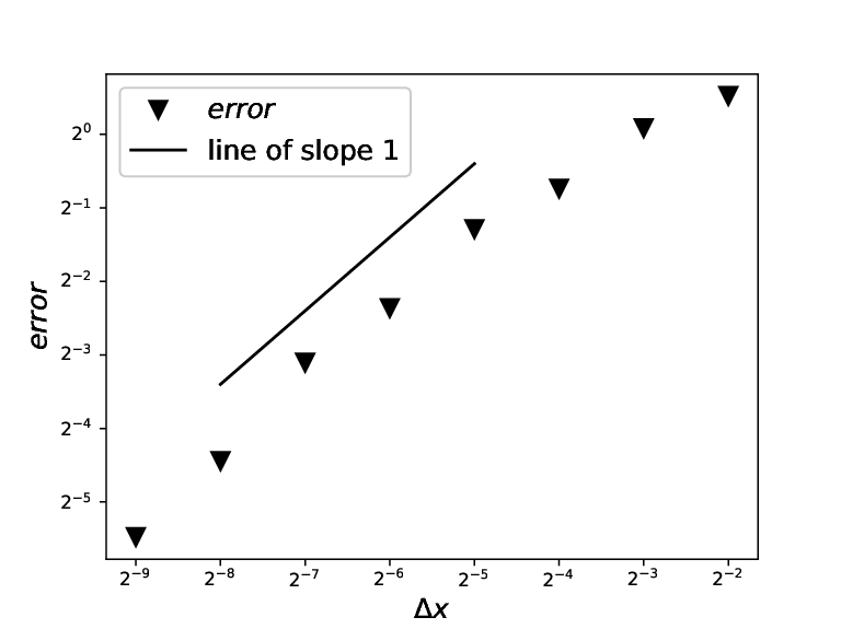
(a) Convergence to benchmark solution for individual diffusion constant ϵ=0.1\epsilon=0.1.
Refer to caption
(b) Convergence to benchmark solution for individual diffusion constant ϵ=0.5\epsilon=0.5.
Figure 3. We choose Gaussian interaction kernels of different strengths and ranges for the self-interaction and the cross-interaction, respectively. The graphs show the numerical convergence order in the cases of ϵ=0.1\epsilon=0.1 (left), and ϵ=0.5\epsilon=0.5 (right), respectively.

6.2. General behaviour of solutions and stationary states

In this section we aim to study the asymptotic behaviour of system (1) numerically. Let us begin by going back to the set up of Section 6.1.2. We note that the potentials were chosen in such a way that there is an attractive intraspecific force, and the cross-interactions are chosen as attractive-repulsive explaining the segregation observed in Figure 4(a). For larger self-diffusivity, ϵ=0.5\epsilon=0.5, we see that some mixing occurs. In the absence of any individual diffusion we would have expected adjacent species with a jump discontinuity at their shared boundary [19]. However, this phenomenon is no longer possible as we have a control on the gradients of each individual species, by Lemma 3.3, rendering jumps impossible thus explaining the continuous transition.

(a) Stationary state (ϵ=0.1\epsilon=0.1).
(b) Stationary state (ϵ=0.5\epsilon=0.5).
Figure 4. We choose Gaussian interaction kernels of different strengths and ranges for the self-interaction and the cross-interaction, respectively. The graphs correspond to the simulationed stationary states for self-diffusivities ϵ=0.1\epsilon=0.1, and ϵ=0.5\epsilon=0.5, respectively.

In the subsequent section we shall push our scheme even further by dropping the smoothness assumption on our potentials.

6.2.1. Case of singular potentials

In this section we go beyond the limit of what we could prove in this paper. On the one hand we consider more singular potentials and on the other hand we consider vanishing individual diffusion. We study system (1) for ϵ∈{0, 0.02, 0.04, 0.06, 0.09}\epsilon\in\{0,\,0.02,\,0.04,\,0.06,\,0.09\}, and ν∈{0.05,0.5}\nu\in\{0.05,0.5\}. Here the potentials are given by

W11​(x)=W22​(x)=x2/2.\displaystyle W_{11}(x)=W_{22}(x)=x^{2}/2.

for the self-interaction terms and

W12​(x)=|x|=±W21​(x).\displaystyle W_{12}(x)=|x|=\pm W_{21}(x).

for the cross-interactions. The system is posed on the domain [0,5][0,5] with a grid size of Δ​x=2−8\Delta x=2^{-8}. Note that the case of ϵ=0\epsilon=0 corresponds to the absence of individual diffusion, see Figures 5(a) & 5(c). By virtue of Corollary 3.3, it is the individual diffusion that regularises the stationary states, in the sense that we will not observe any discontinuities in either ρ\rho or η\eta. As we add individual diffusion we can see the immediate regularisation. While stationary states may still remain segregated, as it is shown in Figure 5(b), adjacent solutions are not possible anymore (see Figure 5(d)).

(a) In the case ν=0.05\nu=0.05, ϵ=0\epsilon=0, we obtain a great agreement of the numerically computed stationary states and the analytical stationary states described in [19].
Refer to caption
(b) Adding individual diffusion may still lead to segregated stationary states. However both species remain continuous as they mix.
(c) The case ν=0.5\nu=0.5, ϵ=0\epsilon=0 leads to adjacent stationary states. Again we see an excellent agreement of the numerical stationary states and the analytical ones [19].
(d) The regularising effect of the individual diffusion, by Corollary 3.3, becomes apparent immediately. Instantaneously both species become continuous as they start to intermingle in a small region. This region grows as we keep increasing the individual diffusion.
Figure 5. We pushed our numerical scheme to see how it performs in regimes in which we are unable to prove convergence. We chose Newtonian cross-interactions in the attractive-repulsive case. The red curves denote the symmetric stationary states of η\eta while the blue curves are the stationary distributions of ρ\rho. The different line widths and styles correspond to varying values of ϵ\epsilon.

In the case of attractive-repulsive interspecific interactions, i.e.

W12​(x)=|x|=−W21​(x).\displaystyle W_{12}(x)=|x|=-W_{21}(x).

we expect both species to segregate [19]. We initialise the system with the following symmetric initial data

ρ⁡(x)=η⁡(x)=c​((x−3)​(5−x))+,\displaystyle\rho(x)=\eta(x)=c\big((x-3)(5-x)\big)^{+},

as symmetric initial data are known to approach stationary states [19]. Here the constant cc normalises the mass of ρ\rho and η\eta to one.

Figures 5(a) & 5(c) show our scheme performs well even in regimes we are unable to show convergence due to the lack of regularity in the potentials as well as the lack of regularity due to the absence of the porous medium type self-diffusion. While the schemes developed in [14, 19] are asymptotic preserving, their convergence to weak solutions of the respective equations could not be established. We reproduce the steady states of [19] that exhibit phase separation phenomena. Figure 6 displays the stationary state in the case ν=0.09\nu=0.09 and ϵ=0\epsilon=0. Even in the case of no regularising individual diffusion and with Newtonian cross-interactions we observe a numerical convergence order of one.

Refer to caption
(a) Strictly segregated stationary state in the absence of individual diffusion, ϵ=0\epsilon=0, and Newtonian potentials.
Refer to caption
(b) Convergence to benchmark solution in the case of ϵ=0\epsilon=0 and Newtonian attractive-repulsive potentials.
Figure 6. Stationary state and numerical convergence order in the case of Newtonian attractive-repulsive cross-interactions. Even though our estimates fail in the analysis above we observe a numerical convergence order of one.

In the case of attractive-attractive cross-interactions, i.e. W12​(x)=|x|=W21​(x)W_{12}(x)=|x|=W_{21}(x), we observe an interesting phenomenon. Even in the absence of the individual diffusion, i.e. ϵ=0\epsilon=0, some additional mixing occurs even though we expect sharp boundaries, see Figure 7, due to numerical diffusion. This is in contrast to the finite volume schemes proposed in [14, 19].

Figure 7. We choose m1=0.6m_{1}=0.6 and m2=0.1m_{2}=0.1 in order to be able to compare the stationary state with the explicit one given in [19]. We can see a strong resemblance between the numerical stationary state and the one obtained analytically. However there are some regimes of mixing due to numerical diffusion.

6.3. Energy dissipation

It is known that system (1) has a formal gradient flow structure, cf. [24], whenever W12=W21W_{12}=W_{21}. In this case, the evolution of system 1 is such that it decays the energy functional

𝔈⁡(ρ,η):=12​∬ρ​W11⋆ρ+η​W22​η​𝑑x+∬ρ​W12⋆η​𝑑x+12​∫ν​(ρ+η)2+ϵ​ρ2+ϵ​η2​𝑑x.\displaystyle\mathfrak{E}(\rho,\eta):=\frac{1}{2}\iint\rho W_{11}\star\rho+\eta W_{22}\eta\,{\rm{d}}x+\iint\rho W_{12}\star\eta\,{\rm{d}}x+\frac{1}{2}\int\nu(\rho+\eta)^{2}+\epsilon\rho^{2}+\epsilon\eta^{2}\,{\rm{d}}x.

Here, we present two examples, one corresponding to the potential

Wi​i​(x)=x22,andWi​j​(x)=|x|,\displaystyle W_{ii}(x)=\frac{x^{2}}{2},\quad\text{and}\quad W_{ij}(x)=|x|,

for i,j=1,2i,j=1,2 and i≠ji\neq j, cf. Figure 8, the other one corresponding to

Wi​i​(x)=1−exp⁡(−(4​x)22),andWi​j​(x)=1+exp⁡(−(4​x)2)−exp⁡(−23​(4​x)2),\displaystyle W_{ii}(x)=1-\exp\left(-\frac{(4x)^{2}}{2}\right),\quad\text{and}\quad W_{ij}(x)=1+\exp\left(-(4x)^{2}\right)-\exp\left(-\frac{2}{3}(4x)^{2}\right),

for i,j=1,2i,j=1,2 and i≠ji\neq j, cf. Figure 9.

In the first case, we choose the initial data

ρ⁡(x)=c​((x−2)​(2.5−x))+,andη⁡(x)=c​((x−1)​(0.5−x))+,\displaystyle\rho(x)=c\big((x-2)(2.5-x)\big)^{+},\quad\text{and}\quad\eta(x)=c\big((x-1)(0.5-x)\big)^{+},

where c>0c>0 normalises the mass to one. Due to the long-range we observe an attraction of the two initial bumps until they meet. They begin to mix until they are completely merged. The graph in the last panel shows the decay of the associated energy to a constant one which corresponds to the energy of the steady state. It appears the energy is dissipated at an exponential rate but an analytic result for systems, corresponding to that of a single equation, cf. [21], is not known to our knowledge.

(a) t=0t=0
(b) t=0.211t=0.211
(c) t=0.433t=0.433
(d) t=0.614t=0.614
(e) t=0.768t=0.768
(f) t=0.909t=0.909
(g) t=1.111t=1.111
(h) t=1.41t=1.41
(i) Decay of the energy, 𝔈⁡(ρ,η)\mathfrak{E}(\rho,\eta).
Figure 8. Evolution of segregated initial data for attractive-attractive interactions with corresponding potentials Wi​i​(x)=x2/2W_{ii}(x)=x^{2}/2 and Wi​j​(x)=|x|W_{ij}(x)=|x|. The two blobs move towards each other. The associated energy appears to converge exponentially fast to a constant while the profiles merge.

In the second case, for Gaussian potentials, we change the computational domain to (0,π)(0,\pi), for convenience. We choose the initial data

ρ⁡(x)=sin⁡(2​x)2,andcos⁡(2​x)2,\displaystyle\rho(x)=\sin(2x)^{2},\quad\text{and}\quad\cos(2x)^{2},

cf. Figure 9. We observe the formation of nearly segregated clusters which, as the evolution continues, as begin to merge due to the nonlocal interaction. However, the short-range cross-interaction is working against this trend which explains that the evolution slows down just before the merging, a phenomenon which is also observed in meta-stability. After the 5 clusters have merged into three the profile stabilises which is reflected in the evolution of the energy, cf. graph in the panel. We still observe a decay, however, after a strong initial decrease the energy decays much slower for a while before going to the constant corresponding to the stationary state. The explanation lies in the increase of the internal energy. Initially, we have ρ+η≡1\rho+\eta\equiv 1 which is a minimiser of the internal energy. Due to the nonlocal interactions the system wants to rearrange but at the cost of increasing the internal energy to allow for a decrease in the interaction energy. This beautifully portrays the interplay of local and nonlocal effects. Similar effects are known in the context of meta-stability.

(a) t=0.0t=0.0
(b) t=1.05t=1.05
(c) t=5.396t=5.396
(d) t=9.89t=9.89
(e) t=10.417t=10.417
(f) t=10.58t=10.58
(g) t=10.71t=10.71
(h) t=19.54t=19.54
(i) Decay of the energy, 𝔈⁡(ρ,η)\mathfrak{E}(\rho,\eta).
Figure 9. Evolution of mixed initial data, ρ=sin⁡(2​x)2\rho=\sin(2x)^{2} and η=cos⁡(2​x)2\eta=\cos(2x)^{2} on the domain (0,π)(0,\pi). The interactions are linear combinations of Gaussians modelling self-attraction whereas the cross-interactions are short-range repulsive and long-range attractive. The associated energy decays abruptly at the merging and separation between aggregates. The slower decay of the energy before t≈10t\approx 10 is due to the trade off between the local (internal) energy and the nonlocal interaction energy. After the rearrangement of the five initial clusters to only three, the energy stabilises.

7. Conclusion

In this paper we presented a finite volume scheme for a system of non-local partial differential equations with cross-diffusion. We were able to reproduce a continuous energy estimate on the discrete level for our scheme. These discrete estimates for the approximate solution are enough to get compactness results and we are able to identify the limit of the approximate solutions as a weak solution of the equation. We complement the analytical part with numerical simulations. These back up our convergence result and we are also able to apply the scheme in cases in which we cannot show convergence. To this end we pushed the scheme to regimes of singular potentials also lacking the regularising porous medium type self-diffusion terms. Comparing them with the explicit stationary states from [19] we conclude the scheme performs well even in regimes it was not designed for.

Acknowledgements

JAC was partially supported by EPSRC grant number EP/P031587/1.

References

  • [1] H. Attouch, G. Buttazzo, and G. Michaille. Variational analysis in Sobolev and BV spaces: applications to PDEs and optimization. SIAM, 2014.
  • [2] J. Berendsen, M. Burger, and J.-F. Pietschmann. On a cross-diffusion model for multiple species with nonlocal interaction and size exclusion. Nonlinear Analysis, 159:10–39, 2017.
  • [3] M. Bertsch, R. Dal Passo, and M. Mimura. A free boundary problem arising in a simplified tumour growth model of contact inhibition. Interfaces and Free Boundaries, 12(2):235–250, 2010.
  • [4] M. Bertsch, M. Gurtin, and H. D. On a degenerate diffusion equation of the form c​(z)t=φ​(zx)xc(z)_{t}=\varphi(z_{x})_{x} with application to population dynamics. Journal of differential equations, 67(1):56–89, 1987.
  • [5] M. Bertsch, M. Gurtin, H. D., and L. Peletier. On interacting populations that disperse to avoid crowding: preservation of segregation. Journal of mathematical biology, 23(1):1–13, 1985.
  • [6] M. Bertsch, M. Gurtin, and D. Hilhorst. On interacting populations that disperse to avoid crowding: the case of equal dispersal velocities. Nonlinear Analysis: Theory, Methods & Applications, 11(4):493–499, 1987.
  • [7] M. Bertsch, D. Hilhorst, H. Izuhara, and M. Mimura. A nonlinear parabolic-hyperbolic system for contact inhibition of cell-growth. Differ. Equ. Appl, 4(1):137–157, 2012.
  • [8] M. Bessemoulin-Chatard, C. Chainais-Hillairet, and F. Filbet. On discrete functional inequalities for some finite volume schemes. IMA J. Num. Analysis, 35(3):1125–1149, 2015.
  • [9] M. Bessemoulin-Chatard and F. Filbet. A finite volume scheme for nonlinear degenerate parabolic equations. SIAM Journal on Scientific Computing, 34(5):B559–B583, 2012.
  • [10] M. Bruna, M. Burger, H. Ranetbauer, and M.-T. Wolfram. Cross-diffusion systems with excluded-volume effects and asymptotic gradient flow structures. Journal of Nonlinear Science, 27(2):687–719, 2017.
  • [11] M. Burger, M. Di Francesco, S. Fagioli, and A. Stevens. Sorting phenomena in a mathematical model for two mutually attracting/repelling species. preprint arXiv:1704.04179, 2017.
  • [12] V. Calvez and J. A. Carrillo. Volume effects in the Keller-Segel model: energy estimates preventing blow-up. J. Math. Pures Appl. (9), 86(2):155–175, 2006.
  • [13] E. A. Carl. Population control in arctic ground squirrels. Ecology, 52(3):395–413, 1971.
  • [14] J. A. Carrillo, A. Chertock, and Y. Huang. A finite-volume method for nonlinear nonlocal equations with a gradient flow structure. Communications in Computational Physics, 17(01):233–258, 2015.
  • [15] J. A. Carrillo, Y.-P. Choi, and M. Hauray. The derivation of swarming models: mean-field limit and wasserstein distances. In Collective dynamics from bacteria to crowds, pages 1–46. Springer, 2014.
  • [16] J. A. Carrillo, A. Colombi, and M. Scianna. Adhesion and volume constraints via nonlocal interactions lead to cell sorting. preprint arXiv:1706.08969, 2017.
  • [17] J. A. Carrillo, S. Fagioli, F. Santambrogio, and M. Schmidtchen. Splitting schemes & segregation in reaction-(cross-)diffusion systems. arXiv preprint arXiv:1711.05434, 2017.
  • [18] J. A. Carrillo, Y. Huang, and S. Martin. Explicit flock solutions for Quasi-Morse potentials. European J. Appl. Math., 25(5):553–578, 2014.
  • [19] J. A. Carrillo, Y. Huang, and M. Schmidtchen. Zoology of a non-local cross-diffusion model for two species. arXiv preprint arXiv:1705.03320, 2017.
  • [20] J. A. Carrillo, S. Martin, and V. Panferov. A new interaction potential for swarming models. Phys. D, 260:112–126, 2013.
  • [21] J. A. Carrillo, R. J. McCann, C. Villani, et al. Kinetic equilibration rates for granular media and related equations: entropy dissipation and mass transportation estimates. Revista Matematica Iberoamericana, 19(3):971–1018, 2003.
  • [22] C. Chainais-Hillairet and F. Filbet. Asymptotic behaviour of a finite-volume scheme for the transient drift-diffusion model. IMA journal of numerical analysis, 27(4):689–716, 2007.
  • [23] X. Chen, A. Jüngel, and J.-G. Liu. A note on Aubin-Lions-Dubinskiĭ lemmas. Acta Appl. Math., 133:33–43, 2014.
  • [24] M. Di Francesco, A. Esposito, and S. Fagioli. Nonlinear degenerate cross-diffusion systems with nonlocal interaction. Nonlinear Analysis, 169:94–117, 2018.
  • [25] M. Di Francesco and S. Fagioli. Measure solutions for non-local interaction pdes with two species. Nonlinearity, 26(10):2777, 2013.
  • [26] P. Domschke, D. Trucu, A. Gerisch, and M. A. J. Chaplain. Mathematical modelling of cancer invasion: implications of cell adhesion variability for tumour infiltrative growth patterns. J. Theoret. Biol., 361:41–60, 2014.
  • [27] M. R. D’Orsogna, Y.-L. Chuang, A. L. Bertozzi, and L. S. Chayes. Self-propelled particles with soft-core interactions: patterns, stability, and collapse. Physical review letters, 96(10):104302, 2006.
  • [28] R. Eymard, T. Gallouët, and R. Herbin. Finite volume methods. Handbook of numerical analysis, 7:713–1018, 2000.
  • [29] R. Eymard, T. Gallouët, and R. Herbin. Finite volume methods. In Handbook of numerical analysis, Vol. VII, Handb. Numer. Anal., VII, pages 713–1020. North-Holland, Amsterdam, 2000.
  • [30] F. Filbet and M. Herda. A finite volume scheme for boundary-driven convection-diffusion equations with relative entropy structure. Numer. Math., 137(3):535–577, 2017.
  • [31] A. Gerisch and M. A. J. Chaplain. Mathematical modelling of cancer cell invasion of tissue: Local and non-local models and the effect of adhesion. Journal of Theoretical Biology, 250(4):684–704, 2008.
  • [32] W. Gurney and R. Nisbet. The regulation of inhomogeneous populations. Journal of Theoretical Biology, 52(2):441–457, 1975.
  • [33] M. E. Gurtin and A. Pipkin. A note on interacting populations that disperse to avoid crowding. Quarterly of Applied Mathematics, 42(1):87–94, 1984.
  • [34] Y. Itô. The growth form of populations in some aphids, with special reference to the relation between population density and the movements. Researches on Population Ecology, 1(1):36–48, 1952.
  • [35] A. Mogilner and L. Edelstein-Keshet. A non-local model for a swarm. Journal of Mathematical Biology, 38(6):534–570, 1999.
  • [36] M. Morisita. Population density and dispersal of a water strider. gerris lacustris: Observations and considerations on animal aggregations. Contributions on Physiology and Ecology, Kyoto University, 65:1–149, 1950.
  • [37] M. Morisita. Dispersion and population pressure: experimental studies on the population density of an ant-lion, glenuroides japonicus m’l (2). Jap. J. Ecol, 4(71):9, 1954.
  • [38] H. Murakawa and H. Togashi. Continuous models for cell–cell adhesion. Journal of theoretical biology, 374:1–12, 2015.
  • [39] K. J. Painter, J. M. Bloomfield, J. A. Sherratt, and A. Gerisch. A nonlocal model for contact attraction and repulsion in heterogeneous cell populations. Bull. Math. Biol., 77(6):1132–1165, 2015.
  • [40] K. J. Painter and T. Hillen. Volume-filling and quorum-sensing in models for chemosensitive movement. Can. Appl. Math. Q., 10(4):501–543, 2002.
  • [41] C. M. Topaz, A. L. Bertozzi, and M. A. Lewis. A nonlocal continuum model for biological aggregation. Bulletin of mathematical biology, 68(7):1601–1623, 2006.
  • [42] A. Volkening and B. Sandstede. Modelling stripe formation in zebrafish: an agent-based approach. Journal of The Royal Society Interface, 12(112), 2015.