Graph Pattern Matching Preserving Label-Repetition Constraints
Abstract
Graph pattern matching is a routine process for a wide variety of applications such as social network analysis. It is typically defined in terms of subgraph isomorphism which is NP-Complete. To lower its complexity, many extensions of graph simulation have been proposed which focus on some topological constraints of pattern graphs that can be preserved in polynomial-time over data graphs. We discuss in this paper the satisfaction of a new topological constraint, called Label-Repetition constraint. To the best of our knowledge, existing polynomial approaches fail to preserve this constraint, and moreover, one can adopt only subgraph isomorphism for this end which is cost-prohibitive. We present first a necessary and sufficient condition that a data subgraph must satisfy to preserve the Label-Repetition constraints of the pattern graph. Furthermore, we define matching based on a notion of triple simulation, an extension of graph simulation by considering the new topological constraint. We show that with this extension, graph pattern matching can be performed in polynomial-time, by providing such an algorithm. Our algorithm is sub-quadratic in the size of data graphs only, and quartic in general. We show that our results can be combined with orthogonal approaches for more expressive graph pattern matching.
AMS
F.2 [Analysis of algorithms and problem complexity]: Nonnumerical algorithms and problems[pattern matching]keywords
Graph pattern matching, triple simulation, Label-Repetition constraint1 Introduction
Modeling data with graphs is one of the most active topics in the database community these days. This model has recently gained wide applicability in numerous domains that find the relational model too restrictive, such as social networks [5], biological networks, Semantic Web, crime detection networks and many others. Indeed, it is less complex and also most natural for users to reason about an increasing number of popular datasets, such as the underlying networks of Twitter, Facebook, or LinkedIn, within a graph paradigm. In emerging applications such as social networks, edges of data graphs (resp. pattern graphs) can be typed [6] to denote various relationships such as marriage, friendship, recommendation, co-membership, etc. Moreover, pattern graphs can define multi-labeled vertices [18] to look, e.g., for persons with different possible profiles.
Given a data graph and a pattern graph , the problem of graph pattern matching is to find all subgraphs of that satisfy both the labeling properties and topological constraints carried by . Matching here is expressed in terms of subgraph isomorphism which consists to find all subgraphs of that are isomorphic to . Graph pattern matching via subgraph isomorphism is an NP-Complete problem as there are possibly an exponential number of subgraphs in that match . To tackle this NP-Completeness, graph simulation [17] has been adopted for graph pattern matching [16] to preserve child-relationships only. Unlike subgraph isomorphism which requires a bijective mapping function from pattern nodes to data nodes, graph simulation is defined by a simple binary relation which can be computed in quadratic time. A cubic-time extension of graph simulation, called strong simulation, has been proposed [14] by enforcing two additional conditions: duality to preserve child and parent relationships of the pattern graph; and locality to overcome excessive matching by considering only subgraphs that have radius bounded by the diameter of the pattern graph.
Nonetheless, the polynomial-time complexity comes at a price: the result of strong simulation may contain incorrect matches as shown below.

Example 1.
Consider the real-life example taken from [14] with minor modification. A headhunter (HR) wants to find a biologist (BIO) to help a group of software engineers (SE) analyze genetic data. To do this, she uses the network depicted in Fig. 1. In , nodes denote persons with different profiles, and edges indicate recommendations between these persons. The cycle between the nodes and contains many DM (data mining specialist) that are all connected to the BIO represented by the node . The biologist BIO to find is specified with the pattern graph of Fig. 1. Intuitively, the BIO has to be recommended by: (a) an HR person since the headhunter trusts the judgment of a person with the same occupation; (b) at least two SE that are recommended by the same HR person (to increase incredibility), that is, the BIO has a strong experience by working with different SEs; and (c) a DM, as data mining techniques are required for the job. Moreover, there is an artificial intelligence expert (AI) who recommends the DM and is recommended by a DM.
When strong simulation is adopted, the subgraph of is returned as the only match of in . However, the BIO of this match, represented by the node , is recommended by only one SE, which is incorrect w.r.t . To make search less restrictive, one can look for a BIO with the same constraints specified by excepting that this BIO can be recommended by only one SE. This search is specified by the pattern graph of the same figure. In this case, strong simulation returns as the only match of in , which is a correct. Notice however that strong simulation does not make difference between and since the two pattern graphs are matched over to the same match result.
The pattern graph illustrates a new kind of topology that we call Label-Repetition (LR) constraint.
Graph simulation [16] and its counterparts [7, 14] fail to preserve this constraint.
One can adopt subgraph isomorphism to preserve LR constraints during graph pattern matching. The challenge is that
subgraph isomorphism is NP-Complete and real-life data graphs are often big, e.g.,
the social graph of Facebook has billions of nodes and trillions of edges [11]. This motivates us to study an extension of
graph simulation in order to preserve LR constraints in polynomial-time.
Contributions & Road-map. Our main contributions are as follows:11
1
The proofs are given in Appendix.
(1) We introduce a new extension of graph simulation, called triple simulation, to preserve LR
constraints (Section 3). (2) We define a necessary and sufficient condition that characterizes the satisfaction
of LR constraints and we compute its time complexity (Section 4). (3) We develop a graph
pattern matching algorithm which requires a polynomial-time to preserve Child and Parent relationships, as well as LR
constraints (Section 5). Finally, we show how to improve the quality of our match results by using the
notion of locality (Section 6).
Related work. We categorize related work as follows.
Polynomial-time graph pattern matching: Traditional matching is by subgraph isomorphism, which is NP-Complete [3] and found often too restrictive to capture sensible matches [7]. To loosen the restriction, one direction is to adopt graph simulation [17]. Matching based on graph simulation [16] preserves only child relationships of the pattern graphs, which makes it useful for some applications like Web sites classification [1]. In other applications however, e.g. social network analysis, the result of such matching may have a structure drastically different from that of the pattern graph, and often very large to analysis and understand. To handle this, strong simulation is proposed [14] to capture child and parent relationships (notion of duality), and to make match results bounded by the diameter of the underlying pattern graph (notion of locality). This approach has proven efficient since it is in PTIME. However, it can not match correctly pattern graphs with LR constraints.
Quantified pattern graphs: Closer to our work is [10] that introduces quantified pattern graphs (QGPs), an extension of pattern graphs by supporting simple counting quantifiers on edges. A QGP naturally expresses numeric and ratio aggregates, and negation besides existential and universal quantification. Notice that any ratio aggregate can be translated into numeric aggregate. Quantified matching is NP-Complete in the absence of negation and DP-Complete for general QGPs. As shown in the Appendix D, any QGP with numeric aggregates can be translated into a simple pattern graph with only LR constraints. This translation allows to preserve numeric and ratio aggregates on edges in polynomial-time, contrary to the prohibitive-cost found by the authors [10]. Furthermore, we think that matching over pattern graphs with negation and universal quantifications on edges can be done in PTIME if treated as an extension of graph simulation (one of our future directions).
2 Background
We give basic notions of graphs and then we review some graph pattern matching approaches.
Graphs. A directed graph (or simply a graph) is defined with () where: 1) is a finite set of nodes; 2) is a finite set of edges in which denotes an edge from nodes to ; and 3) is a labeling function that maps each node to a label in a set of labels. We simply denote as when it is clear from the context.
In this paper, both data graphs and pattern graphs are specified with the previous graph structure. Moreover, we assume that pattern graphs are connected, as a common practice.
Distance and diameter [14]. The distance from nodes to in a graph , denoted by dist(), is the length of the shortest undirected path from to in . The diameter of a connected graph , denoted by , is the longest shortest distance of all pairs of nodes in , that is, = max(dis(, )) for all nodes , in .
Graph pattern matching. A data graph () may match a pattern graph () via different methods.
A) Subgraph isomorphism: A subgraph () of matches via subgraph isomorphism, denoted , if there exists a bijective function : such that: 1) for each node , ; and 2) for each edge , there exists an edge .
B) Graph simulation: matches via graph simulation [16], denoted , if there exists a binary match relation such that:
- 1.
For each , ; and
- 2.
For each node , there exists a node such that: a) ; and b) for each edge , there exists an edge with .
Intuitively, graph simulation preserves only child relationships of the pattern graph.
C) Dual simulation: matches via dual simulation [14], denoted , if there exists a binary match relation such that:
- 1.
For each , ; and
- 2.
For each node , there exists a node such that: a) ; b) for each edge , there exists an edge with ; and moreover c) for each edge , there exists an edge with .
Remark that dual simulation enhances graph simulation by imposing the condition (c) in order to preserve both child and parent relationships. As mentioned in [14], the graph pattern matching via graph simulation (resp. dual simulation) is to find the the maximum match relation (resp. ). Ma et al. [14] show that graph/dual simulation may do excessive matching of pattern graphs which makes the graph result very large and difficult to understand and analysis. For this reason, they propose strong simulation, an extension of dual simulation by imposing the notion of locality. This notion requires that each subgraph of the final match result must have a radius bounded by the diameter of the pattern graph.
D) Strong simulation: matches via strong simulation, denoted , if there exists a node and a subgraph of centered at such that:
- 1.
The radius of is bounded by , i.e., for each node in , dist();
- 2.
with the maximum match relation .
Informally, rather than matching the whole data graph over we extract, for each node , a subgraph of centered at and which has a radius equals to . Then, we match over via dual simulation. In this way, the match result will be composed of subgraphs of reasonable size that satisfy both child and parent relationships of .
Match results. A) When then the match result is the set of all subgraphs of that are isomorphic to . B) When with the maximum match relation then the match result w.r.t is each subgraph () of in which: 1) a node iff it is in ; and 2) an edge iff there exists an edge with and . C) When then the match result is defined similarly to graph simulation but w.r.t the maximum match relation . D) When then the match result is defined with where each is a subgraph of that satisfies the conditions of strong simulation.
Potential matches. Given a data graph () and a pattern graph (). For any node , we call potential match each node that has the same label as (i.e. ). Moreover, sim() refers to the set of all potential matches of in .
Example 2.
Consider the data graph and the pattern graph of Fig. 1. With dual simulation, both and are found as matches of in . Remark that the cycle of two nodes AI and DM in is matched with the long cycle in , which may be hard to analysis. With the notion of locality, strong simulation returns as the only match of over and ignores since it represents an excessive matching.
3 Triple Simulation
We start first by presenting a new topological constraint that one would like to preserve during graph pattern matching. We then define a new extension of graph simulation by imposing this constraint. We compare our extension with only strong simulation [14] since this is the more expressive graph pattern matching approach that requires a polynomial-time. Notice that another polynomial-time approach exists [7], called bounded simulation, which imposes constraints on edges. However, our extension concerns nodes constraints.
Given a data graph and consider the pattern graphs and . It is obvious that these two patterns are not equivalent: requires that each node in that matches must have at least one child node labeled with , however, requires that must have at least two child nodes labeled with . Strong simulation fails to make this difference and considers and as equivalent patterns (as illustrated by Example 1).
Definition 1.
Given a data graph () and a pattern graph (). A Label-Repetition (LR) constraint defined over a node with label specifies that: 1) there is a maximum subset () of children (resp. parents) of that are all labeled with ; and 2) any match of in must have a subset of children (resp. parents) ordered in such a way that allows to match each to a child of .
Intuitively, a LR constraint concerns a repetition of some label either among children or among parents of some node in . If children (resp. parents) of each node in have distinct labels, then is defined with only child and parent relationships and, thus, can be matched correctly via strong simulation. The limitation of this latter is observed when some children (resp. parents) of the same node are defined with the same label.
Example 3.
Consider the pattern graph of Fig. 1. There is an LR constraint defined over the node with label SE. It specifies that each node of the data graph that matches must have at least two children labeled SE such that one of them matches the node and the other one matches the node .
We propose next a new extension of graph simulation in order to satisfy LR constraints.
Definition 2.
A data graph matches a pattern graph via triple simulation, denoted by , if there exists a binary match relation s.t.:
- 1.
For each , .
- 2.
For each there exists .
- 3.
For each and for all edges , there exists at least distinct children of in such that: .
- 4.
For each and for all edges , there exists at least distinct parents of in such that: .
is the match result that corresponds to the maximum match relation 22 2 This match result can be defined similarly to graph (dual) simulation..
Intuitively, if a node in has children (resp. parents) then each match of in must have at least distinct children (resp. parents) such that we can match, w.r.t some order, each child (resp. parent) of to only one child (resp. parent) of . This new restriction imposed by conditions (3) and (4) prevents matching of distinct children (resp. parents) of some node in to the same node in , as may be done by strong simulation. Notice that triple simulation preserves also child and parent relationships and not only LR constraints.
Example 4.
Consider the data graph and the pattern graphs and of Fig. 1. The node with label BIO in has two parents, and , that have the same label SE. Remark that and are potential matches of in . According to triple simulation, (resp. ) must have at least two distinct parents s.t. one can match and the other one can match . This is not the case since (resp. ) has only one parent labeled SE. Thus, we can conclude that no subgraph in satisfies the LR constraint of , and then, . When triple simulation is adopted for over the subgraph , we obtain the following maximum match relation: . The match result that corresponds to is the whole subgraph , which is correct.
We use CPL relationships to refer to Child and Parent relationships (called duality properties), as well as relationships based on LR constraints. Our motivation is to popose a graph pattern matching algorithm that preserves CPL relationships in polynomial-time.
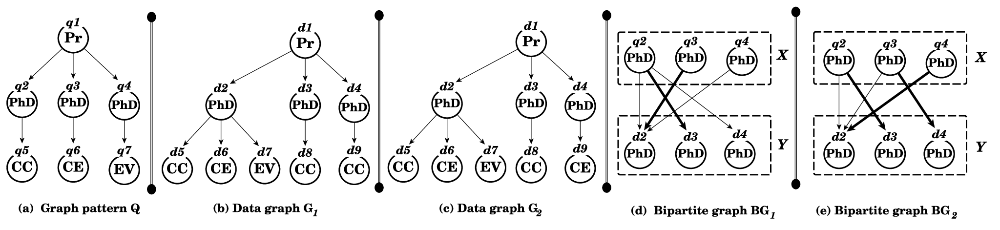
4 Satisfy LR Constraints
We first present the problem of satisfying LR constraints and show that a naive approach may lead for exponential cost. Next, we define a condition that is necessary and sufficient for the satisfaction of LR constraints and which can be checked in polynomial-time.
Example 5.
Consider the graphs depicted in Fig. 2. The pattern graph looks for each professor (Pr) which has supervised at least three PhD thesis in topics related respectively to Cloud Computing (CC), Collaborative Editing (CE) and Electronic Vote (EV). The node in is a potential match of . To satisfy the condition (3) of triple simulation (Definition 5), must have at least three child nodes which is the case, and there must be some order that allows to match each child of to a child of . However remark that: if we match with then we can not have match neither for nor for ; and moreover, if we match with then we can match either with or with . Clearly, there is no order over the children of that allows to match all the children of in . Therefore, the data graph does not satisfy the LR constraint of . On the other side, the data graph match correctly : see that there is an order that allows to match each child of to a child of , i.e., can be matched respectively with . Thus, the LR constraint of is satisfied over .
Given the aboves, one can think that checking LR constraints may lead to exponential cost (since we must consider all orders over some data nodes). However, we show later that this process can be done in polynomial-time.
Definition 3.
Given a data graph () and a pattern graph (). Consider all the LR constraints defined over children (resp. parents) of some node , and let be a potential match of . The bipartite graph () that inspects these LR constraints w.r.t is defined as follows:
- •
contains each child (resp. parent) of that is concerned by an LR constraint.
- •
contains each child (resp. parent) of that (potentially) matches some node in .
- •
if is (potentially) matched with .
A complete matching over is a maximum matching [4] that covers each node in 33 3 It is also called X-saturating matching..
Consider only the LR constraints defined over children of . The set of the bipartite graph contains all children of that are concerned by some LR constraint, and the set contains each child of that (potentially) matches some child of , provided that is concerned by an LR constraint (i.e. ). Moreover, an edge in denotes some child of in that can be (potentially) matched with some child of in . For LR constraints defined over parents of , the bipartite graph that inspects them is defined in the same manner (i.e. is a subset of parents of , and is a subset of parents of ).
Example 6.
Consider the pattern graph and data graphs and depicted in Fig. 2. Recall that there is an LR constraint defined over the children of the node in . The bipartite graph that inspects this LR constraint, w.r.t the potential match of in , is depicted in Fig. 2 (d). Moreover, w.r.t the potential match of in , the corresponding bipartite graph is given in Fig. 2 (e).
The next theorem states our main contribution which is a necessary and sufficient condition to satisfy LR constraints.
Theorem 1.
Given a data graph (), a pattern graph (), and a node with a potential match . Let be the bipartite graph that inspects all the LR constraints defined over children (resp. parents) of w.r.t . These LR constraints are satisfied by some children (resp. parents) of iff there is a complete matching over . Moreover, this can be decided in at most time.
We emphasize that for each node in and each potential match of in , we construct at most two bipartite graphs, the first one to inspect LR constraints that are defined over children of , and the second one to inspects those defined over parents of .
Example 7.
As explained in Example 5, the LR constraint defined over the children of in is not satisfied by the children of its potential match in . This is confirmed by the bipartite graph of Fig. 2 (d) which has a maximum matching of size (does not cover the set ). Thus, no complete matching exists over and, according to Theorem 1, we can conclude that the underlying LR constraint is not satisfied by the children of . Consider the bipartite graph of Fig. 2 (e) that inspects the same LR constraint w.r.t the potential match of . Bold edges in represent a maximum matching of size . Thus, a complete matching exists over which implies that the LR constraint, defined over the children of in , is satisfied by the children of its potential match of .
5 An Algorithm for Triple Simulation
Our algorithm, referred to as TSim, is shown in the Fig. 3. Given a pattern graph and a data graph , TSim() returns the match result , if , and otherwise. This match result contains each subgraph of that satisfies all CPL relationships of .
First, we compute for each node , the set of all its potential matches in [lines 1-3]. In order to preserve efficiently the CPL relationships of over , we define four auxiliary structures [line 4] as follows. For any node , CP() contains all children and parents of that are concerned by Child and/or Parent relationships; and LR() contains those concerned by some LR constraints. Moreover, for each potential match of in , ChildAsMatch() returns the number of ’s children that are potential matches of in (i.e. each child of with ); and ParentAsMatch() returns the number of ’s parents that are potential matches of in .
Algorithm TSim preserves the Child and Parent relationships of [lines 6-15] as follows. Given a node , a potential match of is kept in unless: 1) has a child but has no child that matches (i.e. ChildAsMatch()=0); or 2) has a parent but has no parent that matches (i.e. ParentAsMatch()=0). If one of these two conditions is satisfied then is an incorrect match of , w.r.t duality properties, and is removed from [lines 8 + 13]. The checking of LR constraints [lines 17-19] is done through the procedure LR_Checking. Given a node with a potential match . According to Definition 3, the procedure LR_Checking constructs two bipartite graphs: that inspects all the LR constraints defined over the children of [lines 2-5]; and that inspects those defined over the parents of [lines 6-9]. If a complete matching exists over and another one exists over then, according to Theorem 1, we conclude that: a) all the LR constraints defined over the children of are satisfied by some children of ; and b) all the LR constraints defined over the parents of are satisfied by some parents of . Thus, the procedure returns only if these two complete matching exist over and . If the procedure returns then there is at least one LR constraint defined over the children (resp. parents) of which is not satisfied by the children (resp. parents) of . In this case, is an incorrect match of , w.r.t LR constraints, and is removed from [line 18]. The procedure CompleteMatch44 4 This procedure finds the maximum matching over (resp. ), using the algorithm of Hopcroft et al. [13], and then checks whether the size of this maximum matching is equals to (resp. ). is an implementation of the algorithm of Hopcroft and Karp [13].
Each time a data node is removed from , the cardinalities stored by the structures ChildAsMatch and ParentAsMatch are updated according to the couple . This is done by the procedure UpdateStruct. The two phases discussed above (checking of duality properties and LR constraints) are repeated by algorithm TSim until there are no more changes [lines 5-22]. Finally, the maximum match relation that corresponds to Definition 5 is defined, and its corresponding match result is constructed and returned.
Theorem 2.
For any pattern graph () and data graph (), algorithm TSim takes at most time to decide whether and to find the match result . Moreover, it takes time if has no LR constraint.55 5 Given a graph (), .
The worst-case time complexity of TSim is bounded by . As opposed to the NP-Completeness of its traditional counterpart via subgraph isomorphism [10], triple simulation allows to match pattern graphs with LR constraints in polynomial-time.
Algorithm TSim(, )
Input: Graph pattern (), data graph ().
Output: The match result if and otherwise.
Procedure UpdateStruct()
Input: A pattern graph , data graph (), a query node with a removed potential match .
Output: Updates the auxiliary structures ChildAsMatch and ParentAsMatch.
Procedure LR_Checking()
Input: Graph pattern , data graph , a node with a potential match .
Output: Whether all the LR constraints defined over are satisfied by children and/or parents of .
6 Triple Simulation with Locality
The next example suggests to incorporate the notion of locality [14] into our algorithm TSim in order to overcome excessive matching and thus to improve the quality of our match results.
Example 8.
Consider the graphs depicted in Fig. 1. We extend the subgraph with the following relationships: where is a new node labeled with SE. Let be the subgraph that results from this modification. When triple simulation is adopted, TSim returns as the only match of in . The BIO found in (node ) is recommended by two SE ( and ) as specified by . However, TSim returns an excessive match of the cycle , i.e. the cycle in , that one does not want.
Next is a new definition of triple simulation that takes into account the notion of locality.
Definition 4.
A data graph matches a pattern graph via triple simulation and under locality, denoted , if there exists a subgraph of centered at some node s.t.:
- 1.
the radius of is bounded by , i.e., for each node in , dist(); and
- 2.
with the maximum match relation .
The match result is defined with where each is a subgraph of that satisfies the previous conditions.
To implement the Definition 4, one can replace only the procedure dualSim in the algorithm Match [14] with our algorithm TSim. Let Match+ be the algorithm that results from this combination. Given a data graph and a pattern graph . Algorithm Match+66 6 Not given here since its definition is trivial. extracts a subgraph over each node in , provided that its radius does not exceed . It then matches over via triple simulation (instead of dual simulation). The match found on each subgraph has a reasonable size and satisfies all the CPL relationships of .
Theorem 3.
77 7 This result is a combination of Theorem 2 and Theorem 4.1 of Ma et al. [14].For any pattern graph () and data graph (), algorithm Match+ takes at most time to decide whether and to find the corresponding match result .
The complexity of Match+ is bounded by while that of Match[14] is bounded by . This promises that combining our results with existing orthogonal approaches will not increase drastically the complexity of graph pattern matching.
7 Conclusion
We have discussed pattern graphs with LR constraints that existing approaches do not preserve [14, 7] or preserve in exponential time [10]. To tackle this NP-Completeness, we have showed that LR constraints can be preserved in polynomial-time when treated as maximum matching in bipartite graphs, and we proposed an algorithm to implement this result.
We are to stduy other constraints that can be preserved in polynomial-time, e.g., negation and optional edges. The polynomial-time of our algorithm may make graph pattern matching infeasible when conducted on graphs with millions of nodes and billions of edges (e.g. Facebook [11]). To boost the matching on large data graphs, we plan to extend our work with some optimization techniques: 1) incremental graph pattern matching [9], 2) pattern matching on distributed data graphs [2, 20, 19], and 3) pattern matching on compressed data graphs [8, 15]. These techniques are orthogonal, but complementary, to our work.
References
- [1] Junghoo Cho, Narayanan Shivakumar, and Hector Garcia-Molina. Finding replicated web collections. In Proc. of SIGMOD, pages 355–366, 2000.
- [2] Gao Cong, Wenfei Fan, and Anastasios Kementsietsidis. Distributed query evaluation with performance guarantees. In Proc. of SIGMOD, pages 509–520, 2007.
- [3] Luigi P. Cordella, Pasquale Foggia, Carlo Sansone, and Mario Vento. A (sub)graph isomorphism algorithm for matching large graphs. IEEE Trans. Pattern Anal. Mach. Intell., pages 1367–1372, 2004.
- [4] Thomas H. Cormen, Charles E. Leiserson, Ronald L. Rivest, and Clifford Stein. Introduction to Algorithms, Third Edition. The MIT Press, 3rd edition, 2009.
- [5] Wenfei Fan. Graph pattern matching revised for social network analysis. In Proc. of ICDT, pages 8–21, 2012.
- [6] Wenfei Fan, Jianzhong Li, Shuai Ma, Nan Tang, and Yinghui Wu. Adding regular expressions to graph reachability and pattern queries. In Proc. of ICDE, pages 39–50, 2011.
- [7] Wenfei Fan, Jianzhong Li, Shuai Ma, Nan Tang, Yinghui Wu, and Yunpeng Wu. Graph pattern matching: From intractable to polynomial time. Proc. VLDB Endow., pages 264–275, 2010.
- [8] Wenfei Fan, Jianzhong Li, Xin Wang, and Yinghui Wu. Query preserving graph compression. In Proc. of SIGMOD, pages 157–168, 2012.
- [9] Wenfei Fan, Xin Wang, and Yinghui Wu. Incremental graph pattern matching. ACM Trans. Database Syst., pages 18:1–18:47, 2013.
- [10] Wenfei Fan, Yinghui Wu, and Jingbo Xu. Adding counting quantifiers to graph patterns. In Proc. of SIGMOD, pages 1215–1230, 2016.
- [11] Ivana Grujic, Sanja Bogdanovic Dinic, and Leonid Stoimenov. Collecting and analyzing data from e-government facebook pages. In Proceedings of ICT Innovations, pages 86–96, 2014.
- [12] P. Hall. On representatives of subsets. Journal of the London Mathematical Society, s1-10(1):26–30, 1935.
- [13] John E. Hopcroft and Richard M. Karp. An n5/2 algorithm for maximum matchings in bipartite graphs. SIAM J. Comput., 2(4):225–231, 1973.
- [14] Shuai Ma, Yang Cao, Wenfei Fan, Jinpeng Huai, and Tianyu Wo. Strong simulation: Capturing topology in graph pattern matching. ACM Trans. Database Syst., 39(1):4:1–4:46, 2014.
- [15] Antonio Maccioni and Daniel J. Abadi. Scalable pattern matching over compressed graphs via dedensification. In Proc. of SIGKDD, pages 1755–1764, 2016.
- [16] R. Milner. Communication and Concurrency. Prentice-Hall, Inc., 1989.
- [17] Robin Milner. Communication and concurrency. Prentice Hall, 1989.
- [18] Ali Shemshadi, Quan Z. Sheng, and Yongrui Qin. Efficient pattern matching for graphs with multi-labeled nodes. Knowl.-Based Syst., 109:256–265, 2016.
- [19] Le-Duc Tung, Quyet Nguyen-Van, and Zhenjiang Hu. Efficient query evaluation on distributed graphs with hadoop environment. In Proc. of SoICT, pages 311–319, 2013.
- [20] Xin Wang, Junhu Wang, and Xiaowang Zhang. Efficient distributed regular path queries on RDF graphs using partial evaluation. In Proc. of CIKM, pages 1933–1936, 2016.
APPENDIX
Appendix A Proof of Theorem 1.
Theorem 1. (Recall)
Given a data graph (), a pattern graph (), and a node with a potential match .
Let be the bipartite graph that inspects all the LR constraints defined over children (resp. parents) of
w.r.t . These LR constraints are satisfied by some children (resp. parents) of iff there is a complete matching over .
Moreover, this can be decided in at most time.
To simplify the proof, we consider only the case of LR constraints defined over children of . The second case, i.e. when parents of are concerned by some LR constraints, can be studied in the same way. Satisfying LR constraints is closer to the problem of perfect matching in bipartite graph [4], or moreover, a System of Distinct Representatives [12]. In our case, node sets and of our bipartite graphs have not the same size then we use the term of complete matching instead of perfect matching. Given a bipartite graph =(). A maximum matching is the largest subset of the edge set such that no two edges start/end at the same node. If is a complete matching, i.e. , then for each node there is one and only one edge that connects it with a node . We say that all elements of are covered (i.e. matched).
Consider that all LR constraints defined over children of are satisfied by some children of its potential match . Recall that is defined with where contains each child of that is concerned by an LR constraint; and contains each child of that matches at least one child of in . Let be the number of ’s children that are concerned by LR constraints (i.e. ). Since all the LR constraints in question are satisfied by some children of then, for each single one defined over the subset of children of (), satisfies condition (2) of Definition 1 and has a subset of children such that each matches a child of . Notice that two different LR constraints are defined with two different labels, thus children of that satisfy one LR constraint are different from those that satisfy another LR constraint. By following the same principle, to satisfy all LR constraints defined over children of , has certainly distinct children such that each one is matched to only one child of which is concerned by some LR constraint. This matching can be represented by edges that connect each child of in to only one child of in (*). Moreover, if two children of has the same label then they are concerned by the same LR constraint and, according to Definition 1, are matched to different nodes in (**). From (*) and (**), we conclude that these edges do not start/end at the same node and then represent a complete matching over the bipartite graph . Therefore, if all LR constraints defined over children of are satisfied by some children of , then there is a complete matching over the bipartite graph that inspects these LR constraints w.r.t .
Consider that there is a complete matching over the bipartite graph . According to our definition of complete matching, there is an edge that connects each node in (i.e. a child of that is concerned by an LR constraint) to only one node in (i.e. a child of with ), and moreover, each node in is connected to only one node in . We conclude that has at least children () and there exists an order over these children that allows to match each one to only one child of which is concerned by some LR constraint. Therefore, according to Definition 1, each LR constraint defined over some children of is satisfied by some children of .
The node set (resp. ) of the bipartite graph may have at most (resp. ) nodes. Moreover, the edge set may have at most edges. To check whether there exists a complete matching over , we look first for the maximum matching over and we then check whether its cardinality is equals to . The best algorithm to find a maximum matching over a bipartite graph with node set and edge set , discovered by Hopcroft and Karp [13], runs in time. Thus, by using this algorithm, the necessary and sufficient condition of Theorem 1 can be checked in at most time.
Appendix B Proof of Theorem 2.
Theorem 2. (Recall)
For any pattern graph () and data graph (), algorithm TSim takes at most
time to decide whether and to find the
match result . Moreover, it takes time in the absence of LR constraints.
Given a pattern graph () and a data graph ().
It takes time to compute sim sets for all query nodes of [lines 1-3]. We define each sim() as an indexed
structure which allows, in constant time, 1) to check whether some data node belongs to ; or 2) to remove it from
.
(A) The auxiliary structures CP and LR can be constructed in at most time as follows. For any node , we define an indexed list LabelOcc() which returns the number of children of that are labeled with . This list can be constructed in time by parsing all children of . For each child of , if LabelOcc(), then other children of have the same label as . Thus, is concerned by an LR constraint and must belong to LR(). Otherwise, i.e. LabelOcc(), is the unique child of that has the label and thus must belong to CP(). This process is repeated similarly over parents of to complete the definition of CP() and LR(). It is clear that for each node , CP() and LR() can be constructed in time. Therefore, for all nodes of , the cost becomes .
(B) It is easy to verify that for each query node and data node , ChildAsMatch() (resp. ParentAsMatch()) can be constructed in time by parsing each child (resp. parent) of and checking, in constant time, if this child belongs to . Therefore, by considering all nodes of and , the structures ChildAsMatch and ParentAsMatch can be constructed in at most time.
(C) In addition to the four auxiliary structures described above, we construct in time (resp. time) an indexed structure over the edges of (resp. ) in order to check in constant time whether some data edge (resp. query edge) exists. Moreover, we define sets of children and parents of each query node (resp. data node ) which can be done in time (resp. time).
From (A), (B) and (C), we conclude that the cost of the call initAuxStruct() [line 4]
remains bounded by .
Each time we remove some data node from , the procedure UpdateStruct() of Fig. 3 takes
time
to update the structures ChildAsMatch and ParentAsMatch. This remove operation can be done at most time. Thus,
the lines [9+14+18] of algorithm TSim take at most time.
Given a query node with a potential match . The checking of Child relationships [lines 7-11], as well as Parent relationships [lines 12-16] is done in at most time by using the indexed structures ChildAsMatch and ParentAsMatch (inspired from [16]). Recall that the cost necessary to update these indexed structures is computed separately.
Procedure MatchResult(, , )
Input: A pattern graph , a data graph , and the maximum match relation for which .
Output: The match result that corresponds to .
The call LR_Checking() [line 17] is done in at most time as we explain hereafter. As depicted by the procedure LR_Checking of Fig. 3, we construct first two bipartite graphs and that inspect the LR constraints defined over children of [lines 2-5] and those defined over parents of respectively [lines 6-9]. We get all children/parents of in at most time by using our precomputed sets of children and parents. Thus, the construction of as well as requires a time bounded by . Next, we use the procedure CompleteMatch (not detailed here) to check whether there exist two complete matchings over and respectively. Our bipartite graphs have at most nodes and edges. According to Theorem 1, the existence of complete matching over and can be checked in at most time. Therefore, the checking of LR constraints by algorithm TSim [lines 17-19] requires a time bounded by .
For a query node with a potential match , the checking of duality properties takes time while that of LR constraints takes time. This tells us that the worst case arises when children (resp. parents) of are concerned by only LR constraints. The checking process [lines 6-21] over all potential matches of is done in at most time, in case of duality properties only, and in time in case of LR constraints only.
Inspired from [16], the checking process (of duality properties and LR constraints) [lines 5-22] is executed over the nodes of in a deterministic manner: first over a randomly-chosen query node , after over adjacent nodes of (children and parents) and so on. In this way, each time some sim set is changed we repeat the checking process over all already visited nodes since this change may influence on their sim sets. Thus, the Do-While loop will repeat the checking process times over each query node in .
The definition of the maximum match relation [line 23] can be done in at most time.
The match result that corresponds to can be defined in at most time [line 24].
To proof this cost, we give in Fig. 4 the procedure MatchResult which defines the match result that corresponds
to some maximum match relation. The first For-Each loop of this procedure takes time since the size of is
bounded by .
The second For-Each loop is repeated time, and in each iteration,
we make all combinations between children of and those of , which
takes time. We suppose that it can be checked in constant time whether (resp. ). Thus,
the overall time complexity of the procedure MatchResult remains bounded by .
Hereafter a summary of all the above-mentioned costs of algorithm TSim:
- •
time to compute all sim sets.
- •
time for the call of initAuxStruct.
- •
time for the calls of UpdateStruct.
- •
time for checking of LR constraints, and time for checking of duality properties.
- •
time for the definition of the match result .
For any pattern graph () and data graph () in practice, we have . Thus, the cost can be bounded by . Moreover, (resp. ) is bounded by (resp. ).
Finally, we conclude that the overall time complexity of algorithm TSim is bounded by is case of only duality properties, and by in presence of LR constraints.
Appendix C Proof of Theorem 3
Theorem 3. (Recall)
For any pattern graph () and data graph (), algorithm Match+ takes
at most time to decide whether and to find the corresponding match
result .
Given a pattern graph () and a data graph (). Ma et al. [14] show that their algorithm Match requires time to decide whether and to find the match result . Here DualSimCost denotes the cost of dual simulation since they preserve only child and parents relationships besides the notion of locality. Recall that Match+ is a new version of Match that we propose in order to take advantage of triple simulation as well as of locality, and this by replacing the dual simulation in algorithm Match with triple simulation. More precisely, we replace the procedure DualSim in algorithm Match with our algorithm TSim. Therefore, to get the result of Theorem 3, one can replace intuitively DualSimCost with the overall cost of algorithm TSim (Theorem 2).
Appendix D Discussion about Quantified Graph Patterns
Authors of [10] propose a new extension of subgraph isomorphism by supporting simple counting quantifiers (CQs) on edges. These CQs can express universal and existential quantification, numeric and ratio aggregate, as well as negation.
Example 1.
The pattern graph looks for each professor such that all her PhD students (universal quantification) have at least one conference paper (existential quantification). The pattern graph looks for each professor such that of her PhD students (aggregate ratio) have at least two conference papers (numeric ratio) that are not indexed in DBLP (negation).
Definition 2.
A pattern graph with counting quantifiers, called quantified pattern graph (QGP), is defined with () where , , and are the same as their conventional counterparts; and is a function such that, for each edge , is given by: “”, “”, “”, or “” ().
Remark that conventional pattern graphs are a special case where for each edge , (only existential quantification). We omit from each edge if it is an existential quantification.
It is clear to see that LR constraints are much close to counting quantifiers with numeric aggregate (denoted shortly CQs+). Hence, we conduct in the next a comparison between LR constraints and CQs+ and we show how to extend our algorithm TSim to handle pattern graphs with CQs+. Since the other forms of CQs are not too close to our problem, we consider in the next quantified pattern graphs with only numeric aggregates.

D.1 LR Constraints v.s. CQs+
The limit of CQs+ is that they specify the minimum number of children which must have all the same properties (child clone). Formally, given the edge of some pattern graph . This specifies that: 1) each data node , that matches , must have at least child nodes that match ; and 2) all these nodes must satisfy the same properties set that are defined over in . Moreover, CQs+ are defined over children only.
An LR constraint, however, specifies the minimum number of children or parents that has some query node such that they have all the same label but not necessarily the same properties. In addition, any CQ+ can be transformed to an LR constraint (Proposition 4), but the inverse is not always possible as shows the next example.
Example 3.
Consider the pattern graphs , , , and the data graph depicted in Fig. 5. The pattern graph looks for each professor (Pr) which has supervised: 1) at least two master students (MS) who have worked in the Cloud Computing (CC) area; and 2) at least two PhD students who had topics related to Collaborative Editing (CE) and Electronic Vote (EV) respectively. Remark that is composed by one LR property and one CQ+. This CQ+ can be easily replaced by an LR constraint as follows: we replace the global child node by two copies of it, and , such that the properties defined in over (child of type CC) must be duplicated over each copy of it. This transformation yields for the pattern graph . See that and are equivalent: by using the algorithm in [10], the matching of over returns the whole data graph as match result, which is the same result returned by TSim(). However, it is clear that the LR constraint of can not be replaced by the CQ+ “” as done with the pattern graph . Thus, and are not equivalent: matching over with the algorithm in [10] yields for an empty set.
Proposition 0.
Given a quantified pattern graph (), a data graph (), and a node with a potential match . Each CQ+ defined with over some child of can be transformed into an LR constraint. Moreover, children of satisfy this CQ+ iff they satisfy its equivalent LR constraint.
In the following, we give another definition of triple simulation that takes into account CPL relationships as well as CQs+. We show later that implementing this new definition requires just a simple extension of algorithm TSim.
Definition 5.
Given a data graph and a quantified pattern graph where defines only CQs+. Then, matches via triple simulation, denoted by , if there exists a binary match relation s.t.:
- 1.
For each , .
- 2.
For each there exists .
- 3.
For each and for all simple edges , there exists at least distinct children of in such that: .
- 4.
For each and for all simple edges , there exists at least distinct parents of in such that: .
- 5.
For each and for each edge in with =“”, there exists at least distinct children of in such that: .
is the match result that corresponds to the maximum match relation 88 8 Each subgraph in this match result satisfies CPL relationships as well as CQs+ of ..
Intuitively, we enhance the old definition of triple simulation with the condition (5) in order to preserve CQs+ of . This condition requires that, for each edge in , each match of in must have at least distinct children that match all the child of .
Procedure LR_Checking()
Input: A QGP with only CQs+, a data graph , a node with a
potential match .
Output: Whether LR constraints and CQs+ defined over are satisfied by children and/or parents of .
D.2 Adapting TSim for CQs+
Given a quantified pattern graph () where represents only CQs+. A new definition of the procedure LR_Checking is given in Fig. 6 in order to handle CQs+. Given a query node with a potential match . As explained above, we construct two bipartite graphs and that inspect the LR constraints defined over children and parents of respectively. Recall that CQs+ are defined over children only. Thus, the equivalent LR constraint of each one is defined and included in [lines 6-14]. For each child of that is concerned by a CQ+ of cardinality [line 6], we create copies of in [line 7]. Each potential match of is also a potential match of each copy of . For this reason, 1) we add into each child of that matches the child of ; and 2) we create an edge between each copy and to say that this copy can be matched by . The resulting bipartite graph inspects: 1) the LR constraints defined over children of ; and 2) each LR constraint that results from the transformation of a CQ+ defined over some child of . If a complete matching exists over then all these LR constraints are satisfied by children of , i.e. all CQs+ defined over children of are also satisfied (Proposition 4).

Example 5.
Consider the quantified pattern graph and the data graph depicted in side (a) and (b) of Fig. 7 respectively. It is clear to see that the LR constraint, defined over the children and of , is satisfied over : by matching , , with , , and respectively. However, the CQ+ “” is not satisfied. The match of must have at least two child nodes such that: each one is labeled with and have a child node labeled with . Consider the couple , the bipartite graph constructed by the new procedure LR_Checking is given in Fig. 7 (c). See that two copies of are created ( and ) and each one is connected to the unique match of . Since there is no complete matching over , the procedure returns which means that the LR constraint and the CQ+, that are defined over children of , are not all satisfied by children of .
The next result states that the problem of matching pattern graphs with numeric aggregates is in PTIME when it is treated as an extension of graph simulation, contrary to the NP-Completeness found in [10] when the problem is studied under subgraph isomorphism.
Theorem 6.
Given a data graph () and a quantified pattern graph () where defines only CQs+. Let be the largest cardinality of numeric aggregates . Algorithm TSim takes at most time to decide whether and to find the match result .
Here algorithm TSim uses the new version of procedure LR_Checking given in Fig. 6. The overall time complexity of algorithm TSim, in case of pattern graphs with numeric aggregates, is bounded by where is bounded as follows: .