A Mixed Discrete–Continuous Fragmentation Model
Abstract.
Motivated by the occurrence of “shattering” mass-loss observed in purely continuous fragmentation models, this work concerns the development and the mathematical analysis of a new class of hybrid discrete–continuous fragmentation models. Once established, the model, which takes the form of an integro-differential equation coupled with a system of ordinary differential equations, is subjected to a rigorous mathematical analysis, using the theory and methods of operator semigroups and their generators. Most notably, by applying the theory relating to the Kato–Voigt perturbation theorem, honest substochastic semigroups and operator matrices, the existence of a unique, differentiable solution to the model is established. This solution is also shown to preserve nonnegativity and conserve mass.
Key words and phrases:
Fragmentation models, mixed discrete–continuous fragmentation model, substochastic semigroups, existence and uniqueness of solution2010 Mathematics Subject Classification
35F10, 45K05, 47D06, 47N201. Introduction
The mathematical modelling of fragmentation, and the reverse coagulation process have a long history, with the first work dating back to [1]. Such models have found applications in areas as diverse as polymer science [2], population dynamics [3] and astrophysics [4]. The models of such processes typically classify the entities within the system according to some physical state variable, for example their volume, area or mass, the aim being then to determine the evolution of the system with respect to this variable as time progresses. Models are typically classified as either discrete or continuous, depending on the nature of the state variable of interest. Generally, there are great similarities between the two forms, with each continuous model having an analogous discrete version and vice versa. The selection of the form to use is largely a modelling choice, and depends on the scale of the phenomenon to be described.
In this paper we shall be exclusively considering fragmentation processes, with no coagulation mechanism involved. With continuous models of such processes, difficulties can arise when the break-up rate for particles blows up as their size goes to zero and particles are allowed to get too small too quickly. The unbounded fragmentation rate can result in a runaway fragmentation process and a loss of mass unaccounted for in the model formulation. This loss of mass was observed by McGrady and Ziff in [5], the process was termed ‘shattering’ and attributed to the creation of ‘dust’ particles with zero size but positive mass.
In [6], Huang et al. suggest that such a runaway fragmentation process is unphysical, and that at some point particles become too small to break-up any further. Their proposed model includes a cut-off size , above which particles are able to fragment as usual. However, once a particle’s size drops below it ceases to be able to fragment, becoming dormant. In this paper we shall present a variation on this theme, introducing a mixed discrete–continuous model as a solution to the problem of shattering.
Considering the nature of the material that is undergoing fragmentation that we are attempting to model, on close inspection we might expect there to be some minimum fundamental unit (monomer) from which all particles are built up. Whatever level this occurs at, once this is imposed, the runaway fragmentation, associated with shattering, is prohibited. Such a framework necessarily induces a discrete nature on the material and suggests the use of a discrete model. However, on larger scales where a typical particle is composed of a large number of such monomers and hence where the mass of a particle is highly divisible, the continuum model may provide an adequate and convenient representation. With our hybrid model we attempt to reconcile these factors.
In our model, the smaller particles are considered to be comprised of collections of monomers. Through suitable scaling, the monomers can be assumed to have unit mass and therefore the smaller particles take positive integer mass, up to some cut-off value . However, above this cut-off particle mass is considered as a continuous variable. A set-up such as this produces a dual regime model, with a discrete mass regime below the cut-off and a continuous mass regime above.
Let us denote by the particle mass density within the continuous mass regime. The evolution of is then governed by the continuous multiple fragmentation equation below:
| (1.1) | ||||
This equation is of a similar form to that introduced in [5]. As in that model, the function provides the fragmentation rate for a particle of mass , whilst represents the distribution of particles of mass resulting from the break-up of a particle of mass . The functions and are assumed to be nonnegative measurable functions, defined on and , respectively. We also require for , since no particle resulting from a fragmentation event can have a mass exceeding the original parent particle. Finally, details the initial mass distribution within the continuous regime.
The first term on the right-hand side of equation (1.1) is a loss term; accounting for those particles of mass which are lost due to their fragmentation into smaller particles. The second term, involving the integral, is a gain term and corresponds to the increase we see in particles of mass , due to the break-up of larger particles.
Turning our attention to the discrete mass regime, let denote the concentration of mer particles and the -vector taking these values as entries. The change in the values , , is governed by the equations:
| (1.2) | ||||
In the case of , the second term becomes an empty sum and is taken to be . The values give the rates at which mer particles fragment, with . The quantities give the expected number of mers produced from the fragmentation of a mer and the functions give the expected number of mers produced from the fragmentation of a particle of mass . The underlying physics demands that each , and be nonnegative. Finally, is the -vector giving the initial mass distribution within the discrete regime.
Analogously to equation (1.1), the first term on the right-hand side of equation (1.2) is a loss term, accounting for the loss in mer particles due to their fragmentation into smaller particles. The remaining two terms are gain terms, with the term involving the summation giving the increase in mers due to the break-up of larger mers and the integral term representing production of new mers from the fragmentation of larger continuous mass particles.
In any fragmentation event, mass is simply redistributed from the larger particle to the smaller resulting particles, but the total mass involved should be conserved. This gives us the following two mass conservation conditions to supplement equations (1.1) and (1.2):
| (1.3) | ||||
| (1.4) |
The condition (1.3) is an expression of mass conservation upon the fragmentation of a particle from the continuous mass regime. The integral term gives the expected mass accounted for by resulting particles remaining within the continuous mass regime, that is those with mass lying in the range , whereas the summation term represents the expected total mass attributable to the resulting particles in the discrete mass regime, i.e. those taking an integer value from to . The equation (1.4) comes from the conservation of mass when a particle from the discrete mass regime breaks up. Only one term is required for this condition as when a particle of discrete mass fragments, all resulting particles must themselves lie within the discrete mass regime.
The necessity of these conditions can be seen from equations (1.1) and (1.2). If we integrate the right-hand side of (1.1) over with respect to the measure and if we multiply the right-hand side of (1.2) by and then sum over from to , then formally, the sum of these two quantities gives us the rate of change of the total mass. Equating the continuous and discrete components of the resulting expression to zero, provides us with the conditions (1.3) and (1.4) respectively. However, these conditions alone are insufficient to guarantee mass conservation since the validity of the associated calculation requires a degree of regularity from the solutions, which is not known a priori.
2. Preliminaries
In the analysis of our equations we shall be relying heavily on the methods and theory of operator semigroups. In particular the concept of substochastic semigroups, the Kato–Voigt perturbation theorem and the notion of semigroup honesty. Additionally, in order to handle our system of equations we shall apply results concerning operator matrices acting on product spaces, and the semigroups they generate. For the sake of completeness we include here a rundown of the most significant results for our purposes.
Definition 2.1.
Let denote a Banach space of the type with positive cone , where is a measurable subset of and is a nonnegative measure. Additionally, let be a -semigroup on . We say that is a substochastic semigroup on if, for each , and for all . If additionally for all when , then we say that is a stochastic semigroup.
When formulating our equation of interest as an abstract Cauchy problem, it is common that the terms which appear are more naturally expressed as the sum of two or more separate operators, perhaps due to the differing nature of the effects they are representing. Very often checking the conditions of the Hille–Yosida theorem directly for the sum would prove intractable. In situations such as this, it is often easier to consider the operators individually, making use of a set of theorems known as perturbation results. In most of these results it is assumed that one of the individual operators, generates a -semigroup. The question then arises under what conditions on the other operator the combined operator sum (or some related operator) forms a generator of a -semigroup.
Theorem 2.2.
Let the linear operator generate a -semigroup , on a Banach space , satisfying the standard bound
for some and . If , that is is a bounded linear operator from into , then the sum with generates a -semigroup, , satisfying
Proof.
See [7, Chapter 3, Theorem 1.3]. ∎
For some of the upcoming applications, the requirement that be bounded will turn out to be too restrictive. We therefore turn to an alternative perturbation result, namely the Kato–Voigt perturbation theorem. This result does not rely on being bounded. However, in removing this restriction we lose as our generator and instead we can only say that some extension of is a generator.
Theorem 2.3.
(Kato–Voigt Perturbation Theorem) Let and suppose the linear operators and , acting on , satisfy the conditions:
- (1)
generates a substochastic semigroup on X;
- (2)
is a positive linear operator, that is , with domain satisfying ;
- (3)
For all ,
Then, there exists an extension of the operator , which generates a substochastic semigroup .
Proof.
See [8, Corollary 5.17]. ∎
Remark 2.4.
For reasons which will become apparent in the upcoming definition, it is common to express condition in the form
| (2.1) |
where is some nonnegative linear functional defined on .
Theorem 2.3 was first applied in field of fragmentation equations by Banasiak in [9], where a particular case of the multiple fragmentation equation was examined, and more generally by Lamb [10] and Banasiak and Arlotti [8] to establish the existence of unique mass-conserving positive solutions under suitable constraints on the fragmentation rate. This approach has proved particularly fruitful and has been applied to a range of coagulation–fragmentation models, for example in [11, 12, 13, 14, 15]. However, a practical downside of this result is that it guarantees only the existence of a generator , and provides no indication of how this operator relates to . The nature of the generator is closely related to the concept of semigroup honesty, which we now define.
Definition 2.5.
The positive semigroup , generated by the extension of from Theorem 2.3, is honest if the functional linear , given by (2.1), extends to , and for all , the nonnegative solution to
satisfies
where is the norm of the space from Theorem 2.3. The following result provides necessary and sufficient conditions on the generator such that the related semigroup is honest.
Theorem 2.6.
The semigroup is honest if and only if , where denotes the closure of .
Proof.
See [8, Theorem 6.13]. ∎
In the upcoming analysis we shall rely on results which allow us to establish this condition in practice and also explicitly obtain the generator . However, their explanation is heavily dependent on the specific application and involves material which is not suitable for this section. Therefore, we leave the introduction of the aforementioned results until later, where they appear as Theorem 3.4 and Lemma 3.6.
The mixed discrete–continuous fragmentation model introduced above involves two equations, describing quantities which are fundamentally different in nature. When looking to reformulate these equations we find that the differing nature of the equations means that different spaces are best suited for their analysis. However, just as it is possible to express a system of scalar differential equations as a single equation in using matrix notation, we may transform our system of abstract equations into a single abstract Cauchy problem. The underlying space is now a product space and the (generating) operator takes the form of a matrix whose entries are themselves operators which map from and to the relevant spaces. In our case, the specific nature of the problem means that the matrix in question will be a 22 matrix of upper triangular form. The upcoming Theorem 2.9 gives sufficient conditions for such an operator to be a generator, as well as providing the semigroup generated. However, before we can outline the conditions of Theorem 2.9, we require one further definition and an associated result which we shall utilise when we later come to apply Theorem 2.9.
Definition 2.7.
Let and be Banach spaces and let and be linear operators with . We say that is -bounded (or is relatively -bounded) if there exist nonnegative constants and such that
| (2.2) |
The infimum of the values of for which such a bound exists is known as the -bound of .
Lemma 2.8.
Let and be Banach spaces and suppose the linear operators and have domains satisfying , with additionally having a nonempty resolvent set . Then is -bounded if and only if for some , where denotes the set of bounded linear operators from into .
Proof.
See [8, Lemma 4.1]. ∎
Having defined the concept of the relative boundedness of operators, we are able to detail the conditions which are sufficient to guarantee that our operator matrix generates a semigroup on the associated product space.
Theorem 2.9.
Let and be Banach spaces. Consider the operator matrix
and suppose that the following hold for the linear operators , and :
- (1)
generates a -semigroup on ;
- (2)
generates a -semigroup on ;
- (3)
is relatively -bounded;
- (4)
is a closed operator;
- (5)
the operator given by , has a unique extension which is uniformly bounded as .
Then A, with domain , generates a strongly continuous semigroup on the product space . Moreover, this semigroup is given by
Proof.
See [16, Proposition 3.1]. ∎
Having covered the requisite results from the theory of operator semigroups we are now in a position to commence the analysis of our model.
3. Continuous Fragmentation Regime
Looking initially at equation (1.1), we shall conduct our analysis of this equation within the setting of the weighted Lebesgue space . This is an obvious choice of space in which to study the problem, as the norm , when applied to the particle mass density , provides a measure of mass. From the terms of equation (1.1), we introduce the following expressions
From these expressions we form the operators and as follows:
The following result relates the given domains of these operators, allowing us to consider taking their sum .
Lemma 3.1.
as for . Hence is a well-defined operator.
Proof.
Let . Then
| (3.1) | ||||
Hence we have , and so . The final inequality follows as , due to the mass conservation condition (1.3). This reflects the fact that upon fragmentation of a particle of mass , the total mass of the resulting particles remaining within the continuous regime cannot exceed . ∎
This allows us to form the operator with domain . Equation (1.1) is then reformulated in the setting of as the abstract Cauchy problem:
| (3.2) |
where is some extension of the operator . The Kato–Voigt perturbation theorem (Theorem 2.3) will allow us to prove the existence of such an operator , which generates a semigroup.
Theorem 3.2.
There exists an extension of , which generates a substochastic semigroup .
Proof.
To establish this result we show that the three conditions set out in Theorem 2.3 are satisfied for our particular operators and .
- (1)
It is clear that generates a substochastic semigroup
on , where , for . - (2)
We have shown in Lemma 3.1 that . The nonnegativity of and imply that a positive operator, so that for all .
- (3)
For all we have that
We have introduced the notation to represent the final integral expression, and this functional will have significance in the analysis which follows. The nonnegativity of comes as a result of the earlier statement regarding . The conditions of Theorem 2.3 have been shown to hold in our case; hence there exists an extension of , which generates a substochastic semigroup . ∎
This theorem proves only the existence of a generating extension , and offers no indication of how exactly relates to . The nature of the generator is closely related to the concept of the honesty of the semigroup (Definition 2.5) and in turn the occurrence of ‘shattering’. This relationship is discussed in [17], where a range of possibilities for are considered and it is shown that the cases in which shattering occurs coincide with those in which the semigroup generated by is dishonest.
In order to establish the honesty of the semigroup , we follow a similar approach to that taken in [8, Section 6.3]. Let us denote by the set of all measurable functions defined on , which take values within the extended reals. By we denote the subspace of consisting of functions which are finite almost everywhere. We also introduce the set , defined as follows. The function , if and only if given a nonnegative, nondecreasing sequence , where , we have .
Additionally, we place the following two requirements on the operator and its domain . Firstly
| (3.3) |
where and . Secondly, for any two nondecreasing sequences and in , we have that
| (3.4) |
Proof.
Initially let us assume that both . Then, writing as and using the linearity of with the triangle inequality, we get that
Therefore when . Now conversely, suppose that . Since , we have
Hence if then . Taken together, these two results give us the first of our conditions (3.3). The second condition, (3.4), follows using Lebesgue’s monotone convergence theorem, which gives us
Therefore the operator satisfies both of our requirements when it is restricted to the domain , which from now on we shall assume unless otherwise stated. ∎
We are nearly in a position to demonstrate the honesty of the semigroup . However, before we can do so we are required to introduce some further notation and detail a result we had been holding off since the previous section.
In addition to the above defined sets, we also introduce as the set of all functions such that if is a nondecreasing sequence of nonnegative functions in such that , then almost everywhere.
The final items of notation which we must introduce are the mappings , where and defined by
where for all and .
With the set notations and extension operators defined, we can now detail the key generator characterisation result, which will enable us to establish the honesty of our semigroup.
Theorem 3.4.
If for all such that and exists it is true that
| (3.5) |
then .
Proof.
See [8, Theorem 6.22]. ∎
Theorem 3.5.
If the fragmentation rate, , is such that
then the semigroup is honest.
Proof.
The proof of this result follows closely that of [8, Theorem 8.5]. Since , as in [9, Corollary 3.1], we have that and , whilst by Lebesgue’s monotone convergence theorem the operator is given by the integral expression .
For , let . Then we see that the condition (3.5) is satisfied if for all such that and exists, we have:
| (3.6) |
By our assumptions regarding the function , we have for any with also, since . We may write the left-hand side of (3.6) as
| (3.7) |
If we take the second term from above, split the inner integral in two and then change the order of integration for the integral over the bounded domain, then we get
Having obtained an -valued solution to our abstract Cauchy problem equation (3.2), we now examine whether this provides a scalar-valued solution to our original continuous regime equation (1.1). But first we require the following result, which we have delayed until now as it concerns the extended operators introduced above.
Lemma 3.6.
Proof.
See [8, Theorem 6.20] ∎
Theorem 3.7.
There exists a measurable scalar-valued representation of the semigroup solution , such that is absolutely continuous with respect to , the partial derivative exists almost everywhere on and satisfies equation (1.1) for almost all and . Further, this representation is unique up to sets of measure zero.
Proof.
By [8, Theorem 2.40], since is continuously differentiable, there exists a real-valued function , measurable on , which is absolutely continuous with respect to for almost all and such that exists with and
| (3.8) |
for almost all and . Furthermore, the representation is unique up to sets of measure zero. We noted in Theorem 3.5 that the operator is defined by
Hence the operator introduced in Lemma 3.6 is given here by
and therefore on the domain , the operator agrees with . We have already stated in Theorem 3.5 that the operator is given by the integral expression . Hence Lemma 3.6 yields
Therefore, the semigroup solution satisfies
| (3.9) |
The right-hand side of (3.9) is independent of our choice of representation of , up to sets of measure zero. Hence combining (3.8) and (3.9), we get that satisfies
for almost all and , as required. ∎
4. Discrete Fragmentation Regime
We now turn our attention to the discrete mass regime and equation (1.2). As with equation (1.1), our intention is to recast the equations as an abstract differential equation within an appropriate vector space. With this aim in mind, we introduce the space , equipped with the weighted norm:
The choice of this norm is driven by the fact that, when applied to our solution, it will provide a measure of the total mass within the discrete regime. From the first two terms on the right-hand side of equation (1.2) we get the operators and defined on by
where in the case of , the empty sum in is taken to be 0. As linear operators on a finite-dimensional space, both and are bounded, hence by [18, Theorem 1.2], generates a uniformly continuous semigroup on .
Lemma 4.1.
The semigroup generated by on is a positive semigroup.
Proof.
Let us consider the equation
with . Adopting the convention that sums over empty index sets are zero, the above equation written elementwise becomes
Inverting this for we get
Now suppose that for we have where for and . Then, for , we have
and therefore
Therefore, by induction the resolvent operator is a positive operator for . Hence by [7, Chapter 6, Theorem 1.8] the semigroup is positive. ∎
From the third term of equation (1.2) we define the operator , pointwise by
for . Equation (1.2) is then reformulated as the abstract equation:
| (4.1) |
Having introduced the operator , we now spend some time examining it in more detail and establishing the properties we will require in the upcoming section. We begin with the following lemma relating the domain of with that of from the previous section.
Lemma 4.2.
For , . Hence .
Proof.
Having established that is well-defined on , the next lemma provides a bound on when .
Lemma 4.3.
The operator is -bounded on .
Lemma 4.4.
The operator can be extended to , with this extension being -bounded on .
Proof.
Let ; then from [19, page 166], since is the closure of , there exists a sequence such that and in . By the linearity of the operators and Lemma 4.3, we have that
The sequence is convergent in ; therefore it must also be a Cauchy sequence in and, by the above bound, must also be Cauchy in . Since the space is complete, the sequence must necessarily converge to a limit, which we denote by . Further, the limit is independent of the sequence , as we will now demonstrate. Suppose that shares the attributes of ; then we can write
From this we may deduce that also converges to . The -boundedness of on is obtained from the -boundedness of by passing the limits through the norms in (4.3). ∎
5. Full System
Having considered both of the regimes separately, we now combine the equations from the continuous regime (3.2) and the discrete regime (4.1), writing them as the following abstract Cauchy problem on the product space :
| (5.1) |
where , A and are given by
The presence of the subscripts on the zero operators indicate the spaces they map from and to; for example, maps from into . Our task is now to prove that the operator A generates a semigroup on the space . In order to more easily show this, we consider as the sum of two operators and , where
From the boundedness of it is easily seen that is a bounded operator. The strategy is then to show that generates a semigroup and then treat as a bounded perturbation of this generator. The first of these steps is tackled in the following theorem.
Theorem 5.1.
The operator , as given above, generates a -semigroup on the product space .
Proof.
In order to establish that is a generator, we demonstrate that the conditions of Theorem 2.9 are satisfied by our operator. Conditions to of Theorem 2.9 are either straightforward, or else have already been verified. The element generates the identity semigroup on , whilst is the generator of the substochastic semigroup , as was shown in Theorem 3.2. Additionally, the operator is -bounded on as was shown in Lemma 4.4.
Condition requires that be a closed operator. To see this, let us write as
with both K and C having domain . Since is the generator of a strongly continuous semigroup, by a standard result, [20, Theorem 2.13], it must be a closed operator. It is not difficult to deduce from this that must also be closed.
Let us now introduce a new norm on the space , defined for by , where . It is a straightforward exercise to show that this new norm is equivalent to the standard norm on , and therefore is closed with respect to this new norm. The -boundedness of from Lemma 4.4 gives us
Therefore, with respect to this norm, C is bounded with bound less than . We may then deduce from Lemma 4.4, that the operator is closed with respect to the norm and as a result of their equivalence, is also closed under the standard norm on .
To prove the final condition of Theorem 2.9, we introduce the mapping defined by . For we may write this as
| (5.2) |
The extraction of from within the integral is permitted as it is a bounded linear operator, owing to being -bounded and Lemma 2.8. The switching of the generator and the semigroup operator is a standard semigroup result, detailed in [20, Theorem 2.12], as is the replacement of the second integral in the final step, which can be found in [7, Chapter 2, Lemma 1.3]. Recalling that is a semigroup of contractions, the following norm bound is readily obtained from (5.2):
| (5.3) |
Therefore is bounded on . As a densely-defined, bounded linear operator, can be uniquely extended, via taking limits, to a bounded linear operator in . Further, by passing limits through the norms, the bound (5.3) holds for all with replaced by . As such, is uniformly bounded as . By Theorem 2.9, generates a -semigroup on the product space . ∎
Having established that is a generator, we are now ready to prove the same for the full operator .
Theorem 5.2.
The operator , generates a -semigroup on . Furthermore, this semigroup is given by
| (5.4) |
where is the unique bounded linear extension of the operator defined by .
Proof.
To summarise the results so far, the existence of the semigroup , means that given an initial state and provided the conditions of Theorem 3.5 are met, namely that the fragmentation rate satisfies
then there exists a unique solution to the system (3.2) and (4.1). This solution is strongly differentiable with respect to and from (5.4), is given by
| (5.5) |
Furthermore, by Theorem 3.7, the existence of the semigroup solution to (3.2), provides us with a unique (up to sets of measure zero) scalar-valued, classical solution to our original continuous equation (1.1). The nature of the space and the strong derivative within this space, means that the solution to (4.1) automatically provides us with a set of unique classical solutions to the equations (1.2). Having determined the existence of such solutions, in the upcoming section we establish some key properties displayed by them.
6. Solution Properties (Nonnegativity and Mass Conservation)
The existence of the -semigroup provides us with a unique strong solution, , to the abstract Cauchy problem (5.1). For the solution to be physically relevant given the problem setting, we would expect it to possess a number of properties. In particular, we hope that the solution preserves nonnegativity and we demonstrate conservation of mass. First off we establish the nonnegativity of the strong solution.
Lemma 6.1.
Provided that the initial data are nonnegative, i.e. , then the strong solution , emanating from , remains nonnegative, that is for all .
Proof.
Let . Then the two components of the solution are given by (5.5). Since is a substochastic semigroup, it preserves nonnegativity of the initial datum. Therefore, when we have for all , hence the continuous regime solution satisfies for all .
As an integral operator with a nonnegative kernel, the operator is easily seen to be a positive operator. The semigroup is a positive semigroup as was shown in Lemma 4.1.
Together with the nonnegativity of the continuous regime solution, these ensure that the integral term is a nonnegative contribution to whenever . As stated, is a positive semigroup, and therefore for all when the initial system state satisfies .
Together, having and gives us as required. ∎
Let be the solution to the abstract Cauchy problem (5.1) with nonnegative initial data. Then the masses in the discrete and continuous regimes, at time , are given by
respectively. Summing these gives us the total mass in the system at time . In each fragmentation event, mass is redistributed from larger particles to the smaller resulting particles, but the total mass involved should be conserved. This mass-conservation was built into our model in the form of the conditions (1.3) and (1.4). Therefore, although may increase and decrease as larger particles break into smaller pieces, we would expect the total mass, , to remain constant.
Lemma 6.2.
The total mass within the system is conserved, that is remains constant for all .
Proof.
Since is an honest semigroup, by Definition 2.5 we have
| (6.1) |
Similarly, for the mass within the discrete regime we have
| (6.2) |
The term is dropped from the first summation in going to the third line since . In the final step, the loss of the first term is a consequence of condition (1.4). The rate of change of the total mass is given by the addition of (6.1) and (6.2), which by (1.3) yields
thus confirming that remains constant for all , and so mass is conserved. ∎
7. Mixed Discrete–Continuous Example Model
The concept of a hybrid discrete–continuous model, as developed in this paper, was proposed as a solution to ‘shattering’ mass-loss. We shall now introduce a particular class of such models, with the aim of confirming the findings of this work. The model is based upon the power law fragmentation model, with the continuous regime equation (1.1), being specified by
| (7.1) |
for . The analogous purely continuous model corresponds to the class considered by McGrady and Ziff in [5] and found to display mass-loss through ‘shattering’ in the case that . With such a model selection, our continuous regime equation becomes
| (7.2) |
Moving on to the discrete regime equation, (1.2), in specifying our discrete regime equation we must provide a set of continuous to discrete mass distribution functions , , such that condition (1.3) is satisfied. If we take these functions to be given by
where the value of is the same as in (7.1) and (7.2), then it is easily verified that condition (1.3) is satisfied.
Finally we must specify a choice for the discrete fragmentation parameter values and , where the must satisfy (1.4). There are a number of different choices for these values considered in the literature. However, for our model we shall take the case of uniform binary fragmentation, whereby two particles are produced from each fragmentation event, and all admissible pairings of resulting particle sizes are equally likely. This is obtained by setting
Primarily we have selected this particular model for its simplicity, however versions of this model were studied in [21], one of the earliest articles on discrete fragmentation, and also in the paper [22].
When it comes to the selection of the values , there are minimal restrictions which must be satisfied and we can largely select any nonnegative values we wish. However, whereas , was selected in [21] and , in [22], we shall take
with , in order to mirror the choice for the continuous fragmentation rate . Taking these selections leads to the following set of equations for the discrete regime:
| (7.3) |
for and , where we lose the term for and the summation term disappears for .
7.1. Exact Solutions
The continuous regime equation (7.2), coincides with the one provided for the ‘fragmentation state’ in [6, Section 3]. When this equation is coupled with an initial continuous mass distribution , then [6, Equation (9)] gives the solution as
| (7.4) |
where and is the confluent hypergeometric function. To solve the set of discrete regime equations (7.3), we write them as the system
| (7.5) |
where , the matrix has the entries
and where has the components
| (7.6) |
for , and given by (7.4). When the initial state of the vector is , then the system (7.5) has the solution
where is the vector of values from (7.6), and denotes the matrix exponential of a matrix .
7.2. Example Case 1 ( and )
Taking the model introduced above, we examine the particular case of and . Taking such a choice of parameters in the standard continuous model has been shown to result in a shattering process [5]. The cut-off parameter was set at and a truncated uniform initial mass distribution imposed, whereby for and
| (7.7) |
The final time was taken as , which gave sufficient time for this particular system to settle to its equilibrium. Below can be seen a selection of charts depicting the mass distribution at a selection of time points through the evolution of the system, starting from the uniform initial state through to the final equilibrium state.
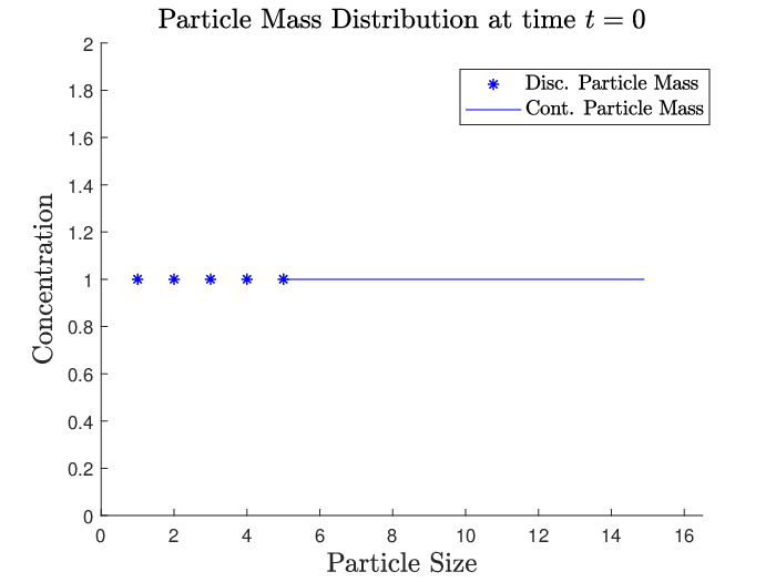
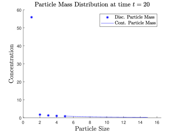
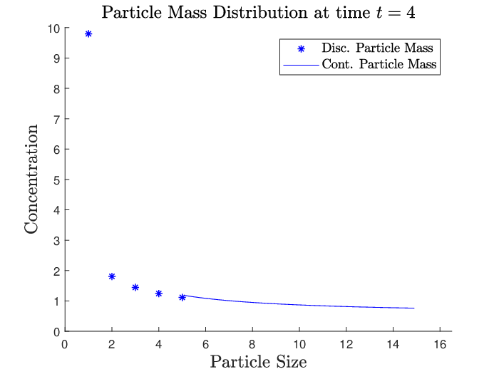
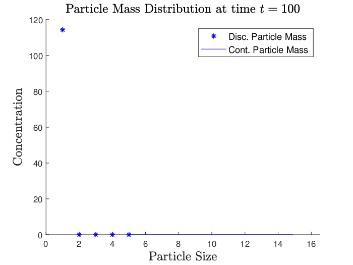
The above charts depict the behaviour one would expect given the physical nature of the model, with the mass becoming increasingly concentrated amongst the smaller sized particles. Additionally, the solution can be seen to remain nonnegative, as predicted by Lemma 6.1. However, to get a clearer picture of whether the issue of ‘shattering’ has been resolved we must examine the evolution of the total mass within the system.

Figure 2 details the evolution of the total mass (blue), along with the mass accounted for by the continuous regime (red), the total mass within the discrete regime (black) and the total mass accounted for by monomers (magenta).
As we would hope and as was predicted by Lemma 6.2, the total mass within the system remains constant, with a reduction in the continuous regime total mass being balanced by a gain in the total mass of the discrete regime, resulting from the fragmentation of larger continuous mass particles into smaller discrete mass particles. As time evolves, the mass accounted for by monomers grows to form an ever larger proportion of the total mass, until we reach a stage where they constitute the vast majority of the total mass and the system approaches an equilibrium.
7.3. Example Case 2 ( and )
In order to investigate the model behaviour and whether it fits with our physical intuition regarding the system, we vary the model parameters and observe the effect on the computed solutions. In this example we set and , which has the effect of increasing the fragmentation rate and changing the resulting size distribution for fragmentation events, to favour smaller particles. We would expect both of these changes to speed up the fragmentation process, and for equilibrium to be reached quicker than in the previous case. As before, we selected , with the same initial state (7.7). The final time was taken as , which we found to be sufficient for the system to reach a (near) equilibrium state and gave rise to the graphs in Figure 3.

As before, we see that the total mass (blue) is conserved with the loss from the continuous regime (red) being balanced by an increase in the discrete regime (black). However if we compare the model behaviour to that observed in Figure 2, we see that the process reaches an equilibrium state significantly quicker than in the previous case, as expected from an intuitive consideration of the model setup.
8. Conclusions
In this work we introduced a mixed discrete–continuous fragmentation model (1.1) and (1.2). Utilising the theory of operator semigroups we were able to prove that under certain restrictions on the fragmentation rate, there exists a unique, strong solution to our system within the setting of the appropriate Banach space. In turn, this enabled us to establish the existence of a unique classical solution to our equations. Finally, we showed that these solutions preserve nonnegativity and conserve mass, two properties we would expect from a physically relevant solution. We have illustrated the theoretical results by considering a specific example of such a mixed model, an example based upon existing models, which appear commonly in the literature of the field. The examples corroborated the analysis of the paper, with the solutions displaying the nonnegativity and mass conservation predicted.
Acknowledgments
This work was supported by the UK Engineering and Physical Sciences Research Council [EP/J500495/1 03].
References
- [1] M. Smoluchowski, Drei Vorträge über Diffusion, Brownsche Molekularbewegung und Koagulation von Kolloidteilchen, Physik. Z. 17 (1916) 557–585.
- [2] R. Ziff, Kinetics of polymerization, Journal of Statistical Physics 23 (2) (1980) 241–263.
- [3] P. Degond, J.-G. Liu, R. Pego, Coagulation–fragmentation model for animal group-size statistics, Journal of Nonlinear Science 27 (2) (2017) 379–424.
- [4] A. Johansen, F. Brauer, C. Dullemond, H. Klahr, A coagulation-fragmentation model for the turbulent growth and destruction of preplanetesimals 486 (2) (2008) 597–611.
- [5] E. McGrady, R. Ziff, Shattering transition in fragmentation, Phys. Rev. Lett. 58 (1987) 892–895.
- [6] J. Huang, X. Guo, B. Edwards, A. Levine, Cut-off model and exact general solutions for fragmentation with mass loss, J. Phys. A: Math. Gen. 29 (23) (1996) 7377–7388.
- [7] K. Engel, R. Nagel, One-Parameter Semigroups for Linear Evolution Equations, Springer, New York, 2000.
- [8] J. Banasiak, L. Arlotti, Perturbations of Positive Semigroups with Applications, Springer-Verlag, London, 2006.
- [9] J. Banasiak, On an extension of Kato–Voigt perturbation theorem for substochastic semigroups and its application, Taiwanese Journal of Mathematics 5 (1) (2001) 169–191.
- [10] W. Lamb, Existence and uniqueness results for the continuous coagulation and fragmentation equation, Math. Meth. Appl. Sci. 27 (2004) 703–721.
- [11] J. Banasiak, W. Lamb, On the application of substochastic semigroup theory to fragmentation models with mass loss, J. Math. Anal. Appl. 284 (2003) 9–30.
- [12] J. Banasiak, W. Lamb, Coagulation, fragmentation and growth processes in a size structured population, Discrete Contin. Dyn. Syst. Ser. B 11 (3) (2009) 563–585.
- [13] P. Blair, W. Lamb, I. Stewart, Coagulation and fragmentation with discrete mass loss, J. Math. Anal. Appl. 329 (2) (2007) 1285–1302.
- [14] A. McBride, A. Smith, W. Lamb, Strongly differentiable solutions of the discrete coagulation–fragmentation equation, Physica D: Nonlinear Phenomena 239 (15) (2010) 1436 – 1445.
- [15] L. Smith, W. Lamb, M. Langer, A. McBride, Discrete fragmentation with mass loss, Journal of Evolution Equations 12 (2012) 181–201.
- [16] R. Nagel, Towards a matrix theory for unbounded operator matrices, Math. Z. 201 (1989) 57–68.
- [17] J. Banasiak, Shattering and non-uniqueness in fragmentation models – an analytic approach, Physica D 222 (2006) 63–72”.
- [18] A. Pazy, Semigroups of Linear Operators and Applications to Partial Differential Equations, Springer, New York, 1983.
- [19] T. Kato, Perturbation Theory for Linear Operators, Springer-Verlag, Berlin, 1995.
- [20] A. Belleni-Morante, A. McBride, Applied Nonlinear Semigroups, Wiley, Chichester, 1998.
- [21] R. Simha, Kinetics of degradation and size distribution of long chain polymers, J. Appl. Phys. 12 (1941) 569.
- [22] R. Ziff, An explicit solution to a discrete fragmentation model, Journal of Physics A: Mathematical and General 25 (9) (1992) 2569.