Impact models of gravitational and electrostatic forces
Potential energies, atomic clocks, gravitational anomalies and redshift
Abstract
The far-reaching gravitational force is described by a heuristic impact model with hypothetical massless entities propagating at the speed of light in vacuum and transferring momentum and energy between massive bodies through interactions on a local basis. In the original publication [145], a spherical symmetric emission of secondary entities had been postulated. The potential energy problems in gravitationally and electrostatically bound two-body systems have been studied in the framework of this impact model of gravity and of a proposed impact model of the electrostatic force [146]. These studies have indicated that an anti-parallel emission of a secondary entity – now called graviton – with respect to the incoming one is more appropriate. This article is based on the latter choice and presents the modifications resulting from this change. The model has been applied to multiple interactions of gravitons in large mass conglomerations in several publications. They will be summarized here taking the modified interaction process into account. In addition, the speed of photons as a function of the gravitational potential are considered in this context together with the dependence of atomic clocks and the redshift on the gravitational potential.
wilhelm@mps.mpg.de00footnotetext: Department of Physics, Indian Institute of Technology (Banaras Hindu University), Varanasi-221005, India
bnd.app@iitbhu.ac.in
Last updated on August 24, 2026
Keywords Gravitation, secular mass increase, redshift, anomalies electrostatics, potential energies
PACS: 04.20.Cv, 04.25.-g, 04.50.Kd, 04.90.+e 41.20.Cv 98.62.Dm
I Introduction
Newton’s law of gravity gives the attraction between two spherical symmetric bodies A and B with masses and , a separation distance, (large compared to the sizes of the particles), and at rest in an inertial frame of reference. The force acting on B is
| (1) |
where is the constant of gravity11 1 This value and those of other constants are taken from CODATA 2014 [85]., is the unit vector of the radius vector with origin at A, and . The first term on the right-hand side represents the classical gravitational field of the mass .
In close analogy, Coulomb’s law yields the force of the electrostatic interaction between particles C with charge and D with charge :
| (2) |
where is the electric constant in vacuum. Here charges with opposite sign lead to attraction and with equal signs to repulsion.
| (3) |
is the classical electric field of a charge .
For two electrons, for instance, the ratio is
| (4) |
Newton’s law of gravitation yields a very good approximation of gravitational forces, unless effects treated in the General Theory of Relativity (GTR) [34] are of importance.
Nevertheless, the physical processes – in particular the potential
energies – of the gravitational
and the electrostatic fields are still a matter of debate:
Planck [98] wondered about the energy and momentum of the
electromagnetic field. A critique of the classical field theory by
Wheeler & Feynman [132] concluded that a theory of action at a distance,
originally proposed by Schwarzschild [114], avoids the direct notion of fields.
Lange [67, p. 231] calls the fact “remarkable” that the motion of a
closed system in response to external forces is determined by the same law as
its constituents. In this context, it should be recalled that von Laue [68]
considered radiation confined in a certain volume (,,Hohlraumstrahlung”) and
showed that the radiation contributed to the mass of the system according to
Einstein’s mass-energy equation, see Eq. (51).
In a discussion of energy-momentum conservation for gravitational fields,
Penrose [96, p. 468] finds even in closed systems “something a little
‘miraculous’ about how things all fit together, … ”; and
Carlip [20] wrote: “… after all, potential energy is a rather mysterious
quantity to begin with …”.
Related to the potential energy problem is the disagreement of Wolf et al. [149] and Müller et al. [86] on whether the frequency of an atomic clock – causing the gravitational redshift – is sensitive to the gravitational potential
| (5) |
or to the local gravity field .
These remarks and disputes motivated us to think about electrostatic and gravitational fields and the problems related to the potential energies.
II Gravitational and electrostatic interactions
If far-reaching fields have to be avoided, gravitational and electrostatic models come to mind similar to the emission of photons from a radiation source and their absorption or scattering somewhere else – thereby transferring energy and momentum with the speed of light, , in vacuum [99, 35, 21, 72].
A heuristic model of Newton’s law of gravitation has been proposed by Wilhelm et al. [145, Paper 1],– without far-reaching gravitational fields – involving hypothetical massless entities. Originally they had been called quadrupoles, but will be called gravitons now. In subsequent studies, conducted to test the model hypothesis, it became evident that the energy and momentum could not be conserved in a closed system without modifying the interaction process of the gravitons with massive bodies and massless particles, such as photons. The modification and the consequences in the context of the gravitational potential energy will be discussed in the following sections together with related topics.
The analogy between Newton’s and Coulomb’s laws suggest that in the latter case an impact model might be appropriate as well – with electric dipole entities transferring momentum and energy. This has been proposed in Paper 2 [146]. The equations governing the behaviour of gravitons and dipoles in the next sections are very similar in line with the similarity of Newton’s and Coulomb’s laws.
Both concepts are required for a description of the gravitational redshift in terms of physical processes in Sect. III.8.
II.1 Definitions of gravitons
Without a far-reaching gravitational field, the interactions have to be understood on a local basis with energy and momentum transfer by gravitons. This interpretation has several features in common with a theory based on gravitational shielding conceived by Nicolas Fatio de Duilleir [42] at the end of the seventeenth century. A French manuscript can be found in Bopp [16], and an outline in German has been provided by Zehe [153]. Related ideas by Le Sage have been discussed by Drude [26].
The gravitational case, in contrast to the electrostatic one, does not depend on polarized particles. Gravitons with an electric quadrupole configuration propagating with the speed of light will be postulated in the case of gravity. They are the obvious candidates as they have small interaction energies with positive and negative electric charges, and, in addition, can easily be constructed with a spin of , if indications to that effect are taken into account [130, cf.].
The vacuum is thought to be permeated by the gravitons that are, in the absence of near masses, isotropically distributed with (almost) no interaction among each other – even dipoles have no mean interaction energy in the classical theory [56, 57, see, e.g.]. The graviton distribution is assumed to be a nearly stable, possibly slowly varying quantity in space and time. It has a constant spatial number density
| (6) |
Constraints on the energy spectrum of the gravitons will be considered in later sections. At this stage we define a mean energy of
| (7) |
for a massless graviton with a momentum vector of .
II.2 Definitions of dipoles
A model for the electrostatic force can be obtained by introducing hypothetical electric dipoles propagating with the speed of light. The force is described by the action of dipole distributions on charged particles. The dipoles are transferring momentum and energy between charges through interactions on a local basis.
Apart from the requirement that the absolute values of the positive and negative charges must be equal, nothing is known, at this stage, about the values themselves, so charges of will be assumed, where might or might not be identical to the elementary charge .
The electric dipole moment is
| (8) |
parallel or antiparallel to the velocity vector , where is a unit vector pointing in a certain direction. This assumption is necessary in order to get attraction and repulsion of charges depending on their mutual polarities. In Sect. II.5 it will be shown that the value of the dipole moment is not critical in the context of our model. The dipoles have a mean energy
| (9) |
where represents the momentum of the dipoles. As a working hypothesis, it will first be assumed that is constant remote from gravitational centres with the same value for all dipoles of an isotropic distribution. The dipole distribution is assumed to be nearly stable in space and time with a spatial number density
| (10) |
but will be polarized near electric charges and affected by gravitational centres.
II.3 Virtual entities
As an important step, a formal way will be outlined of achieving the required momentum and energy transfers by discrete interactions. The idea is based on virtual gravitons or dipoles in analogy with other virtual particles [131, 152, 89, cf., e.g.].
II.3.1 Virtual gravitons
The virtual gravitons with energies of supplied by a central body with mass will have a certain lifetime and interact with “real” gravitons. In the literature, there are many different derivations of an energy-time relation [75, 4, 52, cf.]. Considerations of the spread of the frequencies of a limited wave-packet led Bohr [14] to an approximation for the indeterminacy of the energy that can be re-written as
| (11) |
with , the Planck constant. For propagating gravitons, the equation
| (12) |
is equivalent to the photon energy relation , where corresponds to , which can be considered as the wavelength of the hypothetical gravitons. Since there is experimental evidence that virtual photons (identified as evanescent electromagnetic modes) behave non-locally [74, 122], the virtual gravitons might also behave non-locally. Consequently, the absorption of a real graviton could occur momentarily by a recombination with an appropriate virtual one.
II.3.2 Virtual dipoles
We assume that a particle with charge is symmetrically emitting virtual dipoles with . The emission rate is proportional to its charge, and the orientation such that a repulsion exists between the charge and the dipoles. The symmetric creation and destruction of virtual dipoles is sketched in Fig. 1. The momentum balance is shown for the emission phase on the left and the absorption phase on the right side.

Virtual dipoles with energies of will have a certain lifetime and interact with real dipoles. The momentum and energy relations correspond to those of the gravitons:
| (13) |
The equation
| (14) |
is also equivalent to the photon energy relation for propagating dipoles, with corresponding to .
II.4 Newton’s law of gravity
The gravitons are absorbed by massive bodies from the background and subsequently emitted at rates determined by the mass of the body independent of its charge:
| (15) |
where is the gravitational absorption coefficient and the corresponding emission coefficient.
Spatially isolated particles at rest in an inertial system will be considered first. The sum of the absorption and emission rates is set equal to the intrinsic de Broglie frequency of the particle [18, 112, 113, 53, 50, 96, cf. Schrödinger’s Zitterbewegung; ]. Since the absorption and emission rates must be equal in Eq. (15), this gives an emission coefficient of
| (16) |
i.e. half the intrinsic de Broglie frequency, since two virtual gravitons
are involved in each absorption/emission process
(cf. Fig. 2). The absorption coefficient is constant,
because both and are constant.
For an electron, for instance, with a mass of
, the virtual graviton
production rate equals its de Broglie frequency
.
The energy absorption rate of an atomic particle with mass is
| (17) |
Larger masses are thought of as conglomeration of atomic particle.
The emission energy, in turn, is assumed to be reduced to
| (18) |
per graviton, where () is defined as the reduction parameter. This leads to an energy emission rate of
| (19) |
Without such an assumption the attractive gravitational force could not be emulated, even with some kind of shadow effect as in Fatio’s concept [16, cf.].

The reduction parameter and its relation to the attraction is discussed below. If the energy-mass conservation [30] is applied, its consequence is that the mass of matter increases with time at the expense of the background energy of the graviton distribution.
A spherically symmetric emission of the liberated gravitons had been assumed in Paper 1. Further studies summarized in Sects. III.1, III.6 and III.8 indicated that an anti-parallel emission with respect to the incoming graviton has to be assumed in order to avoid conflicts with energy and momentum conservation principles in closed systems. This important assumption can best be explained by referring to Fig. 2. The interaction is based on the combination of a virtual graviton with momentum ∗ and an incoming graviton with followed by the liberation of another virtual graviton in the opposite direction supplied with the excess energy . Regardless of the processes operating in the immediate environment of a massive body, it must attract the mass of the combined real and virtual gravitons, which will be at rest in the reference frame of the body. The excess energy is, therefore, reduced and so will be the liberation energy, as assumed in Eq. (18). The emission in Eq. (19) will give rise to a flux of gravitons with reduced energies in the environment of a body with mass . Its spatial density is
| (20) |
where the volume increase is
| (21) |
The radial emission is part of the background in Eq. (6), which has a larger number density than at most distances, , of interest. Note that the emission of the gravitons from does not change the number density or the total number of gravitons. For a certain , defined as the mass radius of , it has to be
| (22) |
because all gravitons of the background that come so close interact with the mass in some way. The same arguments apply to a mass and, in particular, to the electron mass, . Therefore
| (23) |
will be independent of the mass as long as the density of the background distribution is constant. The quantity is a kind of surface mass density. The equation shows that is determined by the electron mass radius, , for which estimates will be provided in Sects III.2 and III.3. From Eqs. (16), (22), and (23), it follows that
| (24) |
The flux of modified gravitons from will interact with a particle of mass and vice versa. The interaction rate in the static case can be found from Eqs. (15) and (20):
| (25) |
A calculation with anti-parallel emissions of the secondary gravitons shows that an interaction of a graviton with reduced momentum - provides together with its unmodified counterpart from the opposite sides. The resulting imbalance will be
| (26) |
if the quadratic terms in can be neglected for very small scenarios.
The imbalance will cause an attractive force that is responsible for the gravitational pull between bodies with masses and . By comparing the force expression in Eq. (26) with Newton’s law in Eq. (1), a relation between , , and can be established through the constant :
| (27) |
It can be seen that does not depend on the mass of a body. Since Eq. (18) allows stable processes over cosmological time scales only, if is very small, we assume in Fig. 3 that .
Note that the mass of a body and thus its intrinsic de Broglie frequency are not strictly constant in time, although the effect is only relevant for cosmological time scales, see lower panel of Fig. 3. In addition, multiple interactions will occur within large mass conglomerations (see Sects. III.4 to III.6), and can lead to deviations from Eqs. (1).
The graviton energy density remote from any masses will be
| (28) |
where the last term is obtained from Eq. (27) with the help of Eqs. (16) and (22) to (24).
What will be the consequences of the mass accretion required by the modified model? With Eqs. (17), (19) and (27), it follows that the relative mass accretion rate of a particle with mass will be
| (29) |
which implies an exponential growth according to
| (30) |
where is the initial value at and the linear approximation is valid for small . The accretion rate is
| (31) |
if the expression is evaluated in terms of recent parameters.

With these assumptions, the gravitational quantities are displayed in Fig. 3 in a wide parameter range (although the limits are set rather arbitrarily). The lower panel displays the time constant of the mass accretion. It indicates that a significant mass increase would be expected within the standard age of the Universe of the order of (with a Hubble constant of ) only for very small . Fahr & Heyl [40] have suggested that a decay of the vacuum energy density creates mass in an expanding Universe, and Fahr & Siewert [41] found a mass creation rate in accordance with Eq. (30).
The relative uncertainty of the present knowledge of the Rydberg constant
| (32) |
is , where
| (33) |
is Sommerfeld’s fine-structure constant. Since spectroscopic observations of the distant Universe with redshifts up to are compatible with modern data, it appears to be reasonable to set at least for s. Any variation of , caused by the linear dependence upon the electron mass, which has also been considered by Fahr [39], would then be below the detection limit for state-of-the-art methods.
II.5 Coulomb’s law
II.5.1 Electric fields and charged particles
Coulomb’s law in Eq. (2) gives the attractive or repulsive electrostatic force between two charged particles at rest in an inertial system. Together with the electric field in Eq. (3) it can be written as
| (36) |
The electric potential, , of a charge, , located at is
| (37) |
for . The corresponding electric field can thus be written as .
II.5.2 Dipole interactions
Note that the dipoles in the background distribution, cf. Eq. (10), have no mean interaction energy, even in the classical theory [57, see e. g.]. Whether this “background dipole radiation” and the “graviton radiation” are related to the dark matter (DM) and dark energy (DE) problems is of no concern here, but could be an interesting speculation.

A charge, , absorbs and emits dipoles at a rate
| (38) |
where and are the corresponding (dipole) emission and absorption coefficients.
From energy conservation it follows that absorption and emission rates of dipoles in Eq. (38) of a body with charge must be equal. The momentum conservation can, in general, be fulfilled by isotropic absorption and emission processes.
The interaction processes assumed between a positively charged body and dipoles is sketched in Fig. 4. A mass of the charge has explicitly been mentioned, because the massless dipole charges are not assumed to absorb and emit any dipoles themselves. The conservation of momentum could hardly be fulfilled in such a process. In Sect. III.8 we postulate, however, that gravitons interact with dipoles and thereby control their momentum and speed, subject to the condition that .
The assumptions as outlined will lead to a distribution of the emitted dipoles in the rest frame of an isolated charge, , with a spatial density of
| (39) |
where is given in Eq. (21). The radial emission is part of the background , which has a larger number density than at most distances, , of interest. Note that the emission of the dipoles from does not change the number density, , in the environment of the charge, but reverses the orientation of half of the dipoles affected.
The total number of dipoles will, of course, not be changed either. For a certain , defined as the charge radius of , it has to be
| (40) |
because all dipoles of the background that come so close interact with the charge in some way. The same arguments apply to a charge . Since cannot depend on either or , the quantity
| (41) |
must be independent of the charge, and can be considered as a kind of surface charge density, cf. ,,Flächenladung” of an electron defined by Abraham [1], that is the same for all charged particles. The equation shows that is determined by the electron charge radius, .
At this stage, this is a formal description awaiting further quantum electrodynamic studies in the near-field region of charges. It might, however, be instructive to provide a speculation for the dipole emission rate of a charge . The physical constants , , , and can be combined to give a dipole emission coefficient
| (42) |
as half the virtual dipole production rate and thus for a charge a rate
| (43) |
Note that dipole emission rate, in contrast to the assumptions in Fig. 5 of Paper 2, is fixed for a certain charge and does not depend on the particle mass.
| (44) |
During a direct interaction, the dipole A- (in Fig. 4 on the right side) combines together with an identical virtual dipole with an opposite velocity vector. This postulate is motivated by the fact that it provides the easiest way to eliminate the charges and yield (where is the momentum of the virtual dipole) as well as . The momentum balance is neutral and the excess energy, , is used to liberate a second virtual dipole B+, which has the required orientation. The charge had emitted two virtual dipoles with a momentum of , each, and a total momentum of was transferred to . The process can be described as a reflection of a dipole together with a reversal of the dipole momentum. The number of these direct interactions will be denoted by . The dipole of type A+ (on the left side) can exchange its momentum in an indirect interaction only on the far side of the charge with an identical virtual dipole during its absorption (or destruction) phase (cf. Fig. 1). The excess energy of is supplied to liberate a second virtual dipole B+. The momentum transfer to the charge is zero. This process just corresponds to a double charge exchange. Designating the number of interactions of the indirect type with , it is
| (45) |
with . Unless direct and indirect interactions are explicitly specified, both types are meant by the term “interaction”.
The virtual dipole emission rate in Fig. 4 has to be
| (46) |
i.e., the virtual dipole emission rate equals the sum of the real absorption and emission rates. The interaction model described results in a mean momentum transfer per interaction of without involving a macroscopic electrostatic field.
A quantitative evaluation gives the force acting on a test particle with charge, , at a distance, , from another particle with charge . This results from the absorption of dipoles not only from the background, but also from the distribution emitted from according to Eq. (39) under the assumption of a constant absorption coefficient, in Eq. (38). The rate of interchanges between these charges then is
| (47) |
which confirms the reciprocal relationship between and . The equation, also very similar to Eq. (25), does not contain an explicit value for . It is important to realize that all interchange events between pairs of charged particles are either direct or indirect depending on their polarities and transfer a momentum of or zero.
The external electrostatic potential of a spherically symmetric body C with charge is given in Eq. (37). Since the electrostatic forces between the charged particles C and D are typically many orders of magnitude larger than the gravitational forces, we only take the electrostatic effects into account in this section and neglect the gravitational interaction.
In order to have a well-defined configuration for our discussion, we will assume that body C with mass has a positive charge and is positioned at a distance beneath body D (mass ) with either a charge in Fig. 5 or in Fig. 6. Only the processes near the body D are shown in detail.
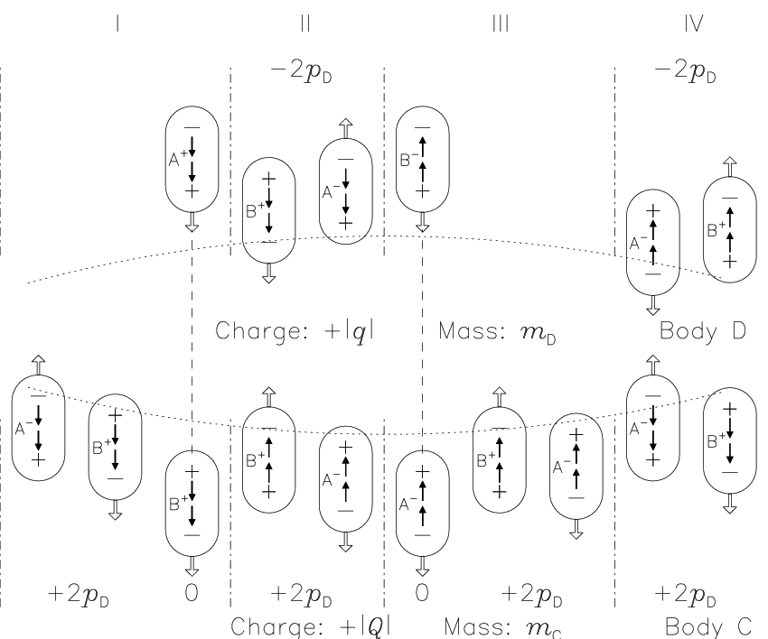

The interaction rates of dipoles with bodies C and D in Eq. (47) (the same for both bodies even if ) and the momentum transfers indicated in Figs. 5 and 6, respectively, lead to a norm of the momentum change rate for bodies C and D of
| (48) |
Together with
| (49) |
this leads, depending on the signs of the charges and , to a repulsive or an attractive electrostatic force between C and D in accordance with Coulomb’s law in Eq. (2).
Important questions are related to the energy and momentum of the dipoles and, even more, to their energy density in space. Eqs. (9), (40), (41), and (44) together with Eq. (49) allow the energy density to be expressed by
| (50) |
This quantity is independent of the dipole energy. It takes into account all dipoles (whether their distribution is chaotic or not). Should the energy density vary in space and / or time, the surface charge density, , must vary as well.
If we assume that the electron charge radius in Eq. (41) equals the classical electron radius 2.82 fm, very high energy densities of , compared to the cosmic dark energy estimate, follow from Eq. (50). The dipole density in Eq. (40) is also very high with leading to a dipole energy of . If, on the other hand, we identify the dipole distribution with DM with an estimated energy density of and require that the dipole energy density corresponds to this value, then rather unlikely values follow for , and .
III Applications of impact models
The detection of gravitons and dipoles with the expected properties would, of course, be the best verification of the proposed models. Laking this, indirect support can be found through the application of the models with a view to describe physical processes successfully for specific situations.
III.1 Potential energies
III.1.1 Gravitational potential energy
As mentioned in Sect. I the study of the potential energy problem [140] had been motivated by the remark that the potential energy is rather mysterious [20]22 2 In this context it is of interest that Brillouin [17] discussed this problem in relation to electrostatic potential energy.. It led to the identification of the “source region” of the potential energy for the special case of a system with two masses and subject to the condition . An attempt to generalize the study without this condition required either violations of the energy conservation principle as formulated by von Laue [70] for a closed system, or a reconsideration of an assumption we made concerning the gravitational interaction process in Paper 1. The change necessary to comply with the energy conservation principle has been discussed in Sect. II.4. A generalization of the potential energy concept for a system of two spherically symmetric bodies A and B with masses and without the above condition could then be formulated [141].
We will again exclude any further energy contributions, such as rotational or thermal energies, and make use of the fact that the external gravitational potential of a spherically symmetric body of mass and radius in Eq. (5) is that of a corresponding point mass at the centre.
The energy and the momentum of a free particle with mass moving with a velocity relative to an inertial reference system are related by
| (51) |
where is the momentum vector
| (52) |
[29, 30]. For an entity in vacuum with no rest mass (), such as a photon [28, 72, 92, cf.], the energy-momentum relation in Eq. (51) reduces to
| (53) |
We now assume that two spherically symmetric bodies A and B with masses and , respectively, are placed in space remote from other gravitational centres at a distance of reckoned from the position of A. Initially both bodies are at rest with respect to an inertial reference frame represented by the centre of gravity of both bodies. The total energy of the system then is with Eq. (51) for the rest energies and with Eq. (5) for the potential energy
| (54) |
The evolution of the system during the approach of A and B from to can be described in classical mechanics. According to Eq. (48), the attractive force between the bodies during the approach is approximately constant for , resulting in accelerations of and , respectively. Since the duration of the free fall of both bodies is the same, the approach of A and B can be formulated as
| (55) |
showing that , i.e, the centre of gravity stays at rest. Multiplication of Eq. (55) by gives the corresponding kinetic energy equation
| (56) |
The kinetic energies33 3 Eqs. (51) and (52) together with [30] and yield the relativistic kinetic energy of a massive body: . The evaluations for and agree in very good approximation with Eq. (56) for small and . and should, of course, be the difference of the potential energy in Eq. (54) at distances of and . We find indeed with Newton’s law in Eq. (1)
| (57) |
We may now ask the question, whether the impact model can provide an answer to the potential energy “mystery” in a closed system. Since the model implies a secular increase of mass of all bodies, it obviously violates a closed-system assumption. The increase is, however, only significant over cosmological time scales, and we can neglect its consequences in this context. A free single body will, therefore, still be considered as a closed system with constant mass. In a two-body system both masses and will be constant in such an approximation, but now there are gravitons interacting with both masses.
The number of gravitons travelling at any instant of time from one mass to the other can be calculated from the interaction rate in Eq. (25) multiplied by the travel time :
| (58) |
The same number is moving in the opposite direction. The energy deficiency of the interacting gravitons with respect to the corresponding background then is together with Eqs. (18) and (27) for each body
| (59) |
The last term shows – with reference to Eq. (57) – that the energy deficiency equals half the potential energy of body A at a distance from body B and vice versa.
We now apply Eq. (59) and calculate the difference of the energy deficiencies for separations of and for interacting gravitons travelling in both directions and get
| (60) |
Consequently, the difference of the potential energies between and in Eq. (57) is balanced by the difference of the total energy deficiencies.
The physical processes involved can be described as follows:
- 1.
The number of gravitons on their way for a separation of is smaller than that for , because the interaction rate depends on according to Eq. (48), whereas the travel time is proportional to .
- 2.
A decrease of to during the approach of A and B increases the number of gravitons with reduced energy.
- 3.
The energies liberated by energy reductions are available as potential energy and are converted into kinetic energies of the bodies A and B.
- 4.
With Eqs. (51) and (52) and the approximations in Footnote 3, it follows that the sum of the kinetic energies and , the masses A and B plus the total energy deficiencies of the interacting gravitons can indeed be considered to be a closed system as defined by von Laue [70].
III.1.2 Electrostatic potential energy
In this section we will discuss the electrostatic aspects of the potential energy.
The energy density of an electric field outside of charges is given by
| (61) |
[54, 57, cf., e.g.]. Applying Eq. (61) to a plane plate capacitor with an area , a plate separation and charges on the plates, the energy stored in the field of the capacitor turns out to be
| (62) |
With a potential difference and a charge of (incrementally increased to these values), the potential energy of at is
| (63) |
The question as to where the energy is actually stored, Hund [54] answered by showing that both concepts implied by Eqs. (62) and (63) are equivalent.
Can the impact model provide an answer for the electrostatic potential energy in a closed system, where dipoles are interacting with two charged bodies? The number of reversed dipoles travelling at any instant of time from a charge to in Figs. 5 and 6 can be calculated from the interaction rate in Eq. (47) multiplied by a travel time :
| (64) |
The same number of dipoles is moving in the opposite direction from to . From Eqs. (9), (49) and (64), we can determine the total energy of the reversed dipoles:
| (65) |
It is equal to the absolute value of the electrostatic potential energy of a charge at the electric potential in Eq. (37) of a charge .
The evolution of the system is similar to that of the gravitational case in Sect. III.1.1, however, attraction and repulsion have to be considered during the approach or separation of bodies C and D. The initial distance between C and D be , when both bodies are assumed to be at rest, and changes to by the repulsive or attractive force between the charges given by Coulomb’s law in Eq. (2) The force is approximately constant for causing accelerations of and , respectively. Since the duration of the motions of both bodies is the same, the separation (upper sign) or approach (lower sign) of C and D can be formulated as follows:
| (66) |
Comparing the second term of the equation with the last one, it can be seen that , i.e. the centre of gravity stays at rest. Multiplication of Eq. (66) by gives a good estimate of the corresponding kinetic energy:
| (67) |
where and are the speeds of the bodies, when the distances between C and D are attained. The sum of the kinetic energies and must, of course, be equal to the difference of the electrostatic potential energy at distances of and :
| (68) |
The variations of the number of dipoles in Eqs. (58) and (65) during the separation or approach of bodies C and D from to are
| (69) |
The number of reversed dipoles thus decreases during the separation of C and D in Fig. 5. The corresponding energy variation with positive is, cf. Eq. (65):
| (70) |
The energy of the reversed dipoles thus decreases by the amount that fuels the kinetic energy in Eq. (67).
In the opposite case with negative and attraction, it can be seen from Fig. 6 that the increased number of reversed dipoles is actually leaving the system without momentum exchange and is lost. The momentum difference, therefore, is again negative
| (71) |
and so is the energy of the reversed dipoles confined in the system:
| (72) |
The electrostatically bound two-body system thus is a closed system in the sense defined by von Laue [70], slowly evolving in time during the movements of the bodies C and D. The potential energy converted into kinetic energy stems from the modified dipole distributions.
III.2 Pioneer anomaly
Anomalous frequency shifts of the Doppler radio-tracking signals were detected for both Pioneer spacecraft [7]. The observations of Pioneer 10 (launched on 2 March 1972) published by the Pioneer Team will be considered during the time interval, , between 3 January 1987 and 22 July 1998 (), while the spacecraft was at heliocentric distances between ua and ua. The Pioneer team took into account all known contributions in calculating a model frequency, , which was based on a constant clock frequency at the terrestrial control stations. Observations at times then indicated a nearly uniform increase of the observed frequency shift with respect to the expected one of
| (73) |
with [126, cf.].
The observations of the anomalous frequency shifts could, in principle, be interpreted as a deceleration of the heliocentric spacecraft velocity by
| (74) |
However, no unknown sunward-directed force could be identified [55, cf.]. Alternatively, a clock acceleration at the ground stations of
| (75) |
could explain the anomaly. A true trajectory anomaly together with an unknown systematic spacecraft effect was considered to be the most likely interpretation by Anderson et al. [8]. Although Turyshev et.al [127] later concluded that thermal recoil forces of the spacecraft caused the anomaly of Pioneer 10, the discussion in the literature continued.
Assuming an atomic clock acceleration, a constant reference frequency for the calculation of is not appropriate [134, cf.]. Consequently the equation
| (76) |
equivalent to Eq. (73), has to be modified with
| (77) |
and
| (78) |
to
| (79) |
The gravitationally impact model in Sect. II.4 leads to a secular mass increase of massive particles in Eq. (30). Consequently the Rydberg constant in Eq. (32) would increase in a linear approximation with the electron mass according to
| (80) |
resulting in frequency increases of atomic clocks with time. They give rise to the clock acceleration in Eq. (77), if we assume . The most likely values of in Fig. 3 range from to 2.82 fm, the classical electron radius, corresponding with Eq. (31) to , the Hubble constant, and . Within the uncertainty margins the high value agrees with in Eq. (75) and would quantitatively account for the Pioneer frequency shift.
Should the anomaly be much less pronounced, because thermal recoil forces decelerate the spacecraft, the range of in Fig. 3 could thus accommodate smaller values of as well.
III.3 Sun-Earth distance increase
A secular increase of the mean Sun-Earth distance with a rate of per century had been reported using many planetary observations between 1971 and 2003 [61]. Neither the influence of cosmic expansion nor a time-dependent gravitational constant seem to provide an explanation [65].
As our impact model summarized in Sect. II.4 leads to a secular mass increase according to Eq. (30) of all massive bodies fuelled by a decrease in energy of background flux of gravitons, it allowed us to formulate a quantitative understanding of the effect within the parameter range of the model [136].
The value of the astronomical unit is now defined as (exact) by the International Astronomical Union (IAU) and the Bureau International des Poids et Mesure [19]. The mean Sun-Earth distance is known with a standard uncertainty of (3 to 6) m for [97, 6, 47].
Considering this uncertainty, the measurement of a change rate of
| (81) |
is difficult, but feasible as relative determination. A circular orbit approximation had been considered, because the mean value of is of interest:
| (82) |
following from Eq. (1) and the centrifugal force with
, the tangential orbital velocity of the Earth, where
the heliocentric gravitational constant is
(IAU) and thus
the mass of the Sun
.
We now consider Eq. (82) not only for , but also at assuming constant as well as constant . The latter assumption is justified by the fact that any uniformly moving particle does not experience a deceleration. It implies an increase of the momentum together with the mass accumulation of the Earth. The apparent violation of the momentum conversation principle can be resolved by considering the accompanying momentum changes of the graviton distribution. A detailed discussion of this aspect is given in Sect. 3 of Paper 1.
III.4 Secular perihelion advances in the solar system
Multiple application of the interaction process described in Sect. II.4 can produce gravitons with reduction parameters greater than in large mass conglomerations – within the Sun in this section. The proportionality of the linear term in the binomial theorem with the exponent in
| (87) |
suggests that a linear superposition of the effects of multiple interactions will be a good approximation, if is not too large. Energy reductions according to Eq. (18) are therefore not lost, as claimed by Drude [26], but they are redistributed to other emission locations within the Sun. This has two consequences: (1) The total energy reduction is still dependent on the solar mass, and (2) since emissions from matter closer to the surface of the Sun in the direction of an orbiting object is more likely to escape into space than gravitons from other locations, the effective gravitational centre should be displaced from the centre of the Sun towards that object.
Using published data on the secular perihelion advances of the inner planets Mercury, Venus, Earth and Mars of the solar system and the asteroid Icarus, we found that the effective gravitational centre is displaced from the centre of the Sun by approximately [138]. Since an analytical derivation of this value from the mass distribution of the Sun was beyond the scope of the study, future investigations need to show that the modified process with directed secondary graviton emission can quantitatively account for such a displacement.
III.5 Planetary flyby anomalies
III.5.1 Earth flybys
Several Earth flyby manoeuvres indicated anomalous accelerations and decelerations and led to many investigations without reaching a solution of the problem, see recent reviews by Anderson et al. [9] and Nieto & Anderson [88]. Since there is general agreement that the anomaly is only significant near perigee, we discuss here the seven passages at altitudes below 2000 km listed in Table 1 of Acedo [2, note the wrong dates]. Three of them (Galileo I, NEAR and Rosetta) we have studied assuming the gravitational impact model of Sect. II.4 and multiple interactions [142]. As in Sect. III.4, the multiple interactions result in a deviation of the effective gravitational centre from the geometric centre. We obtained for Galileo, NEAR and Rosetta , respectively. The study had been conducted assuming a spherically symmetric emission of liberated gravitons mentioned in Sect. II.4.
With the assumption of an anti-parallel emission, we have repeated the analysis and found for all spacecraft, provided the origin of is shifted by approximately in the direction of the perigee of Galileo I, for NEAR, and for Rosetta. Moreover, it was possible to model the decelerations of Galileo II on 8 December 1992 with a shift of ; of Cassini on 18 August 1999 with and the null result for Juno on 9 October 2013 with .
An origin offset of opposite to the Cassini perigee could to a first approximation achieve all apparent shifts taking the geographic coordinates of the various flybys into account. A detailed study would have to consider in addition the Earth gravitational model.
III.5.2 Juno Jupiter flybys
Juno was inserted into an elliptical orbit around Jupiter on 4 July 2016 with an orbital period of 53.5 days. Acedo et al. [3] studied the first and the third orbit with a periapsis of “4200 km over the planet top clouds”. “A significant radial component was found and this decays with the distance to the center of Jupiter as expected from an unknown physical interaction. … The anomaly shows an asymmetry among the incoming and outgoing branches of the trajectory … .” The radial component is shown in their Figure 6 between min around perijove for the first and third Juno flyby. The peak anomalous outward accelerations shown are in both cases: at min and at min.
We applied the multiple-interaction concept of the previous Sects. III.4 and III.5.1, and found that offsets of (8 to 27) km of the gravitational from the geometric centre are required to model the acceleration in Fig. 7, which is in good agreement with the observations during the Juno Jupiter flybys. The variation of could be modelled by an ellipsoidal displacement of the gravitational centre offset in the direction of a flyby position near min.

III.6 Rotation velocities of spiral galaxies
The rotation velocities of spiral galaxies are difficult to reconcile with Keplerian motions, if only the gravitational effects of the visible matter is taken into account [106, 107, e.g.]. Dark matter had been proposed by Oort [94] and Zwicky [154] in order to understand several velocity anomalies in galaxies and clusters of galaxies. A MOdification of the Newtonian Dynamics (MOND) has been introduced by Milgrom [82] that assumes a modified gravitational interaction at low acceleration levels.
The impact model of gravitation in Sect. II.4 is applied to the radial acceleration of disk galaxies [144]. The flat velocity curves of NGC 7814, NGC 6503 and M 33 are obtained without the need to postulate any dark matter contribution. The concept explained below provides a physical process that relates the fit parameter of the acceleration scale defined by McGaugh et al. [78] to the mean free path length of gravitons in the disks of galaxies. It may also provide an explanation for MOND.
McGaugh [77] has observed a fine balance between baryonic and dark mass in spiral galaxies that may point to new physics for DM or a modification of gravity. Fraternali et al. [44] have also concluded that either the baryons dominate the DM or the DM is closely coupled with the luminous component. Salucci & Turini [109] have suggested that there is a profound interconnection between the dark and the stellar components in galaxies.
The large baryonic masses in galaxies will cause multiple interactions of gravitons with matter if their propagation direction is within the disk. For each interaction the energy loss of the gravitons is assumed to be (for details see Sect. 2.3 of Paper 1). The important point is that the multiple interactions occur only in the galactic plane and not for inclined directions. An interaction model is designed indicating that an amplification factor of approximately two can be achieved by six successive interactions. An amplification occurs for four or more interactions. The process works, of course, along each diameter of the disk and leads to a two-dimensional distribution of reduced gravitons.
The multiple interactions do not increase the total reduction of graviton energy, because the number of interactions is determined by the (baryonic) mass of the gravitational centre according to Paper 1. A galaxy with enhanced gravitational acceleration in two dimensions defined by the galactic plane, will, therefore, have a reduced acceleration in directions inclined to this plane.
III.7 Light deflection and Shapiro delay
The deflection of light near gravitational centres is of fundamental importance. For a beam passing close to the Sun Soldner [119] and Einstein [32] obtained a deflection angle of under the assumption that radiation would be affected in the same way as matter. Twice this value was then derived in the framework of the GTR [34]44 4 It is of interest in the context of this paper that Einstein employed Huygens’ Principle in his calculation of the deflection., and later by Schiff [110] using the equivalence principle and STR. The high value was confirmed during the total solar eclipse in 1919 for the first time [27]. This and later observations have been summarized by Mikhailov [81] and combined to a mean value of approximately 2′′.
The deflection of has also been considered in the context of the gravitational impact model summarized in Sect. II.4. As a secular mass increase of matter was a consequence of the this model, the question arises of how the interaction of gravitons with photons can be understood, since the photon mass is in all likelihood zero.55 5 A zero mass of photons follows from the STR and a speed of light in vacuum constant for all frequencies. Einstein [28] used ,,Lichtquant” for a quantum of electromagnetic radiation; the term “photon” was introduced by Lewis [72]. With various methods the photon mass could be constrained to [45, 5] or even to [150]. An initial attempt at solving that problem has been made in Wilhelm & Dwivedi [135] by assuming that a photon stimulates an interaction with a rate equal to its frequency . It is summarized here under the assumption of an anti-parallel re-emission, both for massive particles and photons.
A physical process will then be outlined that provides information on the gravitational potential at the site of a photon emission [143]. This aspect had not been covered in our earlier paper on the gravitational redshift [137].
Interactions between massive bodies have been treated in Paper 1 with an absorption rate of half the intrinsic de Broglie frequency of a mass, because two virtual gravitons have to be emitted for one interaction. The momentum transfer to a photon will thus be twice as high as to a massive body with a mass equivalent to .
We then apply the momentum conservation principle to photon-graviton pairs in the same way as to photons [66, cf.] and can write after a reflection of
| (88) |
with .
We assume, applying Eq. (88) with , that under the influence of a gravitational centre relevant interactions occur on opposite sides of a photon with and transferring a net momentum of . Note, in this context, that the Doppler effect can only operate for interactions of photons with massive bodies [43, 120, cf.]. Consequently, there will be no energy change of the photon, because both gravitons are reflected with constant energies under these conditions, and we can write for a pair of interactions
| (89) |
where is the photon momentum after the events. If and a component of are pointing in the same direction, it is , the speed is reduced; an antiparallel direction leads to . Note that this could, however, not result in , because can only be attained in a region with an isotropic distribution of gravitons with a momentum of , i.e. with a gravitational potential .
The momentum of a photon radially approaching a gravitational centre will be treated in line with Eq. (6) of Paper 2 for massive bodies, however, with twice the interactionrate for photons. Since we know from observations that the deflection of light near the Sun is very small, the momentum variation caused by the weak and static gravitational interaction is also very small. The momentum change rate of the photon can then be approximated by
| (90) |
where is the distance of the photon from the centre, and the position vector of the photon is with a unit vector . The small deflection angle also allows an approximation of the actual path by a straight line along an axis: . The normalized momentum variation along the trajectory then is
| (91) |
The corresponding component perpendicular to the trajectory is
| (92) |
where is the impact parameter of the trajectory. Integration of Eq. (91) over from to yields
| (93) |
If we apply Eq. (89) to a photon approaching the Sun along the axis starting from infinity with , and considering that the component in Eq. (91) is much smaller than the x component in Eq. (92) for , the photon speed as a function of can be determined from
| (94) |
Division by then gives with Eq. (93)
| (95) |
as a good approximation of the inverse gravitational index of refraction along the axis. The same index has been obtained albeit with different arguments, e.g. by Boonserm et al. [15], Ye & Lin [151]. The resulting speed of light is in agreement with evaluations by Schiff [110], for a radial propagation66 6 Einstein [33] states explicitly that the speed at a certain location is not dependent on the direction of the propagation. in a central gravitational field, and Okun [91] — calculated on the basis of the standard Schwarzschild metric. A decrease of the speed of light near the Sun, consistent with Eq. (95), is not only supported by the predicted and subsequently observed Shapiro delay [116, 105, 117, 60, 10, 63], but also indirectly by the deflection of light [27].
The deflection of light by gravitational centres according to the GTR [34] and its observational detection by Dyson et al. [27] leave no doubt that a photon is deflected by a factor of two more than expected relative to a corresponding massive particle. Since in our concept the interaction rate between photons and gravitons is twice as high as for massive particles of the same total energy, the reflection of a graviton from a photon with a momentum of must also be anti-parallel to the incoming one, i.e. a momentum of will be transferred. Otherwise the correct deflection angle for photons cannot be obtained. This modified interaction process has one further important advantage: the reflected graviton can interact with the deflecting gravitational centre and – through the process outlined in the paragraph just before Eq. (48) – transfers , in compliance with the momentum conservation principle. In the old scheme, the violation of this principle had no observational consequences, because of the extremely large masses of relevant gravitational centres, but the adherence to both the momentum and energy conservation principles is very encouraging and clearly favours the new concept.
Basically the same arguments are relevant for the longitudinal interaction between photons and gravitons. The momentum transfer per interaction will be doubled, but the gravitational absorption coefficient will be reduced by a factor of two. Together with an increased graviton density, all quantities and results are the same as before. However, a detailed analysis shows that the momentum conservation principle is now also adhered to.
III.8 Gravitational redshift
The gravitational potential at a distance from a spherical body with mass is constraint in the weak-field approximation for non-relativistic cases [66, cf.] by
| (96) |
A definition of a reference potential in line with this formulation is for .
The study of the gravitational redshift, predicted for solar radiation by Einstein [31], is still an important subject in modern physics and astrophysics [59, 87, 64, 95, 125, e.g.]. This can be exemplified by two conflicting statements. Wolf et al. [149] write: “The clock frequency is sensitive to the gravitational potential and not to the local gravity field .” Whereas it is claimed by Müller et al. [86]: “We first note that no experiment is sensitive to the absolute potential .”
Support for the first alternative can be found in many publications [31, 70, 110, 147, 93, 118, e.g.], but it is, indeed, not obvious how an atom can locally sense the gravitational potential . Experiments on Earth, in space and in the Sun-Earth system [101, 62, 102, 128, 73, 124, cf., e.g.] have, however, quantitatively confirmed in the static weak field approximation a relative frequency shift of
| (97) |
where is the frequency of the radiation emitted by a certain transition at and the observed frequency there, if the emission caused by the same transition had occurred at a potential .
Since Einstein discussed the gravitational redshift and published conflicting statements regarding this effect, the confusion could still not be cleared up consistently [76, 121, cf., e.g.]. In most of his publications Einstein defined clocks as atomic clocks. Initially he assumed that the oscillation of an atom corresponding to a spectral line might be an intra-atomic process, the frequency of which would be determined by the atom alone [31, 32]. Scott [115] also felt that the equivalence principle and the notion of an ideal clock running independently of acceleration suggest that such clocks are unaffected by gravity. Einstein [34] later concluded that clocks would slow down near gravitational centres thus causing a redshift.
The question whether the gravitational redshift is caused by the emission process (Case a) or during the transmission phase (Case b) is nevertheless still a matter of recent debates. Proponents of (a) are, e.g.: Møller [84], Cranshaw et al. [22], Schiff [110], Ohanian [90], Okun et al. [93] and of (b): Hay et al. [48], Straumann [123], Randall [104], Will [148].
It is surprising that the same team of experimenters, albeit with different first authors (Cranshaw et al. and Hay et al.) published different views on the process of the Pound–Rebka–Experiment. Pound & Snider [102] and Pound [100] pointed out that this experiment could not distinguish between the two options, because the invariance of the velocity of the radiation had not been demonstrated.
Einstein [35] emphasized that for an elementary emission process not only the energy exchange, but also the momentum transfer is of importance [99, 1, 43, see also]. Taking these considerations into account, we formulated a photon emission process at a gravitational potential [137] assuming that:
- (1)
The atom cannot sense the potential , in line with the original proposal by Einstein [31], Einstein [32], and initially emits the same energy at and .
- (2)
It also cannot directly sense the speed of light at the location with a potential . The initial momentum thus is .
- (3)
As the local speed of light is, however, , a photon having an energy of and a momentum is not able to propagate. The necessary adjustments of the photon energy and momentum as well as the corresponding atomic quantities then lead in the interaction region to a redshift consistent with and observations.
As outlined in Sect. III.7, there is general agreement in the literature that the local speed of light is
| (98) |
in line with Eq. (95) in Sect. III.7. It has, however, to be noted that the speed was obtained for a photon propagating from to , and, therefore, the physical process which controls the speed of newly emitted photons at a gravitational potential is not yet established.
An attempt to do that will be made by assuming an aether model. Before we suggest a specific aether model, a few statements on the aether concept in general should be mentioned. Following Michelson & Morley [79] famous experiment, Einstein [29], Einstein [31] concluded that the concept of a light aether as carrier of the electric and magnetic forces is not consistent with the STR. In response to critical remarks by Wiechert [133], cf. Schröder [111] for Wiechert’s support of the aether, von Laue [69] wrote that the existence of an aether is not a physical, but a philosophical problem, but later differentiated between the physical world and its mathematical formulation. A four-dimensional ‘world’ is only a valuable mathematical trick; deeper insight, which some people want to see behind it, is not involved [71].
In contrast to his earlier statements, Einstein said at the end of a speech in Leiden that according to the GTR a space without aether cannot be conceived [36]; and even more detailed: Thus one could instead of talking about ‘aether’ as well discuss the ‘physical properties of space’. In theoretical physics we cannot do without aether, i.e., a continuum endowed with physical properties [37]. Michelson et al. [80] confessed at a meeting in Pasadena in the presence of H.A. Lorentz that he clings a little to the aether; and Dirac [25] wrote in a letter to Nature that there are good reasons for postulating an æther.
In Paper 2 we proposed an impact model for the electrostatic force based on massless dipoles. The vacuum is thought to be permeated by these dipoles that are, in the absence of electromagnetic or gravitational disturbances, oriented and directed randomly propagating along their dipole axis with a speed of . There is little or no interaction among them. We suggest to identify the dipole distribution postulated in Sect. II.5 with an aether. Einstein’s aether mentioned above may, however, be more related to the gravitational interactions [46, cf.]. In this case, we have to consider the graviton distribution as another component of the aether.
If we assume that an individual dipole interacts with gravitons in the same way as photons, see Eq. (89), according to
| (99) |
where and refer to the energy and momentum of a dipole. The condition , cf. Eq. (88), is fulfilled in the range from for all .
We can then modify Eqs. (90) to (94) by changing to D and find that Eqs. (95) and (98) are also valid for dipoles with a speed of for .
Considering that many suggestions have been made to describe photons as solitons [24, 129, 58, 83, 12, 13, e.g.], we also propose that a photon is a soliton propagating in the dipole aether with a speed of , cf. Eq. (98), controlled by the dipoles moving in the direction of propagation of the photon. The dipole distribution thus determines the gravitational index of refraction, cf. Eq. (95), and consequently the speed of light at the potential . This solves the problem formulated in relation to Eq. (98) and might be relevant for other phenomena, such as gravitational lensing and the cosmological redshift [38, cf., e.g.]. Should the speculation in Sect. II.5.2 be taken seriously that the dipole distribution corresponds to DM, it has to be much more evenly distributed than previously thought [51]. The light deflection would then be caused by gravitationally induced index of refracion variations.
IV Discussion and conclusions
With Newton’s law of gravitation as starting point, the ideas presented in Sect. II.4 allow an understanding of far-reaching gravitational force between massive particles as local interactions of hypothetical massless gravitons travelling with the speed of light in vacuum. The gravitational attraction leads to a general mass accretion of massive particles with time, fuelled by a decrease of the graviton energy density in space. The physical processes during the conversion of gravitational potential energy into kinetic energy have been described for two bodies with masses and and the source of the potential energy could be identified in Sect. III.1.1. In order to avoid conflicts with energy and momentum conservation, we had to modify a detail of the interaction process in Eq. (26), i.e., assume an anti-parallel of the secondary graviton with respect to the incoming one.
Multiple interactions of gravitons leading to shifts of the effective gravitational centre of a massive body from the “centre of gravity” are treated in Sects. III.4 to III.6 taking the modified concept into account. The interaction of gravitons with photons in Sect. III.7 had to be modified as well, but the modification did not change the results, with the exception that now both the energy and momentum conservation principles are fulfilled.
Our main aim in Sect. III.8 was to identify a physical process that leads to a speed of photons controlled by the gravitational potential . This could be achieved by postulating an aether model with moving dipoles, in which a gravitational index of refraction regulates the emission and propagation of photons as required by energy and momentum conservation principles. The emission process thus follows Steps (1) to (3) in Sect. III.8, where the local speed of light is given by the gravitational index of refraction . In this sense, the statement that an atom cannot detect the potential by Müller et al. [86] is correct; the local gravity field , however, is not controlling the emission process.
A photon will be emitted by an atom with appropriate energy and momentum values, because the local speed of light requires an adjustment of the momentum. This occurs in the interaction region between the atom and its environment as outlined in Step (3).
In the framework of a recently proposed electrostatic impact model in Paper 2, the physical processes related to the variation of the electrostatic potential energy of two charged bodies have been described and the “source region” of the potential energy in such a system could be identified and is summarized in Sect. III.1.2.
Sotiriou et al. [121] made a statement in the context of gravitational theories in ‘A no-progress report’: ‘[…] it is not only the mathematical formalism associated with a theory that is important, but the theory must also include a set of rules to interpret physically the mathematical laws’. With this goal in mind we have presented our ideas on the gravitational and electrostatic interactions.
Acknowledgements This research has made extensive use of the Smithsonian Astrophysical Observatory (SAO)/National Aeronautics and Space Administration (NASA) Astrophysics Data System (ADS). Administrative support has been provided by the Max-Planck-Institute for Solar System Research in Göttingen, Germany, and the Indian Institute of Technology (Banaras Hindu University) in Varanasi, India.
References
- [1] Abraham, M., 1902, Prinzipien der Dynamik des Elektrons. Ann. Phys. (Leipzig), 315, 105
- [2] Acedo, L., 2017, The flyby anomaly: a multivariate analysis approach, Astrophysics and Space Science, 362, id.42
- [3] Acedo, L., Piqueras, P., & Moraflo, J.A., 2017, A possible flyby anomaly for Juno at Jupiter, arXiv:1711.08893
- [4] Aharonov, Y., & Bohm, D., 1961, Time in the quantum theory and the uncertainty relation for time and energy. Phys. Rev., 122, 1649
- [5] Amsler, C., Doser, M., Antonelli, M., & 170 authors, 2008, Review of particle physics, Phys. Lett. B, 667, 1
- [6]
Anderson, J.D., & Nieto, M.M., 2010,
Astrometric solar-system anomalies.
Relativity in Fundamental Astronomy:
Dynamics, Reference Frames, and Data Analysis.
Proc. IAU Symposium, 261, 189 - [7]
Anderson, J.D., Laing, P.A., Lau, E.L., Liu, A.S.,
Nieto, M.M., & Turyshev, S.G., 1998, Indication, from Pioneer 10/11, Galileo, and Ulysses data, of an apparent anomalous, weak, long-range acceleration,
Phys. Rev. Lett., 81, 2858 - [8]
Anderson, J.D., Laing, P.A., Lau, E.L., Liu, A.S.,
Nieto, M.M., & Turyshev, S.G., 2002, Study of the anomalous acceleration of Pioneer 10 and 11,
Phys. Rev. D, 65, 082004-1 - [9]
Anderson, J.D., Campbell, J.K., Ekelund, J.E., Ellis, J., & Jordan, J.F.,
2008,
Anomalous orbital-energy changes observed during spacecraft flybys of
Earth,
Phys. Rev. Lett., 100, 091102-1 - [10] Ballmer, S., Márka, S., & Shawhan, P., 2010, Feasibility of measuring the Shapiro time delay over meter-scaled distances, Class. Quant. Grav., 27, 185018-1
- [11] Beck, C., Mackey, M.C., 2005, Could dark energy be measured in the lab? Phys. Lett. B, 605, 295
- [12]
Bersons, I., 2013,
Soliton model of the photon,
Lat. J. Phys. Tech. Sci., 50, 60 - [13] Bertotti, B., Iess, L., & Tortora, P., 2003, A test of general relativity using radio links with the Cassini spacecraft, New Astron., 425, 374
- [14]
Bohr, N., 1949,
Discussions with Einstein
on epistemological problems in atomic physics,
in Albert Einstein: Philosopher-Scientist,
Cambridge University Press,
Cambridge - [15]
Boonserm, P., Cattoen, C., Faber, T., Visser, M., &
Weinfurtner, S., 2005, Effective refractive index tensor for weak-field gravity, Class. Quant. Grav. 22, 1905 - [16]
Bopp, K., (Ed.), 1929,
Fatio de Duillier: De la cause de la pesanteur,
Schriften der Straßburger Wiss. Ges.
Heidelberg, 10, 19 - [17]
Brillouin, L., 1965,
The actual mass of potential energy, a correction to classical relativity,
Proc. Nat. Acad. Sci. 53, 475. - [18]
de Broglie, L., 1923,
Ondes et quanta,
Comptes rendus, 177, 507 - [19] Bureau International des Poids et Mesures, 2006, Le Système International d’Unités (SI), 8e édition, updated in 2014, BIPM, Sèvres, p. 35
- [20] Carlip, S., 1998, Kinetic energy and the equivalence principle, Am. J. Phys. 66, 409
- [21] Compton, A.H., 1923, A quantum theory of the scattering of X-rays by light elements, Phys. Rev., 21, 483
- [22] Cranshaw, T.E., Schiffer, J.P., & Whitehead, A.B., 1960, Measurement of the gravitational red shift using the Mössbauer effect in Fe57. Phys. Rev. Lett., 4, 163
- [23] Dicke, R.H., 1960, Eötvös experiment and the gravitational red shift, Am. J. Phys., 28, 344
- [24]
Dirac, P.A.M., 1927,
The quantum theory of the emission and absorption of radiation,
Proc. Roy. Soc. Lond. Ser. A, 114, 243 - [25] Dirac, P.A.M., 1951, Is there an æther? Nature, 168, 906
- [26]
Drude, P., 1897,
Ueber Fernewirkungen,
Ann. Phys. (Leipzig) 268, I - [27]
Dyson, F.W., Eddington, A.S., & Davidson, C., 1920,
A determination of the deflection of light by the Sun’s
gravitational field, from observations made at the
total eclipse of May 29, 1919,
Phil. Trans. R. astr. Soc. Lond. A, 220, 291 - [28] Einstein, A., 1905a, Über einen die Erzeugung und Verwandlung des Lichtes betreffenden heuristischen Gesichtspunkt, Ann. Phys. (Leipzig), 322, 132
- [29] Einstein, A., 1905b, Zur Elektrodynamik bewegter Körper, Ann. Phys. (Leipzig), 322, 891
- [30]
Einstein, A., 1905c,
Ist die Trägheit eines Körpers von seinem Energieinhalt abhängig?
Ann. Phys. (Leipzig), 323, 639. - [31]
Einstein, A., 1908,
Über das Relativitätsprinzip und die aus demselben gezogenen
Folgerungen,
Jahrbuch der
Radioaktivität und Elektronik 1907, 4, 411 - [32] Einstein, A., 1911, Über den Einfluß der Schwerkraft auf die Ausbreitung des Lichtes, Ann. Phys. (Leipzig), 340, 898
- [33] Einstein, A., 1912, Lichtgeschwindigkeit und Statik des Gravitationsfeldes, Ann. Phys. (Leipzig), 343, 355
- [34] Einstein, A., 1916, Die Grundlage der allgemeinen Relativitätstheorie, Ann. Phys. (Leipzig), 354, 769
- [35]
Einstein, A., 1917,
Zur Quantentheorie der Strahlung,
Phys. Z., XVIII, 121 - [36] Einstein, A., 1920, Äther und Relativitätstheorie, Rede gehalten am 5. Mai 1920 an der Reichs-Universität zu Leiden, Verlag von Julius Springer, Berlin
- [37]
Einstein, A., 1924,
Über den Äther,
Verhandl. Schweiz. Naturforsch. Gesell., 105, 85 - [38] Ellis, R. S., 2010, Gravitational lensing: A unique probe of dark matter and dark energy, Phil. Trans. Roy. Soc. A: Math., Phys. Eng. Sci., 368, 967
- [39] Fahr, H.-J., 1995, Universum ohne Urknall. Kosmologie in der Kontroverse, Spektrum Akad. Verlag, Berlin, Heidelberg, Oxford
- [40]
Fahr, H.-J. & Heyl, M., 2007,
Cosmic vacuum energy decay and creation of cosmic
matter,
Naturwiss., 94, 709 - [41] Fahr, H.-J. & Siewert, M., 2007, Local spacetime dynamics, the Einstein-Straus vacuole and the Pioneer anomaly: A new access to these problems, Z. Naturforsch., 62a, 117
- [42]
Fatio de Duilleir, N., 1690,
De la cause de la pesanteur,
Not. Rec. Roy. Soc. London, 6, 2 (May 1949), 125 - [43]
Fermi, E., 1932,
Quantum theory of radiation.
Rev. Mod. Phys., 4, 87 - [44] Fraternali, F., Sancisi, R., & Kamphuis, P., 2011, A tale of two galaxies: Light and mass in NGC 891 and NGC 7814, Astron. Astrophys., 531, A64
- [45]
Goldhaber, A.S., & Nieto, M.M., 1971,
Terrestrial and extraterrestrial limits on the photon mass,
Rev. Mod. Phys., 43, 277 - [46] Granek, G., 2001, Einstein’s ether: F. Why did Einstein come back to the ether? Apeiron, 8, 19
- [47] Harmanec, P., & Prša, A., 2011, The call to adopt a nominal set of astrophysical parameters and constants to improve the accuracy of fundamental physical properties of stars, PASP, 123, 976
- [48] Hay, H.J., Schiffer, J.P., Cranshaw, T.E., & Egelstaff, P.A., 1960, Measurement of the red shift in an accelerated system using the Mössbauer effect in Fe57, Phys. Rev. Lett., 4, 165
- [49]
Henkel, C., Javanmardi, B., Martednez-Delgado, D., Kroupa, P., & Teuwen, K.,
2017,
DGSAT: Dwarf galaxy survey with amateur telescopes.
II. A catalogue of isolated nearby edge-on disk galaxies and the discovery
of new low surface brightness systems,
Astron. Astrophys., 603, id. A18 - [50] Hestenes, D., 1990, The Zitterbewegung interpretation of quantum mechanics, Found. Phys., 20, 1213
- [51] Hildebrandt, H., Viola, M., Heymans, C., Joudaki, S., Kuijken, K., & the KIDS collaboration, 2017, KiDS-450: cosmological parameter constraints from tomographic weak gravitational lensing, Mon. Not. R. Astron. Soc., 465, 1454
- [52] Hilgevoord, J., 1998, The uncertainty principle for energy and time. II, Am. J. Phys., 66, 396
- [53] Huang, K., 1952, On the zitterbewegung of the Dirac electron, Amer. J. Phys., 20, 479
- [54] Hund, F., 1957, Theoretische Physik. Bd. 2, 3. Aufl., B.G. Teubner Verlagsgesellschaft, Stuttgart
- [55] Iorio, L., 2007, Can the Pioneer anomaly be of gravitational Origin? A phenomenological answer, Found. Phys., 37, 897
- [56] Jackson, J.D., 1999, Classical electrodynamics, (3rd edition), John Wiley & Sons, Inc., New York, Chichester, Weinheim, Brisbane, Singapore, Toronto
- [57] Jackson, J.D., 2006, Klassische Elektrodynamik, 4. Aufl., Walter de Gruyter, Berlin, New York
- [58] Kamenov, P., & Slavov, B., 1998, The photon as a soliton, Found. Phys. Lett., 11, 325
- [59] Kollatschny, W., 2004, AGN black hole mass derived from the gravitational redshift in optical lines, Proc. IAU Symp., 222, 105
- [60] Kramer, M., Stairs, I.H., Manchester, R.N., & 12 coauthors, 2006, Tests of general relativity from timing the double pulsar, Science, 314, 97
- [61]
Krasinsky, G.A., & Brumberg, V.A., 2004,
Secular increase of astronomical unit from analysis of the major planet
motions, and its interpretation.
Celest. Mech. Dyn. Astron., 90, 267–288 - [62]
Krause, I.Y., & Lüders, G., 1961,
Experimentelle Prüfung der Relativitätstheorie
mit Kernresonanzabsorption,
Naturwiss., 48, 34 - [63] Kutschera, M., & Zajiczek, W., 2010, Shapiro effect for relativistic particles – Testing general relativity in a new window, Acta Phys. Polonica B, 41, 1237
- [64]
Lämmerzahl, C., 2009,
What determines the nature of gravity? A phenomenological approach,
Space Sci. Rev., 148, 501 - [65] Lämmerzahl, C., Preuss, O., & Dittus, H., 2008, in H. Dittus, C. Lämmerzahl, & S.G. Turyshev (eds.), Lasers, clocks and drag-free control: Exploration of relativistic gravity in space, Is the physics within the solar system really understood? Astrophys. Space Sci. Lib., 349, 75
- [66] Landau, L.D., & Lifshitz, E.M., 1976, Course of theoretical physics, Vol. 1, Mechanics, (3rd edition). Pergamon Press, Oxford, New York, Toronto, Sydney, Paris, Frankfurt
- [67]
Lange, M., 2001,
The most famous equation,
J. Phil., 98, 219. - [68] von Laue, M., 1911, Das Relativitätsprinzip. Friedr. Vieweg & Sohn, Braunschweig
- [69] von Laue, M., 1912, Zwei Einwände gegen die Relativitätstheorie und ihre Widerlegung, Phys. Z., XIII, 118
- [70] von Laue, M., 1920, Zur Theorie der Rotverschiebung der Spektrallinien an der Sonne, Z. Phys., 3, 389
- [71] von Laue, M., 1959, Geschichte der Physik, 4. erw. Aufl., Ullstein Taschenbücher-Verlag, Frankfurt/Main
- [72]
Lewis, G.N., 1926,
The conservation of photons,
Nature, 118, 874 - [73]
LoPresto, J.C., Schrader, C., & Pierce, A.K., 1991,
Solar gravitational redshift from the infrared oxygen triplet,
Astrophys. J., 376, 757 - [74] Low, F.E., & Mende, P.F., 1991, A note on the tunneling time problem, Ann. Phys. (N.Y.), 210, 380
- [75] Mandelstam, L.I., & Tamm, I.E., 1945, The uncertainty relation between energy and time in non-relativistic quantum mechanics, J. Phys. (USSR), 9, 249
- [76] Mannheim, P.D., 2006, Alternatives to Dark Matter and Dark Energy, Prog. Particle Nucl. Phys., 56, 340
- [77] McGaugh, S. S., 2005, Balance of dark and luminous mass in rotating galaxies, Phys. Rev. Lett., 95, id. 171302
- [78]
McGaugh, S. S., Lelli, F., & Schombert, J. M., 2016,
Radial acceleration relation in rotationally supported galaxies, Phys. Rev. Lett., 117, id. 201101 - [79]
Michelson, A.A., & Morley, E.W., 1887,
On the relative motion of the Earth and of the luminiferous ether,
Sidereal Messenger, 6, 306 - [80] Michelson, A.A. Lorentz, H.A., Miller, D.C., Kennedy, R.J., Hedrick, E.R., & Epstein, P.S., 1928, Conference on the Michelson–Morley experiment held at Mount Wilson, February, 1927, Astrophys. J., 68, 341
- [81] Mikhailov, A.A., 1959, The deflection of light by the gravitational field of the Sun, Mon. Not. R. Astron. Soc., 119, 593
- [82] Milgrom, M., 1983, A modification of the Newtonian dynamics as a possible alternative to the hidden mass hypothesis, Astrophys. J., 270, 365
- [83]
Meulenberg, A., 2013,
The photonic soliton,
Proc. SPIE, 8832, id. 88320M - [84] Møller, C., 1957, On the possibility of terrestrial tests of the general theory of relativity, Nuovo Cimento, 6, 381
- [85] Mohr, P.J., Newell, D.B., & Taylor, B.N., 2016, CODATA recommended values of the fundamental physical constants: 2014. Rev. Mod. Phys., 88, id.035009
- [86] Müller, H., Peters, A., & Chu, S., 2010, Müller, Peters & Chu reply, Nature, 467, E2
- [87] Negi, P.S., 2005, An upper bound on the energy of a gravitationally redshifted electron-positron annihilation line from the Crab pulsar, A&A, 431, 673
- [88] Nieto, M.M., & Anderson, J.D., 2009, Earth flyby anomalies. Physics Today, 62, 76
- [89] Nimtz, G., & Stahlhofen, A.A., 2008, Universal tunneling time for all fields, Ann. Phys. (Berlin), 17, 374
- [90]
Ohanian, H.C., 1976,
Gravitation and spacetime,
W.W. Norton, New York - [91]
Okun, L.B., 2000,
Photons and static gravity,
Mod. Phys. Lett. A, 15, 1941 - [92] Okun, L.B., 2009, Mass versus relativistic and rest masses. Am. J. Phys. 77, 430
- [93] Okun, L.B., Selivanov, K.G., & Telegdi, V.L., 2000, On the interpretation of the redshift in a static gravitational field, Am. J. Phys., 68, 115
- [94] Oort, J. H., 1932, The force exerted by the stellar system in the direction perpendicular to the galactic plane and some related problems, Bull. Astron. Inst. Netherlands, 6, 249
- [95]
Pasquini, L., Melo, C., Chavero, C., Dravins, D., Ludwig, H.-G.,
Bonifacio, P., & de La Reza, R., 2011,
Gravitational redshifts in main-sequence and giant stars,
A&A, 526, id.A127 - [96] Penrose, R., 2006, The road to reality: A complete guide to the laws of the Universe, Alfred A. Knopf, New york
- [97]
Pitjeva, E.V., & Standish, E.M., 2009,
Proposals for the masses of the three largest asteroids,
the Moon-Earth mass ratio and the astronomical unit,
Celest. Mech. Dyn. Astron., 103, 365 - [98]
Planck, M., 1909,
Zur Theorie der Wärmestrahlung,
Ann. Phys. (Leipzig), 336, 758 - [99] Poincaré, H., 1900, La théorie de Lorentz et le principe de réaction, Arch. Néerland. Sci. exact. natur., 5, 252
- [100]
Pound, R.V., 2000,
Weighing photons,
Class. Quantum Grav., 17, 2303 - [101] Pound, R.V., & Rebka, G.A., 1959, Gravitational red-shift in nuclear resonance, Phys. Rev. Lett., 3, 439
- [102] Pound, R.V., & Snider, J.L., 1965, Effect of gravity on gamma radiation, Phys. Rev., 140, 788
- [103] Preston, S.T., 1875, Physics of the ether, E. & F.N. Spon, London, New York
- [104]
Randall, L., 2006,
Verborgene Universen, 4. Aufl.,
S. Fischer Verlag GmbH, Frankfurt/Main - [105]
Reasenberg, R.D., Shapiro, I.I., MacNeil, P E., Goldstein, R.B.,
Breidenthal, J.C., Brenkle, J.P., Cain, D.L.,
Kaufman, T.M., Komarek, T.A., & Zygielbaum, A.I., 1979, Viking relativity experiment: Verification of signal retardation by solar gravity, Astrophys. J., 234, L219 - [106] Rubin, V.C., 1983, Dark matter in spiral galaxies, Scientific American, 248, 96
- [107] Rubin, V. C., 1986, Dark matter in the Universe, Highlights of Astronomy, 7, 27
- [108] Salucci, P., 2008, The mass distribution in spiral galaxies, Proc. IAU, 244, 53
- [109] Salucci, P., & Turini, N., 2017, Evidences for collisional dark matter in galaxies? arXiv:1707.01059
- [110] Schiff, L.I., 1960, On experimental tests of the general theory of relativity, Am. J. Phys., 28, 340
- [111]
Schröder, W., 1990,
Ein Beitrag zur frühen Diskussion um den Äther
und die Einsteinsche Relativitätstheorie,
Ann. Phys., 7. Folge, 326, Heft 6, 475 - [112]
Schrödinger, E., 1930,
Über die kräftefreie Bewegung in der relativistischen Quantenmechanik,
Sitz. Preuss. Akad. Wiss., phys.-math. Kl., 418 - [113] Schrödinger, E., 1931, Zur Quantendynamik des Elektrons, Sitz. Preuss. Akad. Wiss., phys.-math. Kl., 63
- [114]
Schwarzschild, K., 1903,
Zur Elektrodynamik. II. Die elementare elektrodynamische Kraft,
Göttinger Nachr., 128, 132 - [115] Scott, R.B., 2015, Teaching the gravitational redshift: Lessons from the history and philosophy of physics, J. Phys.: Conf. Ser., 600,1, id. 012055
- [116]
Shapiro, I.I., 1964,
Fourth test of general relativity,
Phys. Rev. Lett., 13, 789 - [117] Shapiro, I.I., Ash, M.E., Ingalls, R.P., Smith, W.B., Campbell, D.B., Dyce, R.B., Jurgens, R.F., & Pettengill, G.H., 1971, Fourth test of general relativity: New radar result, Phys. Rev. Lett., 26, 1132
- [118]
Sinha, S., & Samuel, J., 2011,
Atom interferometry and the gravitational redshift,
Class. Quantum Grav., 28, 145018-1 - [119]
Soldner, J., 1804,
Ueber die Ablenkung eines Lichtstrals von seiner geradlinigen
Bewegung durch die Attraktion eines Weltkörpers, an welchem er nahe vorbei
geht,
Berliner Astron. Jahrb. 1804, 161 - [120] Sommerfeld, A., 1978, Optik, Verlag Harri Deutsch, Thun, Frankfurt/Main
- [121]
Sotiriou, T.P., Liberati, S., & Faraoni, V., 2008,
Theory of gravitation theories: A no-progress report,
Int. J. Mod. Phys. D, 17, 399 - [122] Stahlhofen, A.A., & Nimtz, G., 2006, Evanescent modes are virtual photons, Europhys. Lett., 76, 189
- [123]
Straumann, N., 2004,
General relativity with applications to astrophysics,
Springer-Verlag, Berlin, Heidelberg,
New York - [124] Takeda, Y., & Ueno, S., 2012, Detection of gravitational redshift on the solar disk by using iodine-cell technique, Sol. Phys., 281, 551
- [125] Turyshev, S.G., 2013, Testing fundamental gravitation in space, Nucl. Phys. B (Proc. Suppl.) 243, 197
- [126]
Turyshev, S.G., Toth, V.T., Kellogg, L.R., Lau, E.L., & Lee, K.J., 2006,
A study of the Pioneer anomaly:
New data and objectives for new investigation,
Int. J. Mod. Phys. D, 15, 1 - [127] Turyshev, S.G., Toth, V.T., Kinsella, G., Lee, S.-C., Lok, S.M., & Ellis, J., 2012, Support for the thermal origin of the Pioneer anomaly, Phys. Rev. Lett., 108, id. 241101
- [128] Vessot, R.F.C., Levine, M.W., Mattison, E.M., Blomberg, E.L., Hoffman, T.E., Nystrom, G.U., Farrel, B.F., Decher, R., Eby, P.B., & Baugher, C.R., 1980, Test of relativistic gravitation with a space-borne hydrogen maser, Phys. Rev. Lett., 45, 2081
- [129] Vigier, J.-P., 1991, Explicit mathematical construction of relativistic nonlinear de Broglie waves described by three-dimensional (wave and electromagnetic) solitons “piloted” (controlled) by corresponding solutions of associated linear Klein-Gordon and Schrödinger equations, Found. Phys., 21, 125
- [130] Weinberg, S., 1964, Photons and gravitons in S-matrix theory: Derivation of charge conservation and equality of gravitational and inertial mass, Phys. Rev., 135, B1049
- [131] v. Weizsäcker, C.F., 1934, Ausstrahlung bei Stößen sehr schneller Elektronen, Z. Phys., 88, 612
- [132]
Wheeler, J.A., & Feynman, R.P., 1949,
Classical electrodynamics in terms of direct interparticle action,
Rev. Mod. Phys., 21, 425 - [133]
Wiechert, E., 1911,
Relativitätsprinzip und Äther,
Phys. Z., 12, 689 & 737 - [134] Wilhelm, K., & Dwivedi, B.N., 2011, An explanation of the Pioneer anomaly in the framework of a gravitational impact model, Astrophys. Space Sci. Trans., 7, 487
- [135]
Wilhelm, K., & Dwivedi, B.N., 2013a,
Gravity, massive particles, photons and Shapiro delay,
Astrophys. Space Sci., 343, 145 - [136] Wilhelm, K., Dwivedi, B.N., 2013b, Increase of the mean Sun-Earth distance caused by a secular mass accumulation, Astrophys. Space Sci., 347, 41
- [137] Wilhelm, K., & Dwivedi, B.N., 2014a, On the gravitational redshift, New Astron., 31, 8
- [138]
Wilhelm, K., & Dwivedi, B.N., 2014b,
Secular perihelion advances of the inner planets and asteroid Icarus,
New Astron., 31, 51–55 - [139]
Wilhelm, K., & Dwivedi, B.N., 2014c,
On the potential energy in an electrostatically bound two-body system,
arXiv:1501.05615 - [140] Wilhelm, K., & Dwivedi, B.N., 2015b, On the potential energy in a gravitationally bound two-body system, New Astron., 34, 250
- [141] Wilhelm, K., & Dwivedi, B.N., 2015c, On the potential energy in a gravitationally bound two-body system with arbitrary mass distribution, arXiv:1502.05662v2
- [142] Wilhelm, K., & Dwivedi, B.N., 2015d, Anomalous Earth flybys of spacecraft, Astrophys. Space Sci., 358, id. 18
- [143] Wilhelm, K., & Dwivedi, B.N., 2017, Gravitational redshift and the vacuum index of refraction, arXiv:1708.06609v2
- [144]
Wilhelm, K., & Dwivedi, B.N., 2018,
A physical process of the radial acceleration of disc galaxies,
MNRAS, 474, 4723 - [145]
Wilhelm, K., Wilhelm, H., & Dwivedi, B.N., 2013,
An impact model of Newton’s law of gravitation, (Paper 1),
Astrophys. Space Sci., 343, 135 - [146] Wilhelm, K., Dwivedi, B.N., & Wilhelm, H., 2014, An impact model of the electrostatic force: Coulomb’s law re-visited, (Paper 2), arXiv1403.1489v5
- [147]
Will, C.M., 1974,
Gravitational red-shift measurements as tests of nonmetric theories of
gravity,
Phys. Rev. D, 10, 2330 - [148] Will, C.M., 2006, The confrontation between general relativity and experiment, Living Rev. Relativity 9, 3
- [149] Wolf, P., Blanchet, L., Bordé, C.J., Reynaud, S., Salomon, C., & Cohen-Tannoudji, C., 2010, Atom gravimeters and gravitational redshift, Nature, 467, E1
- [150] Yang, Y.-P., & Zhang, B., 2017, Tight constraint on photon mass from pulsar spindown, Astrophys. J., 842, id. 23
- [151]
Ye, X.-H., & Lin, Q., 2008,
Gravitational lensing analysed by the graded refractive index of a vacuum,
J. Opt. A: Pure Appl. Opt., 10, 7, id. 075001 - [152] Yukawa, H., 1935, On the interaction of elementary particles I, Proc. Phys.-Math. Soc. Japan, 17, 48
- [153] Zehe, H., 1983, Die Gravitationstheorie des Nicolas Fatio de Duillier, Arch. Hist. Exact Sci., 28, 1
- [154] Zwicky, F., 1933, Die Rotverschiebung von extragalaktischen Nebeln, Helvetica Physica Acta, 6, 110