Edge-based LBP description of surfaces with colorimetric patterns
Abstract
In this paper we target the problem of the retrieval of colour patterns over surfaces. We generalize to surface tessellations the well known Local Binary Pattern (LBP) descriptor for images. The key concept of the LBP is to code the variability of the colour values around each pixel. In the case of a surface tessellation we adopt rings around vertices that are obtained with a sphere-mesh intersection driven by the edges of the mesh; for this reason, we name our method edgeLBP. Experimental results are provided to show how this description performs well for pattern retrieval, also when patterns come from degraded and corrupted archaeological fragments.
1 Introduction
Thanks to advances in the modeling techniques and to the availability of cheaper yet effective 3D acquisition devices, we see a remarkable increase of the amount of 3D data available. Many sensors are able to acquire not only the 3D shape but also its texture; this is the case, for instance, of the Microsoft Kinect device. The creation of an increasing number of 3D models has opened new opportunities to study the past, by giving access to plenty of representations of artifacts close to their original form. At the same time, Cultural Heritage owns a growing mass of non-interpreted 3D data, which call for innovative solutions for the analysis of data. In this context, local descriptors, feature recognition and similarity measures become indexes to the informative content of 3D models, and are essential to categorize objects and to recognize a style, e.g. to attribute objects to a given society or to a given author. A typical problem the archaeologists face when dealing with collections of fragments is to determine their compatibility. Compatibility is generally determined by multiple factors: geometric correspondence, same material and, possibly, if there are not evidently matching fragments, continuity consideration on the fragment skin (colour, texture) [25].
Within the large scenario of Cultural Heritage, we focus on the analysis and description of color patterns. The idea is to recognize the same decoration, for instance a repeated lotus leaf, independently of the support (e. g., the surface bending) on which it is depicted. Therefore, this work will contribute to the definition of a compatibility measure among artifacts based on skin decorations. To approach this problem, we consider a novel extension of the Local Binary Pattern description to surface tessellations based on the evolution of the color over concentric circles around a vertex. To determine these circles we adopt a sphere - edge intersection strategy and for this reason we name our approach edgeLBP. As application of the edgeLBP description, we propose the retrieval and classification of color patterns over surfaces.
The remainder of the paper is organized as follows. Section 2 briefly reviews the literature on the retrieval of textured images and surfaces. Section 3 introduces the elements of our method, i.e. the edgeLBP operator and how we store it in a descriptor. Section 4 presents and analyses the retrieval and classification performances of the method over two datasets, while conclusive remarks end the paper, Section 5.
2 State of art
A typical strategy to detect textures on images is to consider local patches that describe the behavior of the texture around a group of pixels. Examples of these descriptions are the Local Binary Patterns (LBP) [21, 22], the Scale Invariant Feature Transform (SIFT) [18] and the Histogram of Oriented Gradients (HOG) [11].The generalization of these descriptions to (even textured) surfaces has been explored in several works, such as the PANORAMA views of the 3D objects [23], the meshHOG [37] and the meshLBP [35, 34]. In general, the methods for matching textured 3D shapes adopt a combination of geometric and colorimetric descriptors. Possible choices of the colorimetric descriptors are: feature-vectors, where the color is treated as a general property of the shape, [30], or its subparts in [12]; local or global views of the objects [36, 24]; point-to-point correspondences among sets of feature points (e.g., the CSHOT descriptor [31]); the evolution of the sub-level sets according to the persistent homology settings [5]. These methods mainly address the shape matching problem without focusing on the surface details and local colorimetric variations. On the contrary, when looking for patterns, locality and scale are the two key aspects. A detailed evaluation and comparison of methods for 3D texture retrieval and comparison can be found in [7] and several SHREC contests [9, 6, 13]. However, all these contests focused on the joint comparison of geometry and texture, without considering the comparison of the purely colorimetric information that characterizes the surface decorations.
At the best of our knowledge, the Mesh Local Binary Pattern (meshLBP) approach [35, 34, 33] is the unique approach that explicitly addresses pattern analysis over surfaces. The meshLBP extends the LBP [21] to triangle meshes. The main idea behind the meshLBP is that triangles play the role of pixels and the 8-neighbor connectivity in an image is ideally substituted by a 6-neighbor connectivity around triangles. Rings on the mesh are computed using a uniform, region growing, triangle-based expansion. From the practical point of view, the meshLBP encodes a pattern efficiently, providing a compact representation of it.
3 The edgeLBP
We extend the LBP to surfaces using rings defined on the basis of a sphere-mesh intersection. In Section 3.1 we briefly sum up the definition of the LBP definition. Our extension to surface tessellations is described in Section 3.2, while Section 3.3 details the edgeLBP descriptor and the distance adopted to compare two descriptors.
3.1 Local Binary Pattern for gray-scale images
The Local binary pattern (LBP) and its variants prove to be a good solution for the classification of patterns in images [17]. Given a gray-scale image , the LBP describes the pattern in coding the local variation of the gray-scale values (encoded with a function ) around each pixel of . More extensively, for each pixel , a ring of pixels around (called ) is considered (see Figure 1) and a 8-digit binary array defined as follow:
where is the pixel of the ring around , sorted clockwise and starting from the top-left pixel.
 |
 |
 |
| (a) | (b) | (c) |
The LBP operator of a pixel is defined by:
where is a weight function. Throughout this paper we consider . Notice that in this case, the value is independent of the ordering of . Finally, the LBP descriptor of the pattern in is defined as the histogram of the values .
The LBP operator was extended to multiple rings around each pixel in , see Figure 1(b-c). The descriptor of the LBP multi-ring is the concatenation of the histograms of the LBP values of each single ring, e.g., an array or a matrix.
3.2 Definition and implementation of the edgeLBP operator
We extend the multi-ring LBP operator to deal with surface tessellations through a sphere-mesh intersection technique, called the edge Local Binary Pattern (edgeLBP). By a surface tessellation, we mean a polygonal mesh , which is a collection of vertices , edges and faces defining the surface of an object. In our settings, we assume that the faces of the tessellation are convex polygons; examples of admissible surface representations are triangle and quad meshes, [8].
We assume that the surface property can be stored as a scalar function defined on the vertices of the tessellations, formally, . In our settings, we consider two choices for the function : (i) the L-channel from the CIELab color space [3, 15]; (ii) the gray-scale value defined as (, and are the channels of the RGB color space).
The concept of ring is crucial for the LBP operator: while a pixel grid has the same connectivity everywhere, surface tessellations can be widely irregular, thus the definition over them is not obvious. By irregular we mean that the vertices can be non uniformly distributed over the surface and the faces of the tessellation may have different area, shape and number of edges.
 |
 |
| (a) | (b) |
Figure 2 depicts two possible definitions exclusively made of mesh elements (triangles in Figure 2(a) and vertices in Figure 2(b), resp.): in both cases, the irregularity of the mesh elements strongly influences these of rings.
We define the of a vertex as the intersection of the surface tessellation with a sphere of radius centered in .
 |
 |
| (a) | (b) |
Such an intersection is represented by the set of points that approximate the intersection between the sphere and the surface. Figure 3 shows a number of concentric rings over a triangle mesh. To determine a around a vertex , we follow a mesh expansion approach driven by the Euclidean distance from the vertex , as summarized in the following steps:
- 1.
All the edges that are incident in are added to a list .
- 2.
Starting from an edge , the intersection between and the sphere centered in with radius is evaluated. If there actually is an intersection, it is stored as a new point , otherwise, if completely falls inside the sphere, we add to all the edges that are incident to . The edge is removed from and labeled as visited.The value on is given by the linear interpolation of the values that assumes in and .
- 3.
The step is repeated , until the list is empty.
To achieve a multi-ring representation, for any vertex we consider rings, . Let be the surface portion of that contains and has the as its boundary, , then the relation holds for each . When extending the edgeLBP evaluation to multiple rings, the algorithm takes advantage of the nested nature of the rings and extracts with respect to increasing values of the radius .
In general, the sphere-surface intersection can produce multiple, closed curves that bound either a multiple connected or a dis-connected portion of the surface, as detailed in [19]. Using a region growing approach, we dynamically consider only the components.Therefore, is always a connected region that contains ; however, it can become multiply connected. If all the components of are simply connected and all the rings do not intersect the surface boundary (if any), the is considered an admissible vertex for the edgeLBP, otherwise it is non-admissible.
3.2.1 Ring re-ordering and sampling
Each is represented as the piecewise, linear curve determined by the segments , . Then, the curve is oriented counter-clockwise with respect to the vector in normal to . We select As the starting point for ordering , we select the point such that:
In case of symmetries around a vertex, multiple choices of the starting point are possible: we select the candidate point that is the farthest from the other elements of . The stability of the starting point of a is confirmed in numerous experiments we performed on meshes of different resolution, where by mesh resolution we mean the number of vertices of the mesh. Figure 4 shows the vector field generated by the difference between and () all over the mesh. The orientation of the field indicates the position of . The pictures show a detail of the field over a mesh with vertices and two mesh sub-samplings with and vertices: the overall orientation of the field (and therefore the choice of ) is robust to different mesh samplings.

In case of multiple rings, is selected only on the biggest ring ; for each concentric ring, the starting point is the point , which is the closest one to .
Generally the number of elements varies from one ring to another, because of the increasing radius of the sphere and the irregularity of the tessellation, see Figure 3(b). To have the same number of elements on every ring, we sample with points, where is a fixed number, called the spatial resolution. The results of this sampling is , a set of equidistant samples of , with . In details, the equidistant re-sampling is performed as follows:
- •
we set the expected distance between two successive points in as ;
- •
we set and extract the points on such that
The value is linearly approximated from the values the function assumes on the extrema of the corresponding segment in .
3.2.2 Choice of the ring radii
With the edgeLBP we are interested to code local variations on the surface, therefore the radius should be kept small with respect to the overall dimension of the surface. This implies that the choice of the radius is crucial for the type (and the size) of the patterns we are going to identify; indeed it must be not too large to avoid to mix global and local surface information and not too small to become insignificant. In practice, the multiply connected regions appear in case of topological noise, like small handles and mesh self-intersections; in our experiments over thousands of tessellations we never met meaningful admissibility problems.
We opt for a uniform distribution of the ring radii values. Denoting the maximum radius and the number of rings, the value of the ring radii will be .
| Base models | Textures | Textured models | |||
| Class 1 | Class 2 | Class 3 | Class 4 | ||
 |
 |
 |
 |
 |
 |
| Class 5 | Class 6 | Class 7 | Class 8 | ||
 |
 |
 |
 |
 |
 |
| Class 9 | Class 10 | ||||
 |
 |
||||
3.3 Similarity assessment
Once the function is evaluated over the sample sets of the rings around , the edgeLBP value on straightforwardly follows from the classic LBP definition, see Section 3.1.
Given the surface tessellation , its edgeLBP descriptor is labeled . The entry is defined as the histogram that counts how many vertices have an edgeLBP value equal to on the . Since in the experiments we are mostly interested in the distribution of the edgeLBP values, we adopt as the edgeLBP descriptor, where is the number of the admissible vertices. Through this normalization of we achieve robustness to the number of vertices of the surface representation.
We define the dissimilarity between two tessellations and as the distance between their corresponding edgeLBP descriptors and . Since the edgeLBP can be thought as a matrix, any feature vector distance is suitable to evaluate the similarity between two edgeLBP descriptors. We analysed the Euclidean distance between matrices, the Earth Mover’s Distance as defined in [27] and the Bhattacharyya distance. The Bhattacharyya distance between two distributions and of a scalar random variable has the following definition:
where is called the Bhattacharyya coefficient. Then, for a set of surface tessellations, the dissimilarity values are stored in a distance matrix , where is the distance between the descriptors of the tessellation and . Diagonal values of are zero.
4 Experimental results
In this Section we introduce the datasets and the evaluation measures adopted to analyse the retrieval performance of the edgeLBP. We present the edgeLBP performances and discuss its robustness to different tessellations of the same surface.
4.1 Dataset
To evaluate the edgeLBP ability of effectively discriminating pattern variations, we used two datasets:
- •
the Cups, Pots and Pans dataset (or CPP for short) is created from triangle meshes in the SHREC’07 Watertight model contest [14] and the COSEG [32] datasets (see Figure 5(Left)). The original meshes do not have any texture or colorimetric information. From 20 base models and 10 black and white textures representing a pattern (see Figure 5(Center)) we derived 200 models, applying each texture to every model with a semi-automatic algorithm. The proper RGB value was added to the mesh vertices discarding any other colorimetric information (see Figure 5(Right)). At the end of this process, each model is covered by one of the 10 patterns for at least the 30% of its surfaces while the rest of the surface is only black or only white. The number of vertices of the models ranges from to .
- •
the Artifacts dataset is derived from the laser scans of CH artifacts stored in the STARC repository [29] and selected as test-beds in the Gravitate EU project [1]. The colorimetric information comes as a RGB value associated to each mesh vertex. Differently from the CPP dataset, this second dataset contains full-color information, with a predominance of red, yellow and brown nuances. From these fragments we identified 10 classes of different patterns (see Figure 6); then, for each type of pattern, we tailored 4 representative patches coming from different fragments, for a total of 40 patches. Every patch is made of approximately vertices.
Class 1 Class 2 Class 3 Class 4 Class 5 


Class 6 Class 7 Class 8 Class 9 Class 10 


Figure 6: Representatives of the 10 classes considered in the Artifacts dataset.
The edgeLBP algorithm is used to perform colorimetric pattern retrieval on the CCP and Artifact datasets, separately.
4.2 Evaluation measures
The evaluation tests have been performed using a number of classical information retrieval measures, namely the Nearest Neighbor, First Tier, Second Tier, Discounted Cumulative Gain, e-measure, Precision-Recall plot, confusion matrices and tier images.
Nearest Neighbor, First Tier, Second Tier
These measures aim at checking the fraction of models in the query’s class also appearing within the top retrievals. In detail, for a class with members, for the Nearest Neighbor (NN), for the first tier (FT), and for the second tier (ST). Note that all these values range from 0 to 1.
Discounted cumulative gain
The Discounted Cumulative Gain (DCG) is an enhanced variation of the Cumulative Gain, which is the sum of the graded relevance values of all results in the list of retrieved objects of a given query. The definition of DCG adopted in this paper can be found in [16].
Precision-Recall, mAP and e-measure
The Precision and Recall are common measures for retrieval evaluation. Recall is the ratio of the number of relevant records retrieved to the total number of relevant records, while precision is the ratio of the number of relevant records retrieved to the size of the return vector [28]. Precision and recall always range from 0 to 1. Often, precision and recall are plot as a curve in the reference frame recall vs. precision [4]: the larger the area below such a curve, the better the performance under examination. As an additional index, we consider the mean Average Precision (mAP), which is the portion of area under a precision-recall curve. Finally, we consider the e-measure [26], which is a quality measure of the first models retrieved for every query. The e-measure depends on the Precision and Recall values by the relation:
Confusion matrices and Tier images
Each classification performance can be associated with a confusion matrix , that is, a square matrix whose dimension is equal to the number of classes in the dataset. For the row in , the element gives the number of items which have been correctly classified as elements of the class ; similarly, elements , with , count the items which have been misclassified, resulting as elements of the class rather than elements of the class . Similarly, the tier image visualizes the matches of the NN, FT and ST. The value of the element is: black if is the NN of , red if is among the top matches (FT) and blue if is among the top matches (ST). For an ideal classification matrix, becomes the diagonal matrix while the clusters the black/red square pixels on the diagonal.
4.3 Results
In this Section we discuss the retrieval and classification performance of the edgeLBP. For simplicity, we report only the results obtained with the Bhattacharyya distance because in our experiments it performs better than the other distances considered.
We performed multiple runs with different settings, changing the number () of rings and the number of samples () on them, together with different associated to the -th ring (called ). The value of is based on the size of the patterns in it: we randomly picked 3 models of that dataset and choose one or more values that were properly scaled for the dataset. The parameters and are initially set with what we consider the default settings: , . Similarly we consider of the CIELAB color space as the default setting of the function . Different choices of , and are discussed for the Artifacts dataset.
CPP dataset
We tested the edgeLBP on this dataset using the default settings and adapting the to the size of the wanted pattern (), in what in this paper is called Run1. As baseline methods to compare against the edgeLBP descriptor we consider two variations of the color histograms. Hist1 outputs descriptors based on a 16-bin histogram normalized on his minimal and maximal values. Hist2 is similar, but no normalization is applied to the values of . In addition, we also consider the meshLBP descriptor as implemented in the Matlab toolbox [2].
Figure 7(Top) reports the numerical evaluation measures. Figure 7(Middle) compares the recall vs precision curves of all the methods. Figure 7(Bottom) reports the confusion matrix and the tier image of edgeLBP and the meshLBP runs.
| |||||||||||||||||||||||||||||||||||||
| |||||||||||||||||||||||||||||||||||||


The classification and retrieval results obtained over this dataset are very promising and highlight how the edgeLBP encoding captures the pattern distribution over the surface. The edgeLBP overcome simple histogram-based descriptions that, in practice, measure the percentage of color distribution without any control around vertices and also the meshLBP description that bases the ring definition on mesh elements. The positive edgeLBP perfomance is confirmed in the recent SHREC’18 track for gray color patterns [20].
Artifacts dataset
This dataset is challenging because of the quality of the original fragments, as their colorimetric patterns are degraded and damaged. Table 1 reports the NN, FT and ST evaluations for different parameter settings of the edgeLBP. Confusion matrices for the two best radius values are reported in Figure 8, along with the relative Tier Images. The number of models in this dataset is too small to consider meaningful the other evaluation measures.
The edgeLBP achieves good retrieval and classification results for most classes. We observed, as expected, that the correctness of the classification is mainly driven by the size of , rather then and . As a final note, we tested our algorithm using gray scale values as function: the results obtained with it were pretty much the same as those obtained with . We think that this is due to which information both of CieLAB color space and the gray scale encodes.
 |
 |
 |
 |
| Parameter Settings | NN | FT | ST |
|---|---|---|---|
| 0.775 | 0.789 | 1 | |
| 0.75 | 0.811 | 0.989 | |
| 0.75 | 0.711 | 0.889 | |
| 0.725 | 0.667 | 0.756 | |
| 0.75 | 0.789 | 0.9 | |
| 0.775 | 0.856 | 0.978 | |
| 0.7 | 0.667 | 0.744 |
4.4 Robustness over different surface tessellations
The strength of the edgeLBP is its ring definition, which is robust to different surface tessellations: in this Section we experimentally discuss this robustness. To this aim we re-sample the triangles meshes with a decreasing number of vertices. The triangle mesh re-sampling with vertices is done with the MeshLAB tool [10] that approximates the original mesh preserving its geometry as much as possible with the given number of vertices (for instance, vertices). This process generally modifies the mesh connectivity and the area of the triangles, discards the smallest details and keeps the overall shape, unless the number of vertices drastically diminishes and the new vertices are too few to preserve it.
 |
 |
 |
First, we re-sampled the meshes in the CCP dataset with vertices. On this dataset, we compare the outcome of the edgeLBP with the default settings with the meshLBP, see Table 2. If compared with the performances on the original CPP dataset in Figure 7, the edgeLBP degrades less than the meshLBP, demonstrating of being more robust to mesh degradation and re-sampling.
| NN | FT | ST | e | mAP | nDCG | |
|---|---|---|---|---|---|---|
| edgeLBP | 0.95 | 0.688 | 0.857 | 0.59 | 0.761 | 0.9 |
| meshLBP | 0.77 | 0.517 | 0.703 | 0.47 | 0.58 | 0.79 |
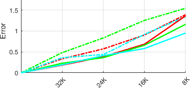
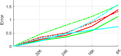
Second, we selected 3 patches from the Artifacts dataset and sub-sampled them with , , and vertices (see Figure 9).These four meshes are compared against the original patch (that has vertices).These four distance values provide an estimate of the error the descriptors do when working with the simplified meshes.
We performed two runs for both the edgeLBP and meshLBP:
- •
Run1: , . These settings are the setting used by the meshLBP as default. Both meshLBP and edgeLBP are run with these settings. For the edgeLBP we set .
- •
Run2: , . These settings are those that we consider default for the edgeLBP. Both the algorithms are run with these settings. As in , we set .
Figure 10 represents the distance between the original model and its four approximations with respect to both edgeLBP and meshLBP, for all the three original meshes. Since the scale of the distances adopted by the meshLBP and edgeLBP is different, we normalize them with respect the range of the distance values among these patches.
| Run1 |
 |
| Run2 |
 |
 |
From Figure 10, we can see that in both runs the edgeLBP produces more stable descriptors, as the errors are lower than those of the meshLBP (except in one case, the model 1 in Run2). In our opinion the nature of the ring definition of the two methods is crucial being both methods based on the LBP concept. Indeed, the meshLBP creates rings of different size when the vertex density decreases becoming quite sparse when the number of vertices of the mesh is significantly reduced. This is not the case of the edgeLBP, as the radius of each ring is always the same (), for each mesh.
5 Discussions and conclusive remarks
We defined an extension of the LBP on surfaces, whose strength is the robustness to the surface tessellation. In this paper we used this technique to successfully retrieve and classify colorimetric patterns on mesh surfaces. The edgeLBP also performed the best to the SHREC’18 track on retrieval of colorimetric patterns [20]. Besides synthetic datasets, we tested our algorithm on samples coming from a challenging dataset made of corrupted and degraded artifacts of the EU GRAVITATE project test beds [1], achievingpromising results. Further extensions are planned and possible. For instance, it is possible to adopt this approach for the description of geometric patterns, encoding the geometric variations with scalar properties of the mesh, like mean curvature or shape index. Moreover, we think that for full color patterns better results could be achieved using all the colorimetric information, for instance the L, a, and b channels of the CIELab space. In this direction, we are currently working on the extension of the edgeLBP to multidimensional properties.
Finally, we think it is worth investigating the automatic recognition and localization of multiple patterns on surfaces. Current experiments are performed on surfaces fully characterized by a single pattern at a time and the similarity distance is defined on the global fragment skin. Next plans include the combination of the shape description step with segmentation techniques and the aggregation of parts made of vertices with similar local descriptions.
Acknowledgments
The work is developed within the research program of the “H2020” European project “GRAVITATE”, contract n. 665155, (2015-2018).
References
- [1] GRAVITATE: Discovering relationships between artefacts using 3D and semantic data. EU H2020 REFLECTIVE project.
- [2] meshLBP. https://it.mathworks.com/matlabcentral/fileexchange/48875-mesh-lbp.
- [3] E. Albuz, E. D. Kocalar, and A. A. Khokhar. Quantized cielab* space and encoded spatial structure for scalable indexing of large color image archives. In ICASSP ’00, volume 6, pages 1995–1998, 2000.
- [4] R. A. Baeza-Yates and B. Ribeiro-Neto. Modern Information Retrieval. Addison-Wesley Longman Publishing Co., Inc., Boston, MA, USA, 1999.
- [5] S. Biasotti, A. Cerri, D. Giorgi, and M. Spagnuolo. Phog: Photometric and geometric functions for textured shape retrieval. Computer Graphics Forum, 32(5):1383–1392, 2013.
- [6] S. Biasotti and et al. Retrieval and Classification on Textured 3D Models. In B. Bustos, H. Tabia, J.-P. Vandeborre, and R. Veltkamp, editors, 3DOR’14. The Eurographics Association, 2014.
- [7] S. Biasotti and et al. Retrieval and classification methods for textured 3D models: a comparative study. The Visual Computer, 32(2):217–241, 2016.
- [8] D. Bommes, B. Lévy, N. Pietroni, E. Puppo, C. Silva, M. Tarini, and D. Zorin. Quad-Mesh generation and processing: A survey. Computer Graphics Forum, 32(6):51–76, 2013.
- [9] A. Cerri and et al. SHREC’13 Track: Retrieval on Textured 3D Models. In 3DOR’13, EG 3DOR’13, pages 73–80, Girona, Spain, 2013. Eurographics Association.
- [10] P. Cignoni, M. Callieri, M. Corsini, M. Dellepiane, F. Ganovelli, and G. Ranzuglia. MeshLab: an Open-Source Mesh Processing Tool. In V. Scarano, R. D. Chiara, and U. Erra, editors, EGIT’08. The Eurographics Association, 2008.
- [11] N. Dalal and B. Triggs. Histograms of oriented gradients for human detection. In CVPR, volume 1, pages 886–893, 2005.
- [12] V. Garro and A. Giachetti. Scale space graph representation and kernel matching for non rigid and textured 3D shape retrieval. IEEE Trans. Pattern Anal. Mach. Intell., 38(6):1258–1271, 2016.
- [13] A. Giachetti and et al. Retrieval of Non-rigid (textured) Shapes Using Low Quality 3D Models. In I. Pratikakis, M. Spagnuolo, T. Theoharis, L. V. Gool, and R. Veltkamp, editors, 3DOR’15. The Eurographics Association, 2015.
- [14] D. Giorgi, S. Biasotti, and L. Paraboschi. Watertight models track. Research Report 09, IMATI, Genova, 2007.
- [15] R. W. G. Hunt and M. R. Pointer. Measuring Colour, Fourth Edition. Wiley, 2011.
- [16] K. Järvelin and J. Kekäläinen. Cumulated gain-based evaluation of IR techniques. ACM Trans. Inf. Syst., 20:422–446, 2002.
- [17] L. Liu, P. Fieguth, Y. Guo, X. Wang, and M. Pietikäinen. Local binary features for texture classification: Taxonomy and experimental study. Pattern Recognition, 62:135 – 160, 2017.
- [18] D. G. Lowe. Distinctive image features from scale-invariant keypoints. Int. J. Comput. Vision, 60(2):91–110, 2004.
- [19] M. Mortara, G. Patané, M. Spagnuolo, B. Falcidieno, and J. Rossignac. Blowing bubbles for multi-scale analysis and decomposition oftriangle meshes. Algorithmica, 38(1):227–248, 2004.
- [20] E. Moscoso Thompson, C. Tortorici, N. Werghi, S. Berretti, S. V. Forero, and S. Biasotti. SHREC’18 track: Retrieval of gray patterns depicted on 3D models. In A. Telea and T. Theoharis, editors, 3DOR’18. The Eurographics Association, 2018.
- [21] T. Ojala, M. Pietikäinen, and D. Harwood. A comparative study of texture measures with classification based on featured distributions. Pattern Recognition, 29(1):51–59, 1996.
- [22] T. Ojala, M. Pietikainen, and T. Maenpaa. Multiresolution gray-scale and rotation invariant texture classification with local binary patterns. IEEE T. Pattern Anal. Mach. Intell., 24(7):971–987, 2002.
- [23] P. Papadakis, I. Pratikakis, T. Theoharis, and S. Perantonis. Panorama: A 3D shape descriptor based on panoramic views for unsupervised 3D object retrieval. Int. J. Comput. Vis., 89(2):177–192, 2010.
- [24] G. Pasqualotto, P. Zanuttigh, and G. M. Cortelazzo. Combining color and shape descriptors for 3D model retrieval. Signal Process-Image, 28(6):608 – 623, 2013.
- [25] S. C. Phillips and et al. GRAVITATE: Geometric and Semantic Matching for Cultural Heritage Artefacts. In C. E. Catalano and L. D. Luca, editors, GCH’16. The Eurographics Association, 2016.
- [26] C. J. V. Rijsbergen. Information Retrieval. Butterworth-Heinemann, Newton, MA, USA, 2nd edition, 1979.
- [27] Y. Rubner, C. Tomasi, and L. J. Guibas. The Earth Mover’s distance as a metric for image retrieval. Int. J. Comput. Vis., 40(2):99–121, Nov. 2000.
- [28] G. Salton. The evaluation of automatic retrieval procedures— selected test results using the smart system. American Documentation, 16(3):209–222, 1965.
- [29] J. Starck and A. Hilton. Correspondence labelling for wide-timeframe free-form surface matching. In ICCV, pages 1–8, 2007.
- [30] M. Suzuki. A Web-based retrieval system for 3D polygonal models. In NAFIPS, volume 4, pages 2271–2276, 2001.
- [31] F. Tombari, S. Salti, and L. Di Stefano. A combined texture-shape descriptor for enhanced 3D feature matching. In ICIP, pages 809–812, 2011.
- [32] Y. Wang, S. Asafi, O. van Kaick, H. Zhang, D. Cohen-Or, and B. Chen. Active co-analysis of a set of shapes. ACM Trans. Graph., 31(6):165:1–165:10, 2012.
- [33] N. Werghi, S. Berretti, and A. D. Bimbo. The mesh-LBP: A framework for extracting local binary patterns from discrete manifolds. IEEE Trans. Image Processing, 24(1):220–235, 2015.
- [34] N. Werghi, C. Tortorici, S. Berretti, and A. D. Bimbo. Local binary patterns on triangular meshes: Concept and applications. Comput Vis Image Underst, 139:161–177, 2015.
- [35] N. Werghi, C. Tortorici, S. Berretti, and A. D. Bimbo. Boosting 3D LBP-based face recognition by fusing shape and texture descriptors on the mesh. IEEE Trans. Inf. Forensics Security, 11(5):964–979, 2016.
- [36] C. Wu, B. Clipp, X. Li, J.-M. Frahm, and M. Pollefeys. 3D model matching with Viewpoint-Invariant Patches (VIP). In CVPR, pages 1–8, 2008.
- [37] A. Zaharescu, E. Boyer, and R. Horaud. Keypoints and local descriptors of scalar functions on 2D manifolds. Int. J. Comput. Vision, 100(1):78–98, 2012.