Constraint Splitting and Projection Methods for Optimal Control of Double Integrator
Abstract
We consider the minimum-energy control of a car, which is modelled as a point mass sliding on the ground in a fixed direction, and so it can be mathematically described as the double integrator. The control variable, representing the acceleration or the deceleration, is constrained by simple bounds from above and below. Despite the simplicity of the problem, it is not possible to find an analytical solution to it because of the constrained control variable. To find a numerical solution to this problem we apply three different projection-type methods: (i) Dykstra’s algorithm, (ii) the Douglas–Rachford (DR) method and (iii) the Aragón Artacho–Campoy (AAC) algorithm. To the knowledge of the authors, these kinds of (projection) methods have not previously been applied to continuous-time optimal control problems, which are infinite-dimensional optimization problems. The problem we study in this article is posed in infinite-dimensional Hilbert spaces. Behaviour of the DR and AAC algorithms are explored via numerical experiments with respect to their parameters. An error analysis is also carried out numerically for a particular instance of the problem for each of the algorithms.
Dedicated to the memory of Jonathan M. Borwein
Key words: Optimal control, Dykstra projection method, Douglas-Rachford method, Aragón Artacho–Campoy algorithm, Linear quadratic optimal control, control constraints, Numerical methods.
1 Introduction
In this paper, we provide (to the best of our knowledge also first) application of various best approximation algorithms to solve a continuous-time optimal control problem. Operator splitting methods were applied previously to discrete-time optimal control problems [17, 24], which are finite-dimensional problems. In [24], for example, the state difference equations comprise the constraint , and the box constraints on the state and control variables comprise . The condition of belonging to the sets and are then appended to the objective function via indicator functions. The original objective function that is considered in [24] is quadratic in the state and control variables. In the next step in [24], the new objective function is split into its quadratic and convex parts and the Douglas-Rachford splitting method is applied to solve the problem.
In the current paper, we deal with continuous-time optimal control problems, which are infinite-dimensional optimization problems that are set in Hilbert spaces. After splitting the constraints of the problem, we apply Dykstra’s algorithm [9], the Douglas–Rachford (DR) method [15, 23, 16, 4, 27, 7], and the Aragón Artacho–Campoy (AAC) algorithm [2], all of which solve the underlying best approximation problem.
The exposure of the current paper is more in the style of a tutorial. We pose the problem of minimum-energy control of a simplified model of a car, amounting to the double integrator, where the control variable has simple lower and upper bounds and the initial and terminal state variables are specified. We split the constraints into two, and , representing respectively the state differential equations (the double integrator) along with their boundary conditions and the constraints on the control variable. We define two subproblems, one subject to , and the other one subject to . We take advantage of the relatively simple form of the optimal control problem and derive analytical expressions for the optimality conditions and implement these in defining the projections onto and .
The solutions of these subproblems provide the projections of a given point in the control variable space onto the constraint sets and , respectively, in some optimal way. By performing these projections in the way prescribed by the above-listed algorithms, we can ensure convergence to a solution of the original optimal control problem,
Note that while the minimum-energy control of the double integrator without any constraints on the control variable can be solved analytically, the same problem with (even simple bound, i.e., box) constraints on the control variable can in general be solved only numerically. This problem should be considered within the framework of control-constrained linear-quadratic optimal control problems for which new numerical methods are constantly being developed—see for example [10, 1] and the references therein.
The current paper is a prototype for future applications of projection methods to solving more general optimal control problems. Indeed, the minimum-energy control of double integrator is a special case of linear quadratic optimal control problems; so, with the reporting of the current study, an extension to more general problems will be imminent.
The paper is organized as follows. In Section 2, we state the control-constrained minimum-energy problem for the double integrator, and write down the optimality conditions. We provide the analytical solution for the unconstrained problem. For the control-constrained case, we briefly describe the standard numerical approach and consider an instance of the problem which we use in the numerical experiments in the rest of the paper. We define the constraint sets and . In Section 3, we provide the expressions for the projections onto and . We describe the algorithms in Section 4 and in the beginning of Section 5. In the remaining part of Section 5, we present numerical experiments to study parametric behaviour of the algorithms as well as the errors in the state and control variables with each algorithm. In Section 6, we provide concluding remarks and list some open problems.
2 Minimum-Energy Control of Double Integrator
We consider the minimum-energy control of a car, with a constrained control variable. Consider the car as a point unit mass, moving on a frictionless ground in a fixed line of action. Let the position of the car at time be given by and the velocity by . By Newton’s second law of motion, , where is the summation of all the external forces applied on the car, in this case the force simply representing the acceleration and deceleration of the car. This differential equation model is referred to as the double integrator in system theory literature, since can be obtained by integrating twice.
Optimal Control Problem. Suppose that the total force on the car, i.e., the acceleration or deceleration of the car, is constrained by a magnitude of . Let and . Then the problem of minimizing the energy of the car, which starts at a position with a velocity and finishes at some other position with velocity , within one unit of time, can be posed as follows.
Here, the functions and are referred to as the state variables and the control variable. As a first step in writing the conditions of optimality for this optimization problem, define the Hamiltonian function for Problem (P) simply as
| (1) |
where is the adjoint variable (or costate) vector such that (see [19])
| (2) |
Equations in (2) simply reduce to
| (3) |
where and are real constants. Let the state variable vector .
Maximum Principle. If is an optimal control for Problem (P), then there exists a continuously differentiable vector of adjoint variables , as defined in (2), such that for all , and that, for a.e. ,
| (4) |
i.e.,
| (5) |
see e.g. [19]. Condition (5) implies that the optimal control is given by
| (6) |
From (6), we can also conclude that the optimal control for Problem (P) is continuous.
When is large enough, the control constraint does not become active, so the optimal control is simply , and it is a straightforward classroom exercise to find the analytical solution as
for all , where
The solution of an instance of Problem (P), with , , , , and large , say , is depicted in Figure 1. Note that, for all , and . The graphs of and are not displayed for this particular instance.

(a) Optimal state variables.

(b) Optimal control variable.
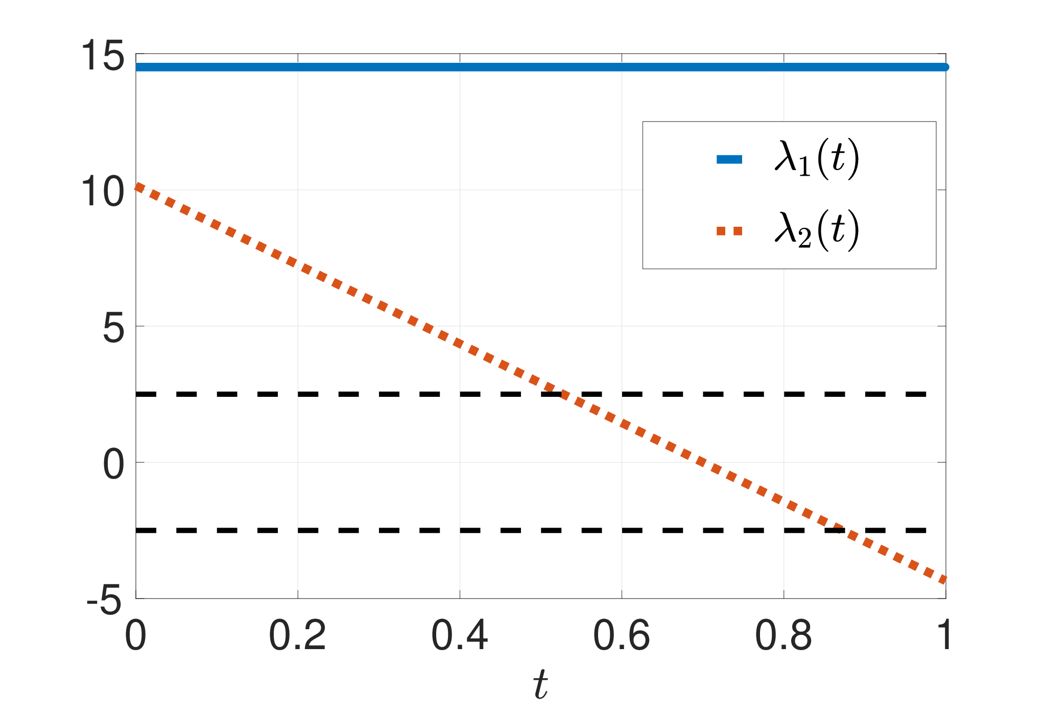
When is not so large, say , as we will consider next so that the control constraint becomes active, it is usually not possible to find an analytical solution, i.e., a solution has to be found numerically, as described below.

(a) Optimal state variables.

(b) Optimal control variable.
(c) Adjoint variables.
Numerical Approach. A straightforward and popular numerical approach to solving Problem (P) is to discretize Problem (P) over a partition of the time horizon and then use some finite-dimensional optimization software to get a discrete (finite-dimensional) solution for the state and control variables and . The discrete solution is an approximation of the continuous-time solution. This approach is often referred to as the direct method or the (first-)discretize-then-optimize approach. A survey and discussion of Euler discretization of linear-quadratic optimal control problems and convergence of their discretized solutions to their continuous-time solutions can be found in [10, Section 5].
Figure 2 depicts the discrete solution of Problem (P) with the instance where , , , , . The solution was obtained by pairing up the optimization modelling language AMPL [18] and the finite-dimensional optimization software Ipopt[28]. The number of discretization nodes was taken to be 2000. The multipliers of the (Euler approximation of the) state differential equation constraints are provided by Ipopt when it finds an optimal solution to the discretized (finite-dimensional) problem. These multipliers have been plotted in Figure 2(c). It should be noted that the graph of the adjoint variable given in Figure 2(c) verifies the graph of the optimal control in Figure 2(b) via the optimal control rule in (6). In Figures 2(b) and (c), the bounds have been marked by horizontal dashed lines for ease of viewing.
Function Spaces. For the numerical methods, we consider projection/reflection methods in Hilbert spaces. The spaces associated with Problem (P) are set up as follows. Let and be the Banach space of Lebesgue measurable functions
with finite norm. Namely, define
where
for , with the modulus or absolute value. In other words,
Furthermore, is the Sobolev space of absolutely continuous functions, namely
endowed with the norm
In Problem (P), the state variable and the control variable .
Constraint Splitting. Next, we split the constraints of Problem (P) into two subsets, and . The subset collects together all the feasible control functions satisfying only the dynamics of the car. The subset , on the other hand, collects all the control functions whose values are constrained by and .
| (7) | |||||
| (8) |
The rationale behind this sort of splitting is as follows: The problem of minimizing the energy of the car subject to only or only is much easier to solve – in fact, the solutions can be analytically written in each case. If, for some given , a solution exists to the two-point boundary-value (TPBVP) in (7) then that solution is unique by the linearity of the TPBVP [3, 26]. Note that a control solution as in (7) exists by the (Kalman) controllability of the double integrator – see [25]. So the set is nonempty. Note that the constraint set is an affine subspace and a box.
3 Projections
All of the projection methods that we will consider involve projections onto the sets and . The projection onto from a current iterate is the point solving the following problem.
In (P1), we minimize the squared -norm distance between and . The projection onto from a current iterate is similarly the point solving the following problem.
Proposition 1 (Projection onto )
The projection of onto the constraint set , as the solution of Problem (P1), is given by
| (9) |
for all , where
| (10) | |||
| (11) |
and and are obtained by solving the initial value problem
| (12) | |||
| (13) |
for all .
Proof. The Hamiltonian function for Problem (P1) is
where the adjoint variables and are defined as in (2), with replaced by , and the subsequent solutions are given as in (3). The optimality condition for Problem (P1) is akin to that in (4) for Problem (P) and, owing to the fact that the control is now unconstrained, can more simply be written as
which yields the optimal control as , i.e.
| (14) |
for all . We need to show that and are found as in (10)–(11). Using (14) in (7) yields the following time-varying, linear two-point boundary-value problem.
| (15) | |||
| (16) |
for all . In other words, Problem (P1) is reduced to solving Equations (15)–(16) for the unknown parameters and . Once and are found, the projected point in (14) is found. Since Equations (15)–(16) are linear in and , a simple shooting technique [3, 26] provides the solution for and in just one iteration. The essence of this technique is that the initial-value problem (IVP)
| (17) | |||
| (18) |
for all , is solved repeatedly, so as to make the discrepancy at vanish. Namely, we seek a parameter such that and . The procedure is as follows. For a given , there exists a unique solution of (17)–(18). Define the near-miss (vector) function as follows:
| (19) |
The Jacobian of the near-miss function is
The shooting method looks for a pair such that (i.e., a pair such that the final boundary conditions are met). Expanding about, say, , and discarding the terms of order or higher, we obtain
Substituting in the above expression, replacing “” with “”, and re-arranging, gives the single (Newton) iteration of the shooting method:
| (20) |
The components , , of , can be obtained by solving the variational equations for (15)–(16) with respect to and , i.e., by solving the following system for :
Elementary calculations lead to the following solution of the above system:
which is independent of . Hence,
with inverse:
| (21) |
Setting , the IVP (17)–(18) becomes (12)–(13). Then substitution of (19) and (21) with into Equation (20), and expanding out, yield (10)–(11). The proof is complete.
Proposition 2 (Projection onto )
The projection of onto the constraint set , as the solution of Problem (P2), is given by
| (22) |
for all .
Proof. The expression (22) is the straightforward solution of Problem (P2).
4 Best Approximation Algorithms
In this section, we discuss best approximation algorithms. In the following,
| is a real Hilbert space | (23) |
with inner product , induced norm . We also assume that
| is a closed affine subspace of , and is a nonempty closed convex subset of . | (24) |
Given , our aim is to find
| (25) |
the projection of onto the intersection which we assume to be nonempty. We also assume that we are able to compute the projectors onto the constraints and .
Many algorithms are known which could be employed to find ; here, however, we focus on three simple methods that do not require a product space set-up as some of those considered, in, e.g., [4, 5, 11, 12].
In the next section, we will numerically test these algorithms when , , , and .
4.1 Dykstra’s Algorithm
We start with Dykstra’s algorithm (see [9]), which operates as follows11 1 In the general case, there is also an auxiliary sequence associated with ; however, because is an affine subspace, it is not needed in our setting.: Set and . Given , where , update
| (26) |
It is known that both and converge strongly to .
4.2 Douglas–Rachford Algorithm
Given , we specialize the Douglas–Rachford algorithm (see [15], [23] and [16]) to minimize the sum of the two functions and which have respective proximal mappings (see [4, Proposition 24.8(i)]) and . Set . It follows that the Douglas–Rachford operator turns into
| (27) |
Now let and given , where , update
| (28) |
Then it is known (see [27] or [7]) that converges weakly to . Note that (28) simplifies to
| (29) |
4.3 Aragón Artacho–Campoy Algorithm
The Aragón Artacho–Campoy (AAC) Algorithm was recently presented in [2]. Given two fixed parameters and in , define
| (30) |
Now let and given , where , update
| (31) |
and
| (32) |
By [2, Theorem 4.1(iii)], the sequence converges strongly to provided that22 2 It appears that this constraint qualification is not easy to check in our setting. . Note that (32) simplifies to
| (33) |
5 Numerical Implementation
5.1 The algorithms
In this section, we gather the algorithms considered abstractly and explain how we implemented them.
We start with Dykstra’s algorithm from Subsection 4.1.
Algorithm 1 (Dykstra)
- Step 1
-
(Initialization) Choose the initial iterates and . Choose a small parameter , and set .
- Step 2
-
(Projection onto ) Set . Compute by using (22).
- Step 3
-
(Projection onto ) Set . Compute by using (9).
- Step 4
-
(Update) Set and .
- Step 5
-
(Stopping criterion) If , then return and stop. Otherwise, set and go to Step 2.
Next is the Douglas–Rachford method from Subsection 4.2.
Algorithm 2 (DR)
- Step 1
-
(Initialization) Choose a parameter and the initial iterate arbitrarily. Choose a small parameter , and set .
- Step 2
-
(Projection onto ) Set . Compute by using (22).
- Step 3
-
(Projection onto ) Set . Compute by using (9).
- Step 4
-
(Update) Set .
- Step 5
-
(Stopping criterion) If , then return and stop. Otherwise, set and go to Step 2.
Finally, we describe the Aragón Artacho–Campoy algorithm from Subsection 4.3.
Algorithm 3 (AAC)
- Step 1
-
(Initialization) Choose the initial iterate arbitrarily. Choose a small parameter , two parameters33 3 Aragón Artacho and Campoy recommend and ; see [2, End of Section 7]. and in , and set .
- Step 2
-
(Projection onto ) Set . Compute by using (22).
- Step 3
-
(Projection onto ) Set . Compute by using (9).
- Step 4
-
(Update) Set .
- Step 5
-
(Stopping criterion) If , then return and stop. Otherwise, set and go to Step 2.
We provide another version of each of Algorithms 1–3, as Algorithms 1b–3b, in Appendix A. In Algorithm 1b, we monitor the sequence of iterates which are the projections onto set , instead of monitoring the projections onto set in Algorithm 1. On the other hand, in Algorithms 2b–3b, the order in which the projections are done is reversed: the first projection is done onto the set and the second projection onto .
Although the order of projections will not matter in view of the existing results stating that convergence is achieved under any order – see [6, Proposition 2.5(i)], the order does make a difference in early iterations (as well as in the number of iterations required for convergence of Algorithms 2 and 2b, as we will elaborate on later). If our intent is to stop the algorithm early so that we can use the current iterate as an initial guess in more accurate computational optimal control algorithms, which can find the junction times with a high precision (see [21, 22, 20]), then it is desirable to implement Algorithms 1–3 above, rather than Algorithms 1b–3b, because any iterate of Algorithms 1–3 will satisfy the constraints on the control variable, while that of Algorithms 1b–3b will in general not.
5.2 Numerical experiments
In what follows, we study the working of Algorithms 1–3 for an instance of Problem (P). Suppose that the car is initially at a reference position 0 and has unit speed. It is desired that the car come back to the reference position and be at rest after one unit of time; namely that , , , . For these boundary conditions, no solution exists if one takes the control variable bound or smaller but a solution does exist for . So, we use . In the ensuing discussions, we use the stopping tolerance unless otherwise stated.
Discretization. Algorithms 1–3, as well as 1b–3b, carry out iterations with functions. For computations, we consider discrete approximations of the functions over the partition such that
and is the number of subdivisions. Let be an approximation of , i.e., , ; similarly, and , or , . In other words, the functions , and are approximated by the -dimensional array , with components , , and the -dimensional arrays and , with components and , , respectively. We define a discretization of the projection as follows.
| (34) |
where ,
| (35) | |||
| (36) |
and and are obtained from the Euler discretization of (12)–(13): Given and ,
| (37) | |||
| (38) |
for .
The discretization of the projection can be defined in a straightforward manner, by simply replacing in (22) with the discrete components of .
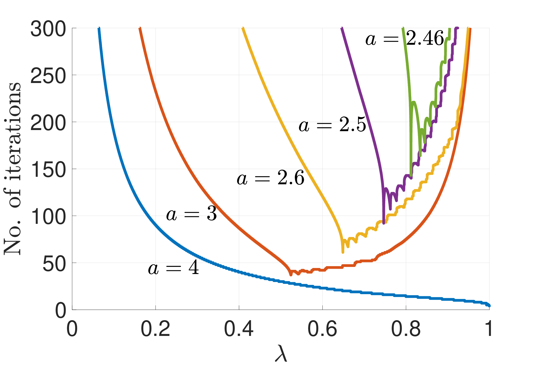
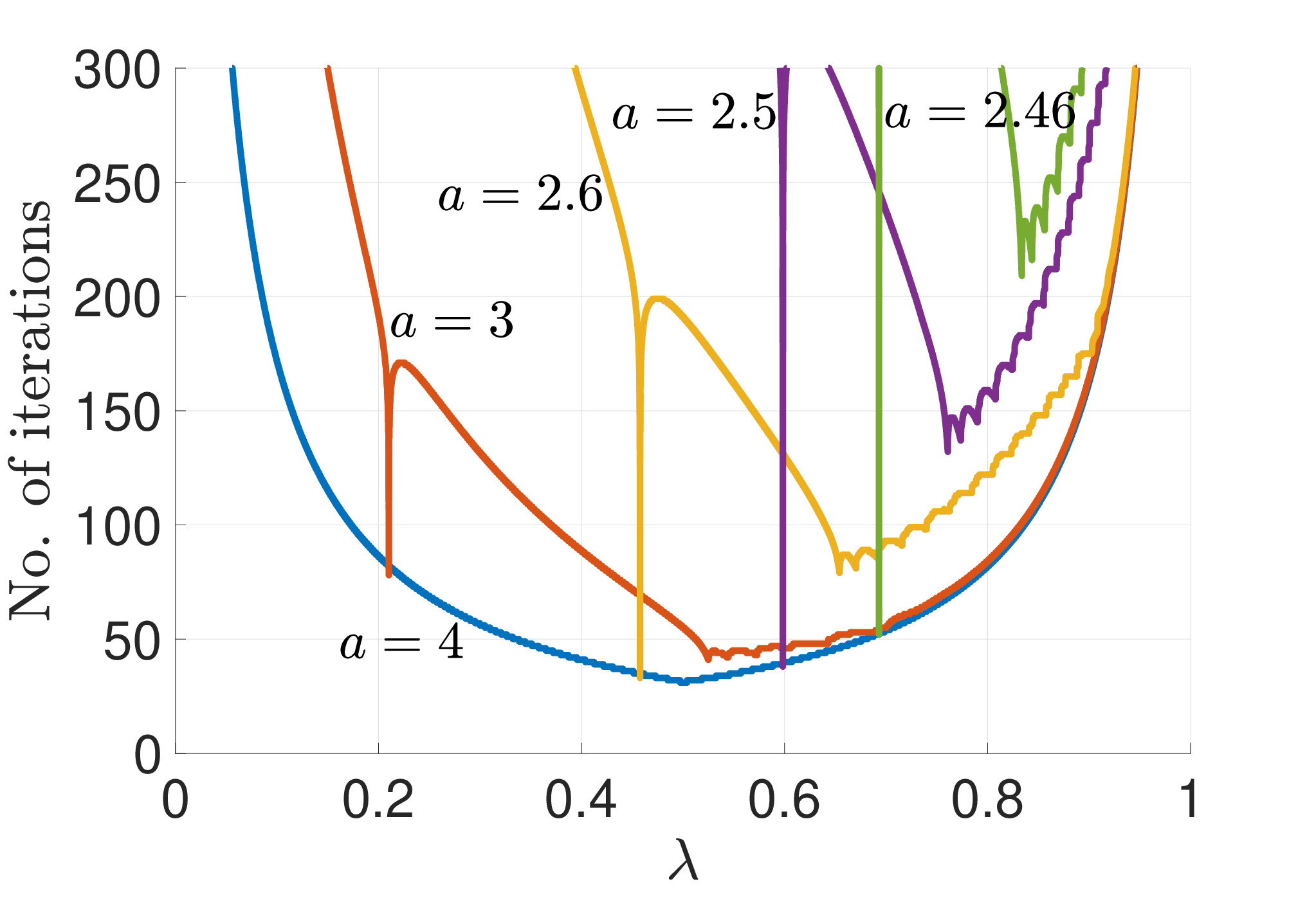
Parametric Behaviour. Obviously, the behaviour of Algorithms 2 and 2b, the Douglas–Rachford method, depend on the parameter , and the behaviour of Algorithms 3 and 3b on the two parameters and . Figure 3 displays the dependence of the number of iterations it takes to converge on these parameters, for various values of . The dependence for a given value of appears to be continuous, albeit the presence of downward spikes.
The graphs for Algorithms 2 and 2b, shown in parts (a) and (c) of Figure 3, respectively, differ significantly from one another. The bound corresponds to the case when the control constraint becomes active only at – see Figure 1. In other words, when the optimal control variable is truly unconstrained. When , the best value of is 1 for Algorithm 2, yielding the solution in just 6 iterations. For Algorithm 2b, the best value for is 0.5, as can be seen in (c), producing the solution in 30 iterations. Going back to Algorithm 2, with decreasing values of , the values of minimizing the number of iterations shift to the right. For example, the minimum number of iterations is 91, with and (found by a refinement of the graph).
As for Algorithm 2b, the minimizer for is and the corresponding minimum number of iterations is 38. This is a point where a downward spike occurs and so the number of iterations is very sensitive to changes in . For example, the rounded-off value of results in 88 iterations instead of 38, and yields 444 iterations for convergence. The number of iterations is less sensitive to the local minimizer , which results in 132 iterations. It is interesting to note that the graph with appears to be an envelope for the number of iterations for all .
(a) Algorithm 2 (DR)

(b) Algorithms 3 (AAC) and 3b (AAC-b)
for
(c) Algorithm 2b (DR-b)

(d) Algorithms 3 (AAC) and 3b (AAC-b)
The graphs for Algorithms 3 and 3b, the Aragón Artacho–Campoy algorithm, are indistinguishable to one’s eye; therefore we only display the one in Figure 3(b). Part (d) of Figure 3 shows surface plots of the number of iterations versus the algorithmic parameters and , for the same values of as in the rest of the graphs in the figure. It is interesting to observe that the surfaces look to be cascaded with (roughly) the outermost surface being the one corresponding to . The surface plot suggests that for minimum number of iterations, one must have . Although theory requires , seems to cause no concerns in this particular intance; so, we set for the rest of the paper. The cross-sectional curves at are shown with much more precision in part (b) of the figure. The spikes that are observed in part (d) can also be seen in the graph in part (b).
In fact, the first observation one has to make here is that, for , convergence can be achieved in merely one iteration, with . This is quite remarkable, compared with Algorithms 2 and 2b. The graphs in (b) appear to be enveloped as well by the graph for , as in part (c). For the values of other than 4, the globally minimum number of iterations seems to be achieved at a downward spike, which as a result is very sensitive to changes in . For example, for , the optimal value is 0.78249754 for a minimum 35 iterations. A rounded-off results in 111 iterations, and yields 243 iterations. Sensitivity at the local minimizer giving 64 iterations is far less: Choosing or results in 128 or 90 iterations, respectively. It is interesting to note that, as in the case of Algorithms 2 and 2b, the graphs in Figure 3(b) are approximately enveloped by the graph/curve drawn for .

(a) Algorithm 1 (Dykstra)
stops after 530 iterations.

(b) Algorithm 2 (DR, )
stops after 91 iterations.

(c) Algorithm 3 (AAC, , )
stops after 64 iterations.

(d) -error in control by Algorithms 1–3.

(e) -error in states by Algorithms 1–3.
Behaviour in Early Iterations. Figure 4(a)–(c) illustrates the working of all three algorithms for the same instance. All three algorithms converge to the optimal solution, with the stopping tolerance of . The optimal values of the algorithmic parameters, for Algorithm 2, and and for Algorithm 3, have been used. The third, fifth and fifteenth iterates, as well as the solution curve, are displayed for comparisons of behaviour. At least for the given instance of the problem, it is fair to say from Figure 4(c) that Algorithm 3 gets closer to the solution much more quickly than the others in the few initial iterations—see the third and fifth iterates. It also achieves convergence in a smaller number of iterations (64 as opposed to 530 and 91 iterations of the Algorithms 1 and 2, respectively).
Error Analysis via Numerical Experiments. For a fixed value of , Algorithms 1–3 converge only to some approximate solution of the original Problem. Therefore, the question as to how the algorithms behave as the time partition is refined, i.e., is increased, needs to be investigated. For the purpose of a numerical investigation, we define, in the th iteration, the following errors. Suppose that the pair is the optimal solution of Problem (P) and an approximate solution of Problem (P) in the th iteration of a given algorithm. Define
where is the -norm in . For large , these expressions are reminiscent of the -norm, and therefore they will be referred to as the -error.
For in the error expressions, we have used the discretized (approximate) solution obtained for the Euler-discretized Problem (P) utilizing the Ipopt–AMPL suite, with and the tolerance set at .
For , these errors are depicted in Figure 4(d) and (e). From the graphs it is immediately clear that no matter how much smaller the stopping tolerance is selected, the best error that is achievable with is around for the control variable and around for the state variable vector. In fact, the graphs also tell that perhaps a much smaller stopping threshold than would have achieved the same approximation to the continuous-time solution of Problem (P). By just looking at the graphs, one can see that Algorithm 1 could have been run just for about 300 iterations instead of 530, and Algorithms 2 and 3 could have been run for about 50 iterations to achieve the best possible approximation with .
In Figure 5, we depict the same errors for (parts (a) and (b)), (in parts (c) and (d)) and (in parts (e) and (f)). It is observed that, with a ten-fold increase in (which is a ten-fold decrease in ) the errors in both and are reduced by ten-folds, implying that the error (both in and in ) depends on the stepsize linearly. This is in line with the theory of Euler-discretization of optimal control problems; see, for example, [13, 14]. Furthermore, even for very large values of , it can be seen from these graphs that a stopping threshold slightly smaller than would suffice to get even more stringent error levels, such as around for the control variable and around for the state variable vector. A larger stopping threshold would obviously result in smaller number of iterations.

(a) -error in control with .

(b) -error in states with .

(c) -error in control with .

(d) -error in states with .

(e) -error in control with .

(f) -error in states with .
Table 1 displays the values of the errors, separately in and , after the stopping criteria with was satisfied, for each of the three algorithms. A precise 10-fold reduction in error with a 10-fold increase in can be verified with these numbers, as discussed in the previous paragraph. We have added the experiments we have carried out with Ipopt, version 3.12, an interior point optimization software [28], which solved the direct Euler-discretization of Problem (P), with the same values of and the same tolerance . Ipopt, running with linear solver MA57, was paired up with the optimization modelling language AMPL [18]. The same 10-fold decreases in error cannot be observed with Ipopt, unless one sets the tolerance for Ipopt to be much smaller than , say (which also means longer computational times). With the tolerance set at , the error values with Ipopt becomes pretty much the same as those with Dykstra (still with ), which is interesting to note.
As we pointed out earlier, the same errors listed in Table 1 can be achieved with bigger stopping thresholds. For , respectively: with , Algorithm 1 converges in 281, 359 and 454 iterations; with , Algorithm 2 converges in 65, 50 and 101 iterations; with , Algorithm 3 converges in 49, 60 and 70 iterations.
In Table 2, the CPU times (in seconds) each algorithm takes, with the respective values listed above, are tabulated. Note that Algorithms 1–3 have been coded and run on Matlab, 64-bit (maci64) version R2017b. All software, including AMPL and Ipopt, were run on MacBook Pro, with operating system macOS Sierra version 10.12.6, processor 3.3 GHz Intel Core i7 and memory 6 GB 2133 MHz LPDDR3. In Table 2, the CPU times for Ipopt are listed with the tolerance , since with only this fine tolerance it is possible to obtain the same order of the error magnitudes as those obtained by Algorithms 1–3. With , the CPU times for Ipopt are 0.06, 0.45 and 4.4 seconds, respectively, which are significantly higher than the times taken by Algorithms 1–3, in addition to worse errors.
Numerical observations suggest two joint winners: Algorithms 2 and 3, i.e., the Douglas–Rachford method and the Aragón Artacho–Campoy algorithm, in both accuracy and speed.
| Dykstra | DR | AAC | Ipopt | |
|---|---|---|---|---|
(a) -error in control, .
Dykstra
DR
AAC
Ipopt
(b) -error in states, .
| Dykstra | DR | AAC | Ipopt | |
|---|---|---|---|---|
| 0.03 | 0.01 | 0.01 | 0.08 | |
| 0.16 | 0.05 | 0.05 | 0.71 | |
| 1.6 | 0.41 | 0.28 | 7.3 |
6 Conclusion and Open Problems
We have applied three well-known projection methods to solve an optimal control problem, i.e., control-constrained minimum-energy control of double integrator. We have derived the projectors for the optimal control problem and demonstrated that they can be used in Dykstra’s algorithm, the Douglas–Rachford (DR) method and the Aragón Artacho–Campoy (AAC) algorithm, effectively. We carried out extensive numerical experiments for an instance of the problem and concluded that the DR and AAC algorithms (Algorithms 2 and 3) were jointly the most successful. We also made comparisons with the standard discretization approach, only to witness the benefit of using projection methods.
It is interesting to note that when we apply alternating projections, we also seem to converge to even though this is not supported by existing theory.
To the best of authors’ knowledge, the current paper constitutes the first of its kind which involves projection methods and continuous-time optimal control problems. It can be considered as a prototype for future studies in this direction. Some of the possible directions are listed as follows.
- •
The setting we have introduced could be extended to general control-constrained linear-quadratic problems.
- •
We have used some discretization of the projector as well as the associated IVP in (34)–(38). This might be extended to problems in more general form. On the other hand, for the particular problem we have dealt with in the present paper, one might take into account the fact that if is piecewise linear then its projection is piecewise linear. This might simplify further the expressions given in Proposition 1.
- •
Although theory for projection methods can in principle vouch convergence only for convex problems, it is well-known that the DR method can be successful for nonconvex problems, see, for example, [8]. It would be interesting to extend the formulations in the current paper to nonconvex optimal control problems.
- •
For a certain value of an algorithmic parameter, Figure 3 exhibits downward spikes. It would be interesting to see if this phenomenon is also observed in other control-constrained optimal control problems.
Appendix
Algorithm 1b (Dykstra-b)
- Steps 1–4
-
(Initialization) Do as in Steps 1–4 of Algorithm 1.
- Step 5
-
(Stopping criterion) If , then return and stop. Otherwise, set and go to Step 2.
Algorithm 2b (DR-b)
- Step 1
-
(Initialization) Choose a parameter and the initial iterate arbitrarily. Choose a small parameter , and set .
- Step 2
-
(Projection onto ) Set . Compute by using (9).
- Step 3
-
(Projection onto ) Set . Compute by using (22).
- Step 4
-
(Update) Set .
- Step 5
-
(Stopping criterion) If , then return and stop. Otherwise, set and go to Step 2.
Algorithm 3b (AAC-b)
- Step 1
-
(Initialization) Choose the initial iterate arbitrarily. Choose a small parameter , two parameters and in , and set .
- Step 2
-
(Projection onto ) Set . Compute by using (9).
- Step 3
-
(Projection onto ) Set . Compute by using (22).
- Step 4
-
(Update) Set .
- Step 5
-
(Stopping criterion) If , then return and stop. Otherwise, set and go to Step 2.
References
- [1] W. Alt, C. Y. Kaya and C. Schneider, Dualization and discretization of linear-quadratic control problems with bang–bang solutions. EURO J Comput. Optim., 4 (2016), 47–77.
- [2] F. J. Aragón Artacho and R. Campoy, A new projection method for finding the closest point in the intersection of convex sets. Comput. Optim. Appl. 69 (2018), 99–132.
- [3] U. M. Ascher, R. M. M. Mattheij and R. D. Russell, Numerical Solution of Boundary Value Problems for Ordinary Differential Equations. SIAM Publications, Philadelphia, 1995.
- [4] H. H. Bauschke and P. L. Combettes, Convex Analysis and Monotone Operator Theory in Hilbert Spaces. Second edition. Springer, 2017.
- [5] H. H. Bauschke and V. R. Koch, Projection methods: Swiss Army knives for solving feasibility and best approximation problems with halfspaces. Infinite Products of Operators and Their Applications, 2012, 1–40.
- [6] H. H. Bauschke and W. M. Moursi, On the order of the operators in the Douglas–Rachford algorithm. Optimization Letters, 10 (2016), 447–455.
- [7] H. H. Bauschke and W. M. Moursi, On the Douglas–Rachford algorithm. Math. Program., Ser. A, 164 (2017), 263–284.
- [8] J. M. Borwein and B. Sims, The DouglasÐRachford Algorithm in the absence of convexity. In: Bauschke H., Burachik R., Combettes P., Elser V., Luke D., Wolkowicz H. (eds) Fixed-Point Algorithms for Inverse Problems in Science and Engineering. Springer Optimization and Its Applications, vol 49. Springer, New York, NY.
- [9] J. P. Boyle and R. L. Dykstra, A method for finding projections onto the intersection of convex sets in Hilbert spaces, in Advances in Order Restricted Statistical Inference, vol. 37 of Lecture Notes in Statistics, Springer, 1986, 28–47.
- [10] R. S. Burachik, C. Y. Kaya, and S. N. Majeed, A duality approach for solving control-constrained linear-quadratic optimal control problems. SIAM J. Control Optim., 52 (2014), 1771–1782.
- [11] P. L. Combettes, A block-iterative surrogate constraint splitting method for quadratic signal recovery. IEEE Trans. Sig. Proc., 51 (2003), 2432–2442.
- [12] P. L. Combettes, Iterative construction of the resolvent of a sum of maximal monotone operators. J. Convex Anal., 16 (2009), 727–748.
- [13] A. L. Dontchev and W. W. Hager, The Euler approximation in state constrained optimal control, Math. Comp., 70 (2001), 173–203.
- [14] A. L. Dontchev, W. W. Hager and K. Malanowski, Error bound for Euler approximation of a state and control constrained optimal control problem, Numer. Funct. Anal. Optim., 21 (2000), 653–682.
- [15] J. Douglas and H. H. Rachford, On the numerical solution of heat conduction problems in two and three space variables. Trans. Amer. Math. Soc., 82 (1956), 421–439.
- [16] J. Eckstein and D. P. Bertsekas, On the Douglas-Rachford splitting method and the proximal point algorithm for maximal monotone operators. Math. Program., Ser. A, 55 (1992), 293–318.
- [17] J. Eckstein and M. C. Ferris, Operator-splitting methods for monotone affine variational inequalities, with a parallel application to optimal control. INFORMS J. Comput., 10 (1998), 218–235.
- [18] R. Fourer, D. M. Gay, and B. W. Kernighan, AMPL: A Modeling Language for Mathematical Programming, Second Edition. Brooks/Cole Publishing Company / Cengage Learning, 2003.
- [19] M. R. Hestenes, Calculus of Variations and Optimal Control Theory. John Wiley & Sons, New York, 1966.
- [20] C. Y. Kaya, S. K. Lucas, and S. T. Simakov, Computations for bang–bang constrained optimal control using a mathematical programming formulation, Optim. Contr. Appl. Meth., 25(6) (2004), 295–308.
- [21] C. Y. Kaya and J. L. Noakes, Computations and time-optimal controls, Opt. Cont. Appl. Meth., 17 (1996), 171–185.
- [22] C. Y. Kaya and J. L. Noakes, Computational algorithm for time-optimal switching control, J. Optim. Theory App., 117 (2003), 69–92.
- [23] P.-L. Lions and B. Mercier, Splitting algorithms for the sum of two nonlinear operators. SIAM J. Numer. Anal., 16 (1979), 964–979.
- [24] B. O’Donoghue, G. Stathopoulos, and S. Boyd, A splitting method for optimal control. IEEE Trans. Contr. Sys. Tech., 21 (2013), 2432–2442.
- [25] W. J. Rugh, Linear System Theory, 2nd Edition. Pearson, 1995.
- [26] J. Stoer and R. Bulirsch, Introduction to Numerical Analysis, 2nd Edition. Springer-Verlag, New York, 1993.
- [27] B. F. Svaiter, On weak convergence of the Douglas-Rachford method. SIAM J. Control Optim., 49 (2011), 280–287.
- [28] A. Wächter and L. T. Biegler, On the implementation of a primal-dual interior point filter line search algorithm for large-scale nonlinear programming. Math. Progr., 106 (2006), 25–57.