Seeking Open-Ended Evolution in Swarm Chemistry II:
Analyzing Long-Term Dynamics via Automated Object Harvesting

We used the evolutionary Swarm Chemistry model described in (Sayama,, 2011), which was based on Swarm Chemistry (Sayama,, 2009), a computational model of collective behaviors of self-propelled particles similar to Reynolds’ “Boids” Reynolds, (1987). In Swarm Chemistry, multiple types of particles with different kinetic behavioral parameters are mixed together. Their behavioral parameters are represented in a “recipe,” a set of sequences of kinetic parameter values each of which describes the strength of a specific behavioral rule such as cohesion, alignment, separation (Reynolds,, 1987), etc. Each parameter value sequence in a recipe represents behaviors of one particle type.

In the evolutionary Swarm Chemistry models, these recipes evolve through their transmissions (possibly with stochastic mutations) among colliding particles. The direction of recipe transmission is determined by a competition function that takes local information about two particles engaged in a collision and returns which one becomes the source of the recipe transmission. Examples of competition functions include: “faster” (the faster particle wins = becomes the source of recipe transmission), “slower” (the slower one wins), “majority” (the one that is surrounded by more particles of the same type wins), and so on. The competition function may be varied temporarily as well as spatially to induce exogenous environmental perturbations to promote continuous evolutionary activities.

In this study, we adopted the “revised-high” experimental condition that was identified in (Sayama and Wong,, 2011) to be most successful in producing continuous evolutionary dynamics of macroscopic nontrivial structures. This condition uses a revised collision detection method described in (Sayama and Wong,, 2011), high mutation rates, and spatially heterogeneous environmental perturbations. Each simulation was conducted with 10,000 particles moving and interacting within a 5,000$\times$5,000 (in arbitrary unit) continuous two-dimensional space. Boundary conditions were such that the space was toroidal with regard to particles’ positions (i.e., they would come out from the opposite edge of the space when they went out) but it was also a bounded square with regard to particles’ perception (i.e., they would not sense other particles’ presence across the boundaries), following the model settings used in (Sayama,, 2011). Out of the 10,000 particles, 100 were initialized with randomly generated recipes, while the rest were initially inactive. The primary competition function used to decide the direction of recipe transmission was “majority (relative)” (see (Sayama,, 2011) for details). The simulator code was written in Java and is available from the author’s website¹¹ 1 http://bingweb.binghamton.edu/~sayama/SwarmChemistry/.

In the present study, each simulation was run for 300,000 time steps, ten times longer than the typical simulation length used in earlier work. Snapshots of simulations were saved in the form of a 4,000$\times$4,000-pixel high-resolution bitmap image in every 1,000 time steps, which were analyzed by a separate process described in the next subsection. In those snapshots, particles’ behavioral properties were partly visualized in their colors by mapping the strengths of their cohesion, alignment and separation tendencies to (R, G, B) values.

Like in (Sayama,, 2011; Sayama and Wong,, 2011), exogenous environmental perturbations were periodically introduced in every 2,000 time steps onto either left or right half of the space (randomly selected each time) by changing the competition function within the selected half to either “faster” or “slower” (again, randomly selected each time). In earlier work, each perturbation lasted only for 50 time steps, while in the present study we tested two lengths of environmental perturbations to evaluate the sensitivity of results and the adaptability of evolving structures: (i) 50 time steps (i.e., 1,950 normal steps interjected by 50 steps with perturbation), and (ii) 500 time steps (i.e., 1,500 normal steps interjected by 500 steps with perturbation), which are called “short” and “long” perturbations, respectively, in the following sections.

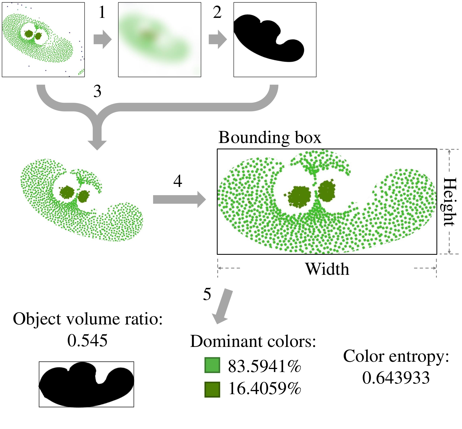
The bitmap images of simulation snapshots generated above were processed concurrently by another process for automated object harvesting. In this work, objects are defined as spatially contiguous morphological structures in which particles were clustered to show some kind of organization. Such objects were detected and extracted in the following image processing steps (also see Fig. 1):

1. 1.

   Blur the snapshot image using blurring radius $r$ to generate a continuous density map.

2. 2.

   Binarize the blurred image to clearly define the areas of interest.

3. 3.

   Dilate each area of interest by radius $r$ to include less dense peripheral parts of the object.

4. 4.

   Using the dilated area of interest as a mask, extract each object from the original snapshot.

We used $r=150$, which was half of the maximum interaction range (300) of the Swarm Chemistry model. Note that this object harvesting method can extract not only small localized objects, but also large-scale global structures as well if they are made of spatially contiguous clusters of particles.

The following measurements were calculated on the simulation snapshots and the harvested objects to characterize the evolutionary dynamics of each simulation run:

• •

  On simulation snapshots (Sayama and Wong,, 2011)

  • –

    Evolutionary exploration (EE):
    Number of new colors that appeared at a specific time point for the first time within the simulation (roughly capturing how many novel particle types appeared)

  • –

    Macroscopic structuredness (MS):
    Kullback-Leibler divergence of an approximated pairwise particle distance distribution from that of a hypothetical case where particles were randomly and homogeneously spread over the space (capturing the extent to which particles formed nontrivial macroscopic structures)

• •

  On harvested objects (these were measured after the object was rotated appropriately to minimize the area of the bounding box; see Fig. 2)

  • –

    Position in space

  • –

    Bounding box width and height (a longer side was always taken for width)

  • –

    Bounding box height-width ratio

  • –

    Bounding box area (= width $\times$ height)

  • –

    Object volume ratio (= area of binarized object image / bounding box area)

  • –

    Number of colors

  • –

    Color entropy

All the image processing tasks involved in the automated object harvesting and object feature analysis were conducted using the image processing functions of Wolfram Research Mathematica 11.3.0.

Figures 3 and 4 show temporal changes of evolutionary exploration (EE) and macroscopic structuredness (MS) measurements, respectively, in simulations under the two perturbation conditions. It was observed in Fig. 3 that EE dropped slightly after the initial 30,000–50,000 time steps, although production of new particle types was sustained at a moderate level for the entire duration of simulation. Fig. 4 shows a significant difference in MS between the short and long perturbation conditions: the former maintained structured particle distributions while the latter failed to do so. This indicates that the too harsh environmental perturbation made it difficult for nontrivial macroscopic structures to be sustained.

Figure 5 shows two representative simulation runs, one from the short perturbation condition and another from the long perturbation condition. As seen in the figure, a typical simulation run more or less settled down into an evolutionarily stable state after about 100,000 time steps, beyond which not much disruptive change occurred even though new particle types were continuously produced by environmental perturbations (Fig. 3). It was often observed that simulation runs under the short perturbation condition eventually ended up with a large-scale homogeneous swarming cloud (Fig. 5 top-right), while the runs under the long perturbation condition did not produce any such large-scale structure at the end (Fig. 5 bottom-right). Note that the earlier work on evolutionary Swarm Chemistry (Sayama,, 2011; Sayama and Wong,, 2011; Sayama,, 2012) only looked at evolutionary dynamics up to 30,000 time steps due to limitations in computational resources, which corresponds to just the first two frames in Fig. 5. Our new long-term simulations suggest that the evolutionary dynamics studied in the earlier work may have been just initial transient behaviors.

Figure 6 shows the temporal changes of the number of harvested objects per snapshot in each simulation run. There was a slight upward trend for most of the runs, and in particular, the long perturbation condition produced a couple of extreme cases in which particles eventually evolved into many scattered tiny clusters. Once the system reached such a scattered, deserted state, it produced no more objects with nontrivial macroscopic structures or behaviors.

Figure 7 shows how some of the features of harvested objects changed over time. In most of the measurements, there were clear long-term trends that were not fully visible within the initial 30,000 time steps that were the focus in the earlier work. For example, in the short perturbation cases (Fig. 7, left), the bounding box width and area went up while the height-width ratio went down, which indicates that the particle population gradually became organized into a large-scale swarm with elongated shapes (see Fig. 5, top). In the meantime, the number of colors and the color entropy did not show any significant changes, implying that the complexity of recipes regarding the number of kinetic types did not show long-term increase. Another important finding is the difference between the short and long perturbation conditions, most notably the much smaller size of objects (as seen in the bounding box width and area in Fig. 7, right) that evolved under the long perturbation conditions. This quantitatively reflects the observation that particles tended to form much tinier clusters under such harsh environmental conditions (see Fig. 5, bottom). It was also observed that the long perturbation conditions resulted in higher numbers of colors and higher color entropy than the short one (Fig. 7, bottom two rows).

The results obtained so far may appear to collectively imply that the long-term evolutionary dynamics of the evolutionary Swarm Chemistry model would be rather limited in innovation and creativity. While this may be the case, the automated harvesting method, nonetheless, successfully captured a number of highly creative objects in the simulation runs. Figure 8 showcases some examples that were arbitrarily selected by the author based on subjective aesthetic criteria. Most of the objects shown in this figure were generated in the middle or later stages of long-term simulations, demonstrating the continuous autonomous creativity of evolutionary Swarm Chemistry.

Figure 8 also shows that the objects generated under the short perturbation conditions tended to have well-defined, clearly identifiable structures, whereas those generated under the long perturbation conditions tended to have more scattered, fuzzy, noisy structures, often with a “multi-cellular” look. Such consistent differences of evolved objects between the two perturbation conditions imply that those differences should be understood as adaptive traits that helped objects survive different forms of perturbations.

Evidence of evolutionary adaptation can also be found in the final states of the simulations, which are visualized altogether in Fig. 9. Even though those simulation runs were completely independent of each other, the runs under the same perturbation condition generally evolved similar macroscopic outcomes, suggesting evolutionary convergence toward stable strategies that were effective in handling a particular type of environmental perturbations. Specifically, the runs under the short perturbation condition mostly produced large-sized homogeneous swarms (Fig. 9, top). In this condition, the perturbation (random change of local competition function) would last only 50 time steps, which would not allow for mutated recipes to spread too much (such a spread was actually captured in the second-to-right frame in Fig. 9, top). Given the large size of the swarm, such mutated recipes that might appear during a short period of perturbation would still be effectively contained and “recruited back” to the swarm.

On the other hand, the same strategy did not evolve under the long perturbation condition where the perturbation would last as long as 500 time steps. In this harsh environment, some particles spontaneously “figured out” that one of the effective strategies would be to stay near the borders between left and right halves of the space without moving much so that, when a long tough time hits one half of the space, some of their peers can successfully maintain their recipes in the other half of the space nearby. This “sit still at the border” strategy can be seen as elongated clusters near the center and at the edges of the space in some of the results in Fig. 9, bottom. This is, in some sense, an artifact arising from a specific model assumption made in how environmental perturbations are induced, but it is still remarkable that evolution spontaneously discovered how to exploit it.

References

- Banzhaf and Yamamoto, (2015) Banzhaf, W. and Yamamoto, L. (2015). Artificial Chemistries. MIT Press.
- Bedau and Brown, (1999) Bedau, M. A. and Brown, C. T. (1999). Visualizing evolutionary activity of genotypes. Artificial Life, 5(1):17–35.
- Bedau et al., (2000) Bedau, M. A., McCaskill, J. S., Packard, N. H., Rasmussen, S., Adami, C., Green, D. G., Ikegami, T., Kaneko, K., and Ray, T. S. (2000). Open problems in artificial life. Artificial Life, 6(4):363–376.
- Bedau and Packard, (1992) Bedau, M. A. and Packard, N. H. (1992). Measurement of evolutionary activity, teleology, and life. In Artificial Life II, pages 431–461. Addison-Wesley.
- Bedau et al., (1998) Bedau, M. A., Snyder, E., and Packard, N. H. (1998). A classification of long-term evolutionary dynamics. In Artificial Life VI, pages 228–237. MIT Press.
- Dittrich et al., (2001) Dittrich, P., Ziegler, J., and Banzhaf, W. (2001). Artificial chemistries—a review. Artificial Life, 7(3):225–275.
- Reynolds, (1987) Reynolds, C. W. (1987). Flocks, herds and schools: A distributed behavioral model. Computer Graphics, 21(4):25–34.
- Sayama, (2009) Sayama, H. (2009). Swarm chemistry. Artificial Life, 15(1):105–114.
- Sayama, (2011) Sayama, H. (2011). Seeking open-ended evolution in swarm chemistry. In Proceedings of the 2011 IEEE Symposium on Artificial Life (IEEE ALIFE 2011), pages 186–193. IEEE.
- Sayama, (2012) Sayama, H. (2012). Evolutionary swarm chemistry in three-dimensions. In Artificial Life 13: Proceedings of the Thirteenth International Conference on the Simulation and Synthesis of Living Systems, pages 576–577. MIT Press.
- Sayama, (2018) Sayama, H. (2018). Complexity, development, and evolution in morphogenetic collective systems. arXiv preprint arXiv:1801.02086.
- Sayama and Wong, (2011) Sayama, H. and Wong, C. (2011). Quantifying evolutionary dynamics of swarm chemistry. In Proceedings of ECAL 2011, pages 729–730. MIT Press.
- Schmickl et al., (2016) Schmickl, T., Stefanec, M., and Crailsheim, K. (2016). How a life-like system emerges from a simple particle motion law. Scientific Reports, 6:37969.
- Soros and Stanley, (2014) Soros, L. B. and Stanley, K. O. (2014). Identifying necessary conditions for open-ended evolution through the artificial life world of chromaria. In Artificial Life 14: Proceedings of the Fourteenth International Conference on the Synthesis and Simulation of Living Systems, pages 793–800. MIT Press.
- Stanley et al., (2017) Stanley, K. O., Lehman, J., and Soros, L. (2017). Open-endedness: The last grand challenge you’ve never heard of. https://www.oreilly.com/ideas/open-endedness-the-last-grand-challenge-youve-never-heard-of. Accessed on April 1, 2018.
- Taylor et al., (2016) Taylor, T., Bedau, M., Channon, A., Ackley, D., Banzhaf, W., Beslon, G., Dolson, E., Froese, T., Hickinbotham, S., Ikegami, T., et al. (2016). Open-ended evolution: perspectives from the oee workshop in york. Artificial Life, 22(3):408–423.