Echo-Liquid State Deep Learning for $360^{\circ}$ Content Transmission and Caching in Wireless VR Networks with Cellular-Connected UAVs

Caching at the SBSs, referred as SBS cache hereinafter, allows the SBSs to directly transmit their cached contents to VR users without any backhaul transmission. Each SBS cache can store up to $S$ Mbits of data. We let $\mathcal{S}_{j}$ be the set of contents that are stored at SBS $j$. Each content $a$ requested by a user associated with SBS $j$ can be stored in two formats: visible format or $360^{\circ}$ format. We let $f_{ja}$ be the format of cached content $a$. $f_{ja}\in\left\{{120^{\circ}},{360^{\circ}}\right\}$. $f_{ja}=360^{\circ}$ indicates that SBS $j$ stores a $360^{\circ}$ content $a$, otherwise, $f_{ja}=120^{\circ}$ indicates that SBS $j$ stores a visible content $a$. The caching constraint of SBS $j$ is:

where $G_{120^{\circ}}$ and $G_{360^{\circ}}$ represent the data sizes of a visible content and a $360^{\circ}$ content, respectively. $U_{j}$ is the number of users associated with SBS $j$. From (1), we can see that, a given SBS will have to store only one $360^{\circ}$ content $a$ for all of its associated users. In contrast, if SBS $j$ stores visible contents, then it must store a specific visible content for each user associated with it (e.g., corresponding to the field of view of each user). This is due to the fact that if an SBS stores a $360^{\circ}$ content $a$, it can extract all possible visible contents from the stored $360^{\circ}$ contents.

As shown in Fig. 2, contents can be sent from: a) UAVs to the SBSs, and then from the SBSs to the users, and b) SBS cache to the users. Next, we introduce the models for backhaul (UAVs-to-SBSs links) and SBSs-to-users links.

When a UAV wants to transmit a visible content to the SBSs, it must use the tracking information collected from the users to generate the visible content. For user $i$ associated with SBS $j$, the size of the data that needs to be processed when a UAV extracts visible content from a $360^{\circ}$ content $a$ is $H_{ia}$. The processing time that a UAV uses to generate visible content $a$ is:

where $\mathds{1}_{\left\{x\right\}}=1$ when $x$ is true and $\mathds{1}_{\left\{x\right\}}=0$ otherwise. $R_{\textrm{U}}$ is the total number of computational resources that a UAV uses to extract visible contents for each SBS. From (11), we can see that if a UAV wants to transmit a visible content $a$ to the users, it must spend time to extract visible content from $360^{\circ}$ content $a$.

To reduce the traffic load over SBS-users links, the SBSs will only transmit visible contents to the users. In consequence, when an SBS stores $360^{\circ}$ content $a$, it must use tracking information to generate the visible content then transmit the visible content to the users. The processing time that SBS $j$ uses to generate visible content $a$ of user $i$ is given by:

where $R_{\textrm{S}}$ is the total number of computational resources allocated to each SBS. (12) shows that SBS $j$ needs to spend time for the extraction of visible content $a$ in two cases: a) $360^{\circ}$ content $a$ is stored in the cache and b) content $a$ is not stored in the cache and the UAVs transmit $360^{\circ}$ content $a$ to SBS $j$. The total processing time of each user $i$ is $T_{i}^{\textrm{P}}\left(a,\boldsymbol{g}_{i},\boldsymbol{f}_{j},U_{j},\mathcal{S}_{j}\right)=T_{i}^{\textrm{SP}}\left(a,\boldsymbol{g}_{i},\boldsymbol{f}_{j},U_{j},\mathcal{S}_{j}\right)+T_{i}^{\textrm{UP}}\left(a,\boldsymbol{g}_{i},U_{j},\mathcal{S}_{j}\right).$

Our goal is to develop an effective transmission strategy for UAVs as well as an effective caching strategy and user association scheme for SBSs so as to maximize the reliability of each VR user. The reliability of each user $i$ is defined as follows:

where $a_{it}$ is the content that user $i$ requests at time $t$. $T_{it}^{\textrm{P}}$ and $T_{it}^{\textrm{M}}$ are, respectively, the processing time and transmission time of user $i$ at time $t$. $D$ is the delay requirement of each VR user. (13) actually captures the probability of user $i$’s successful transmission which means that the total processing and transmission delays of user $i$ meet the delay requirement. Based on (13), we formulate an optimization problem whose objective is to maximize the reliability of all users. This maximization problem involves determining the transmission format $\boldsymbol{g}_{i}$, user association policy ${\mathcal{U}_{j}}$, and set of cached contents ${\mathcal{S}_{j}}$ as well as cached content format $\boldsymbol{f}_{j}$. Therefore, this problem can be formalized as follows:

where (14a) is the maximum cache storage size. (14b) indicates that each SBS $j$ can store visible or $360^{\circ}$ content $a$. (14c) indicates that each UAV can transmit visible or $360^{\circ}$ content $a$ to user $i$. From (14), we can see that user association ${\mathcal{U}_{j}}$, cached content set ${\mathcal{S}_{j}}$, cached content format $\boldsymbol{f}_{j}$, and content transmission format $\boldsymbol{g}_{j}$ are coupled. Meanwhile, all of the elements in vectors $\boldsymbol{f}_{j}$ and $\boldsymbol{g}_{j}$ are discrete. In consequence, the problem in (14) is challenging to solve by conventional optimization algorithms. Hence, we propose a deep reinforcement learning (RL) algorithm [23] to solve it since RL algorithms can adaptively adjust the user association policy, cached contents, and cached content format according to the network and users states.

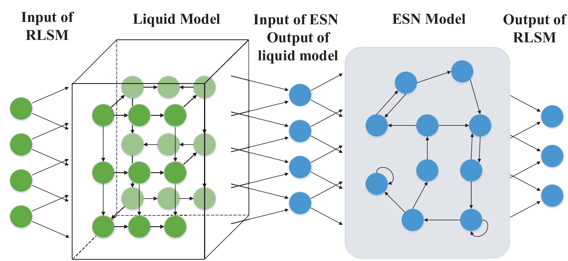
An ELSM based deep RL algorithm consists of eight components: a) agents, b) input of ELSM, c) liquid model, d) output of liquid model, e) input of ESN, f) ESN model, and g) output of ELSM, as shown in Fig. 3. For each SBS $j$, the components of deep RL using ELSM are specifically defined as follows:

• •

  Agents: The agents that implement the ELSM algorithm are the SBSs. Each SBS implements one ELSM algorithm for maximizing the reliability of its associated users.

• •

  Input of ELSM: The input of the ELSM deep RL algorithm is a vector $\boldsymbol{x}_{\tau,j}=\left[{x_{\tau,j1},\cdots,x_{\tau,jB}}\right]^{\mathrm{T}}$ where $x_{\tau,jk}$ represents the index of the policy that SBS $k$ uses for action selection at a period $\tau$ consisting of $N_{\tau}$ time slots. $\boldsymbol{x}_{\tau,j}$ is then used to estimate the ELSM output that captures the total reliability of the users associated with SBS $j$.

• •

  Liquid Model: The liquid model for each SBS is used to store the ELSM input information. Then, an ESN can use the historical input information to estimate the the users’ reliability. The liquid model consists of $N_{L}=L_{1}\times L_{2}\times L_{3}$ leaky integrate and fire neurons [24] that are arranged in a three dimensional-column.

  The liquid model typically has two categories of neurons: inhibitory neurons and excitatory neurons. An excitatory neuron will increase the information of the neurons in the next layer while an inhibitory neuron will decrease the information of the neurons in the next layer. The information state of each neuron $n$ at each time slot $t$ is ${v_{jn}}\left(t\right)$, which can be calculated using [15, Equation (13)]. The connections from the ELSM input to the liquid model are made with probability ${P}_{\textrm{IN}}$. The probability of having a connection between neurons $i$ and $j$ in the liquid model can be given by ${{P}_{ij}}=\varsigma{e^{-{{\left({{\zeta_{ij}\mathord{\left/{\vphantom{{\zeta}\lambda}}\right.\kern-1.2pt}\lambda}}\right)}^{2}}}}$, where $\varsigma\in\left\{{{\varsigma_{\textrm{EE}}},{\varsigma_{\textrm{EI}}},{\varsigma_{\textrm{IE}}},{\varsigma_{\textrm{II}}}}\right\}$ is a constant that depends on the type of both neurons. In particular, $\varsigma_{\textrm{EE}}$ denotes an excitatory-excitatory connection, $\varsigma_{\textrm{EI}}$ is an excitatory-inhibitory connection, $\varsigma_{\textrm{IE}}$ is an inhibitory-excitatory connection, and $\varsigma_{\textrm{II}}$ is a inhibitory-inhibitory connection. $\zeta_{ij}$ is the Euclidean distance between neurons $i$ and $j$. $\lambda$ influences how often neurons are connected.

• •

  Output of Liquid Model (Input of ESN): The output of the liquid model at period $\tau$ is a vector $\boldsymbol{\varphi}_{j}\!\left(\tau\right)\!=\!\left[{{\boldsymbol{v}_{j}}\!\left(1\right);\ldots;\boldsymbol{v}_{j}}\!\left(N_{\tau}\right)\right]$ where $\boldsymbol{\varphi}_{j}\left(t\right)\in{\mathbb{R}^{N_{\tau}N_{L}\times 1}}$ and $\boldsymbol{v}_{j}\left(t\right)=\left[{{v_{j1}}\left(t\right),\ldots,{v_{{jN_{L}}}}\!\left(t\right)}\right]$ with ${v_{jn}}\left(t\right)$ being the information state of neuron $n$ at time slot $t$. In fact, the ELSM uses unique output of liquid model to represent each input information. We can also see that the size of the input vector is $B$ while the size of the output vector is $N_{\tau}N_{L}$. This implies that the liquid model can use its spiking neurons to extract and extend the dynamics of the input information. As shown in Fig. 3, since the ESN is connected to the liquid model, the input of the ESN is essentially the output of liquid model.

• •

  ESN Model: The ESN model is used to find the relationship between the input and output of the ESN. The ESN model consists of an input matrix $\boldsymbol{W}_{j}^{\textrm{in}}\in\mathbb{R}^{N_{W}\times N_{L}N_{\tau}}$, a recurrent matrix $\boldsymbol{W}_{j}\in\mathbb{R}^{N_{W}\times N_{W}}$ , and an output weight matrix $\boldsymbol{W}_{j}^{\textrm{out}}\in\mathbb{R}^{N_{O}\times\left(N_{W}+N_{L}N_{\tau}\right)}$. Here, $N_{W}$ represents the number of neurons in ESN model and $N_{O}$ is the number of actions of the ELSM algorithm.

• •

  Action: Each action $i$ of the ELSM algorithm implemented by SBS $j$ is a vector $\boldsymbol{o}_{ji}\left(t\right)\!=\!\left[{\boldsymbol{u}_{ji}}\left(t\right);\boldsymbol{q}_{ji}\left(t\right)\right]$ where ${\boldsymbol{u}_{ji}}\left(t\right)\!=\!\left[{{u}_{ji1}}\left(t\right),\ldots,{{u}_{jiN_{U_{j}}}}\left(t\right)\right]$ with ${{u}_{jik}}\left(t\right)\in\left\{0,1\right\}$. ${{u}_{jik}}\!=\!1$ implies that, under action $i$, user $k$ will be associated with SBS $j$, and ${{u}_{jik}}=0$, otherwise. $\boldsymbol{q}_{ji}\left(t\right)=\left[q_{ji1}\left(t\right),\ldots,q_{jiN}\left(t\right)\right]$ where $q_{jik}\in\left\{0,120^{\circ},360^{\circ}\right\}$. $q_{jik}=0$ implies that when SBS $j$ uses action $i$, content $k$ is not stored in the cache while $q_{jik}=120^{\circ}$ ($q_{jik}=360^{\circ}$) implies that SBS $j$ stores visible ($360^{\circ}$) content $k$. In fact, action $\boldsymbol{o}_{ji}\left(t\right)$ determines the user association policy and cached contents at time $t$. We can also define an alternative action $\boldsymbol{o}_{ji}^{\prime}\left(t\right)=\left[{\boldsymbol{u}_{ji}}\left(t\right);\boldsymbol{z}_{ji}\left(t\right)\right]$ that determines the user association policy and content transmission format. Here, $\boldsymbol{z}_{ji}\left(t\right)=\left[z_{ji1}\left(t\right),\ldots,z_{jiN}\left(t\right)\right]$ where $z_{jik}\in\left\{120^{\circ},360^{\circ}\right\}$. $z_{jik}=120^{\circ}$ implies that the UAVs will transmit visible content $a$ to user $i$ while $z_{jik}=360^{\circ}$ implies that the UAVs will transmit $360^{\circ}$ content $a$ to user $i$. In fact, action $\boldsymbol{o}_{ji}\left(t\right)$ determines the user association policy and cached contents. Meanwhile, action $\boldsymbol{o}_{ji}^{\prime}\left(t\right)$ decides the user association and transmission content format. The SBSs will determine the use of either $\boldsymbol{o}_{ji}\left(t\right)$ or $\boldsymbol{o}_{ji}^{\prime}\left(t\right)$ according to the cache storage size, the number of users, and the number of UAV contents. Note that, for each implementation of the ELSM algorithm, each SBS will can at most use one action ($\boldsymbol{o}_{ji}\left(t\right)$ or $\boldsymbol{o}_{ji}^{\prime}\left(t\right)$).

• •

  Output of ELSM (output of ESN): For each action $i$ that SBS $j$ takes, the ELSM algorithm will output the estimated total reliability for users associated with SBS $j$. Thus, the output of the ELSM algorithm is ${{y}_{j}\!\left(\boldsymbol{o}_{ji}\!\left(t\right)\!\right)}\!=\!\sum\limits_{i\in\mathcal{U}_{j}}\!\!{\bar{\mathbbm{P}}_{i}}\!\left(\boldsymbol{o}_{ji}\left(t\right)\right)$. If the SBS use action $\boldsymbol{o}_{ji}^{\prime}\left(t\right)$, then the output of the ELSM is ${{y}_{j}\left(\boldsymbol{o}_{ji}^{\prime}\left(t\right)\right)}=\sum\limits_{i\in\mathcal{U}_{j}}{\bar{\mathbbm{P}}_{i}}\!\left(\boldsymbol{o}_{ji}^{\prime}\left(t\right)\right)$.

To allow the ELSM algorithm to estimate the users’ reliability, we need to calculate the successful transmission of users when SBS $j$ uses action $\boldsymbol{o}_{ji}\left(t\right)$ at time $t$. A transmission is said to be successful if the total processing and transmission delays of each user meet the delay requirements. The number of users that have successful transmission can be derived by the following theorem.

From Theorem 1, we can see that the content transmission format depends on the data rates of backhaul and users, the computational resources of each UAV and SBS, the content size, and the number of users that request the same content. From Theorem 1, we can also see that, as the number of users that request the same content increases, it will be better for the UAVs to transmit $360^{\circ}$ contents to the SBSs.

If each SBS $j$ uses action $\boldsymbol{o}_{ji}^{\prime}\left(t\right)$ for the implementation of the ELSM algorithm, the number of users that have successful transmissions at time $t$, which is given by the following theorem.

From Theorem 2, we can see that the cached contents of each SBS $j$ depend on the data rates of backhaul and users, the number of users associated with SBS $j$, the computational resources allocated to each user, and the cache storage size. Theorem 2 shows that, if the cache storage size is unlimited, storing each visible content for each user is better than storing a $360^{\circ}$ content. This is due to the fact that an SBS that stores visible contents can directly send its cached visible contents to its users without performing any backhaul transmission or visible content extraction. When the cache storage is limited, the SBSs may store $360^{\circ}$ contents to save cache storage. This, in turn, will increase the processing delay. In consequence, the SBSs need to balance the tradeoff between saving cache storage and increasing processing delay. Based on Theorem 2, each SBS $j$ calculates the number of users that have successful transmission so as to calculate the users’ reliability.

Next, we explain how each SBS $j$ uses the ELSM algorithm to solve problem (14). We first introduce the policy that each SBS $j$ uses for action selection at each time slot $t$. Then, the use of ELSM algorithm for users’ reliability estimation is specified.

For the proposed algorithm, we only need to train the output weight matrix of ESN. In consequence, we can directly use the result of [17, Theorem 2] which has proved that, for each action $\boldsymbol{o}_{ji}$, ESNs will converge to $\sum\limits_{i\in\mathcal{U}_{j}}{{\mathbbm{P}}_{i}}\!\left(\boldsymbol{o}_{ji}\left(t\right)\right)$ where $\mathcal{A}_{-j}=\prod\nolimits_{k\neq j,k\in\mathcal{B}}{{\mathcal{A}_{k}}}$ is the set of actions other than the action of SBS $j$. To improve the value of $\sum\limits_{i\in\mathcal{U}_{j}}{{\mathbbm{P}}_{i}}\!\left(\boldsymbol{o}_{ji}\left(t\right)\right)$, the ELSM algorithm uses Boltzmann policy for action selection instead of the work in [17] that uses a greedy mechanism. We assume that the users’ reliability resulting from the ELSM algorithm that uses a Boltzmann policy or a greedy mechanism for action selection are $\sum\limits_{i\in\mathcal{U}_{j}}{{\mathbbm{P}}_{i}}\!\left(\boldsymbol{o}_{j}\right)$ and $\sum\limits_{i\in\mathcal{U}_{j}}{{\mathbbm{P}}_{i}^{\varepsilon}}\!\left(\boldsymbol{o}_{j}\right)$, respectively. Then the relationship between $\sum\limits_{i\in\mathcal{U}_{j}}{{\mathbbm{P}}_{i}}\!\left(\boldsymbol{o}_{j}\right)$ and $\sum\limits_{i\in\mathcal{U}_{j}}{{\mathbbm{P}}_{i}^{\varepsilon}}\!\left(\boldsymbol{o}_{j}\right)$ can be given by the following theorem.

From Theorem 3, we can see that the value at the convergence point stemming from the proposed algorithm depends on the action selection policy used by the learning algorithm. As $\kappa$ in (16) increases, the proposed algorithm will use more iterations for exploration and the number of iterations for exploitation decreases. Hence, the system performance will decrease and the convergence speed increases. As $\kappa$ decreases, the proposed learning algorithm will use more iterations for exploitation and less iterations for exploration, and, then, system performance (i.e., reliability) will increase while the convergence speed decreases. In consequence, we need to appropriately adjust $\kappa$ to balance the exploration and exploitation so as to balance the convergence speed and the reliability that the proposed algorithm can achieve.

To calculate the number of users that have successful transmissions, we need to simplify the problem in (14). Given a vector $\boldsymbol{o}_{ji}\left(t\right)$, (14) can be simplified as:

References

- [1] E. Bastug, M. Bennis, M. Medard, and M. Debbah, “Toward interconnected virtual reality: Opportunities, challenges, and enablers,” IEEE Communications Magazine, vol. 55, no. 6, pp. 110–117, June 2017.
- [2] K. Hamidouche, W. Saad, M. Debbah, J. B. Song, and C. S. Hong, “The 5G cellular backhaul management dilemma: To cache or to serve,” IEEE Transactions on Wireless Communications, vol. 16, no. 8, pp. 4866–4879, Aug 2017.
- [3] G. Schaufler and W. Stürzlinger, “A three dimensional image cache for virtual reality,” Computer Graphics Forum, vol. 15, no. 3, pp. 227–235, Aug. 1996.
- [4] J. Chakareski, “VR/AR immersive communication: Caching, edge computing, and transmission trade-offs,” in Pro. of the Workshop on Virtual Reality and Augmented Reality Network, Los Angeles, CA, USA, Aug. 2017.
- [5] T. X. Tran, F. Kazemi, E. Karimi, and D. Pompili, “Mobee: Mobility-aware energy-efficient coded caching in cloud radio access networks,” in Proc. of IEEE International Conference on Mobile Ad Hoc and Sensor Systems (MASS), Orlando, FL, USA, Oct 2017.
- [6] N. Zhao, F. Cheng, F. R. Yu, J. Tang, Y. Chen, G. Gui, and H. Sari, “Caching UAV assisted secure transmission in hyper-dense networks based on interference alignment,” IEEE Transactions on Communications, to appear, 2018.
- [7] M. Chen, M. Mozaffari, W. Saad, C. Yin, M. Debbah, and C. S. Hong, “Caching in the sky: Proactive deployment of cache-enabled unmanned aerial vehicles for optimized quality-of-experience,” IEEE Journal on Selected Areas in Communications, vol. 35, no. 5, pp. 1046–1061, May 2017.
- [8] M. Hajimirsadeghi, N. B. Mandayam, and A. Reznik, “Joint caching and pricing strategies for popular content in information centric networks,” IEEE Journal on Selected Areas in Communications, vol. 35, no. 3, pp. 654–667, March 2017.
- [9] X. Xu, Y. Zeng, Y. L. Guan, and R. Zhang, “Overcoming endurance issue: UAV-enabled communications with proactive caching,” available online: arxiv.org/abs/1712.03542, Dec. 2017.
- [10] O. Semiari, W. Saad, M. Bennis, and B. Maham, “Caching meets millimeter wave communications for enhanced mobility management in 5g networks,” IEEE Transactions on Wireless Communications, vol. 17, no. 2, pp. 779–793, Feb 2018.
- [11] J. Kwak, Y. Kim, L. B. Le, and S. Chong, “Hybrid content caching in 5G wireless networks: Cloud versus edge caching,” IEEE Transactions on Wireless Communications, to appear, 2018.
- [12] M. Mozaffari, W. Saad, M. Bennis, Y. H. Nam, and M. Debbah, “A tutorial on UAVs for wireless networks: Applications, challenges, and open problems,” available online: arxiv.org/abs/1803.00680, 2018.
- [13] Z. Zhao, M. Peng, Z. Ding, W. Wang, and H. V. Poor, “Cluster content caching: An energy-efficient approach to improve quality of service in cloud radio access networks,” IEEE Journal on Selected Areas in Communications, vol. 34, no. 5, pp. 1207–1221, May 2016.
- [14] Y. Dong, Md. Zoheb Hassan, J. Cheng, Md. J. Hossain, and V. C. M. Leung, “An edge computing empowered radio access network with UAV-mounted FSO fronthaul and backhaul: Key challenges and approaches,” IEEE Wireless Commun., to appear, 2018.
- [15] W. Maass, “Liquid state machines: Motivation, theory, and applications,” Computability in context: Computation and logic in the real world, pp. 275–296, 2010.
- [16] R. Ali and T. Peter, “Minimum complexity echo state network,” IEEE Transactions on Neural Networks, vol. 22, no. 1, pp. 131–144, November 2011.
- [17] M. Chen, W. Saad, and C. Yin, “Echo state networks for self-organizing resource allocation in LTE-U with uplink-downlink decoupling,” IEEE Transactions on Wireless Communications, vol. 16, no. 1, January 2017.
- [18] T. S. Rappaport, Wireless Communications: Principles and Practice, Upper Saddle River, NJ: Prentice-Hall, 2002.
- [19] T. S. Rappaport, F. Gutierrez, E. Ben-Dor, J. N. Murdock, Y. Qiao, and J. I. Tamir, “Broadband millimeter-wave propagation measurements and models using adaptive-beam antennas for outdoor urban cellular communications,” IEEE Transactions on Antennas and Propagation, vol. 61, no. 4, pp. 1850–1859, 2013.
- [20] A. Al-Hourani, S. Kandeepan, and A. Jamalipour, “Modeling air-to-ground path loss for low altitude platforms in urban environments,” in Proc. of IEEE Global Communications Conference (GLOBECOM), Austin, TX, USA, December 2014.
- [21] O. Semiari, W. Saad, M. Bennis, and M. Debbah, “Integrated millimeter wave and sub-6 GHz wireless networks: A roadmap for ultra-reliable low-latency communications,” available online: arxiv.org/abs/1802.03837, Feb. 2018.
- [22] M. Mozaffari, W. Saad, M. Bennis, and M. Debbah, “Unmanned aerial vehicle with underlaid device-to-device communications: Performance and tradeoffs,” IEEE Transactions on Wireless Communications, vol. 15, no. 6, pp. 3949–3963, June 2016.
- [23] Y. Li, “Deep reinforcement learning: An overview,” available online: arxiv.org/abs/1701.07274, Sep. 2017.
- [24] M. Chen, U. Challita, W. Saad, C. Yin, and M. Debbah, “Machine learning for wireless networks with artificial intelligence: A tutorial on neural networks,” available online: arxiv.org/abs/1710.02913, Oct. 2017.
- [25] M. Bennis and D. Niyato, “A Q-learning based approach to interference avoidance in self-organized femtocell networks,” in Proc. of IEEE Global Commun. Conference (GLOBECOM) Workshop on Femtocell Networks, Miami, FL, USA, Dec. 2010.