Prompt Scheduling for Selfish Agents

For one machine, weighted jobs, available at time zero, ordering the jobs in order of weight/processing time minimizes the sum of competition times Smith [1956]. For one machine, unweighted jobs with release times, a preemptive schedule that always processes the job with the minimal remaining processing time minimizes the sum of weighted completion times Schrage and Miller [1966]; Schrage [1968]. As an offline problem, where jobs cannot be executed prior to some earliest time, finding an optimal non-preemptive schedule is computationally hard Hall et al. [1997].

For parallel machines, where jobs arrive over time, a preemptive schedule that always processes the jobs with the highest priority: weight divided by remaining processing time, is a 2 approximation Megow and Schulz [2004], this algorithm is called weighted shortest remaining processing time (WSRPT). If all weights are one this preemptive algorithm is called shortest remaining processing time (SRPT). Other online and offline algorithms to minimize the sum of completion times appear in Bruno et al. [1974]; Shmoys et al. [1995]; Hall et al. [1997].

Phillips et al. [1998] show how to convert a preemptive online algorithm into a non-preemptive online algorithm while increasing the completion time of the job by no more than a constant factor. This transformation strongly depends on not determining immediately when the job will be executed. This is in comparison to a prompt algorithm that determines when the job is executed immediately upon the job arrival.

When selfish agents are involved, it is valuable to keep things simple Hartline and Roughgarden [2009]. Offering selfish agents an anonymous menu of options is an example of such a simple process. More complicated mechanisms require trust on the part of the agents.

Recently, Feldman et al. [2017] considered a similar question to ours, where a job with private processing time had to choose between multiple FIFO queues, where the servers had different speeds. Here, dynamic posted prices were associated with every queue, with the goal of [approximately] minimizing the makespan, the length of time until the last job would finish. Shortly thereafter, Im et al. [2017] used dynamic pricing to minimize the maximal flow time. Dynamic pricing schemes were considered for non-scheduling cost minimization problems in Cohen et al. [2015].

A constant approximation mechanism for minimizing sum of completion times for selfish jobs was considered in Gkatzelis et al. [2017], where the setting was an offline setting, the processing time was known in advance and the weight was private information. In an online setting, Im and Kulkarni [2016] show a constant approximation preemptive mechanism that gives an $O(1/\epsilon^{2})$ approximation to the sum of flow times when using machines that are faster by a factor of $1+\epsilon$.

In this paper our goals are pricing schemes that affect agents as to behave in a manner that [approximately] minimizes the sum of weighted completion times.

There is a vast body of work on machine scheduling problems, in offline and online settings, with strategic agents involved and not, and in a host of models. It is impossible to do justice to this body of work but a very short list of additional relevant papers includes Graham [1966]; Lenstra et al. [1977]; Graham et al. [1979]; Lenstra et al. [1990]; Nisan and Ronen [2001]; Christodoulou et al. [2004]; Immorlica et al. [2009].

If jobs have weight one, we give (optimal) menus that do not require pricing menu entries. Any entry on the menu is available for free. Therefore, we can simplify the menu structure as follows: The job chooses a time interval and a machine from a menu with entries of the form $([b,e],1\leq q\leq m)$ where the first entry is a time interval, and the second entry is a machine²² 2 Although the general setting allows pricing menu items, it turns out that for weight 1 jobs the optimal menu does not need to differentiate entries by price.. The crux of the matter is coming up with the right menu.

Jobs choose from the menu one of the entries immediately upon arrival. As above, we say that job $j$ chooses menu entry $(I(j),M(j))$ where $I(j)$ is an interval, and $1\leq M(j)\leq m$.

For job $j$ with arrival time $r_{j}$, and processing time $p_{j}$ the cost associated with choosing the menu item $([b,e],1\leq q\leq m)$ is $\infty$ if $p_{j}>e-b$ and $(b+p_{j})$ otherwise. Jobs always seek to minimize their cost.

Every job requires one unit of processing time on one of $m$ different processors. Every job $j$ is a selfish agent that has a private weight $w_{j}$, the cost to the job of one unit of delay.

The job chooses a machine and time slot from a menu with entries of the form $([i,i+1],1\leq q\leq m,\pi)$ where the first entry is a time slot, the second entry is a machine, and the third entry is the price of this time slot on the machine.

Jobs choose from the menu one of the entries immediately upon arrival. Job $j$ is said to choose menu item $(I(j),M(j),\Pi(j))$ where $I(j)$ is a length one interval, $1\leq M(j)\leq m$, and $\Pi(j)$ is the price to be paid for choosing this option.

For job $j$ with arrival time $r_{j}$, and weight $w_{j}$ the cost associated with choosing the menu item $([i,i+1],1\leq q\leq m,\pi)$ is $w_{j}(i+1)+\pi$. Jobs always seek to minimize their cost.

We present two natural algorithms for prompt scheduling on a single machine, which result in poor competitive ratios. Assume $P_{\max}=2^{d}$, for some constant $d$, and $P_{\max}$ is known in advance. Assume also that all jobs have release time $0$ (but arrive sequentially). In this case, the optimal algorithm sorts jobs from short to long processing times, and schedules them based on this order. In an attempt to mimic this optimal (offline) algorithm by an online algorithm — in case where the input starts with a sequence of long jobs — we would like to introduce delays, keeping some early intervals vacant for short jobs that might come in the future.

Consider an algorithm that sets a static interval sequence (i.e., a sequence that is set once and for all from the outset), and schedules each arriving job on the first interval on which it fits.

One natural algorithm sets (an infinite loop of) the following sequence of intervals: the $i$th interval for $i=0,\ldots,d$ is of length $2^{i}$.

Consider the following input: for $i=0,\ldots,d$, a job of size $2^{i}$ arrives (all jobs with release time zero, job $i+1$ follows job $i$), followed by $n$ jobs of length $1$ (where $n$ is determined later). The cost for the optimal algorithm is:

In the proposed algorithm, the last $n$ unit-length jobs will be scheduled after the first $d+1$ jobs, which have total processing time of $2^{d+1}-1$. This implies:

For $n=\Theta(2^{\nicefrac{{d}}{{2}}})$, we get that $Cost(OPT)=\Theta(2^{d})$, while $Cost(ALG)=\Omega\left(2^{d+\nicefrac{{d}}{{2}}}\right)$, leading to a competitive ratio of $\Omega\left(\sqrt{P_{\max}}\right)$.

The proposed algorithm failed because it did not leave enough space for the unit length jobs. A possible attempt to fix this problem would be to have more short intervals than long ones. One natural such sequence is (an infinite loop of) $2^{d}$ length 1 intervals, followed by $2^{d-1}$ length 2 intervals, etc., ending with a single interval of length $2^{d}$.

Consider an input sequence in which $2^{\nicefrac{{d}}{{2}}}$ jobs of size 2 arrive at time 0, followed by one large job of size $2^{d}$. The optimal schedule processes the short jobs first, then the large one, resulting in cost:

In the proposed algorithm, every short job will be scheduled after the first $2^{d}$ unit length intervals (as they do not fit unit length intervals). The obtained cost is thus

resulting in $\Omega\left(\sqrt{P_{\max}}\right)$ competitive ratio, as before. Thus, saving too much space for short jobs might result in unnecessary delay, which may lead to a poor competitive ratio.

Motivated by the above two failed attempts, we now present our solution:

We define sequences of integers $S_{k}$, $k=0,1,\ldots$, as follows: Let $S_{0}=\langle 1\rangle$ and for $k>0$ let $S_{k}=S_{k-1}\|S_{k-1}\|\langle 2^{k}\rangle$ where $\|$ denotes concatenation. Ergo,

Let $n_{k}=2^{k+1}-1$ denote the length of $S_{k}$ (follows inductively from $n_{0}=1$ and $n_{k}=2n_{k-1}+1$). Let $S_{k}[i]$, $i=1,\ldots,n_{k}$ be the $i$th element of $S_{k}$. Let $S_{\infty}$ be an infinite sequence whose length $n_{k}$ prefix is $S_{k}$ (for all $k$):

Let $S_{\infty}[i]$, $i=1,2,\ldots$ be the $i$th element of $S_{\infty}$. Note that $S_{k}[i]=S_{k^{\prime}}[i]$ for all $k\leq k^{\prime}$ and all $i=1,\ldots,n_{k}$, ergo, $S_{k}$ is a prefix of $S_{k^{\prime}}$ for $k\leq k^{\prime}$.

We use the $S_{k}$ sequences to define interval sequences. Let $\gamma_{i}$ be the sum of the first $i$ entries in $S_{\infty}$, $\gamma_{i}=\sum_{j=1}^{i}S_{\infty}[j]$ (i.e., $\gamma_{1}=1$, $\gamma_{2}=2$, $\gamma_{3}=4$, etc.).

We define $S_{k}(t)$, $t\geq 0$, to be a sequence of $n_{k}$ consecutive intervals, the first of which starts at time $t$, and where the length of the $j$th interval equals $S_{k}[j]$. I.e.,

For example

For any interval sequence $S$ let $b(S)$ be the start of the first interval in $S$ and let $e(S)$ be the end of the last interval in $S$. For example, $b(S_{2}(2))=2$ and $e(S_{2}(2))=14$.

We say that $S_{k}$ appears in $S_{d}(t)$ if there exists some $t^{\prime}$ such that the interval sequence $S_{k}(t^{\prime})$ is a contiguous subsequence of $S_{d}(t)$. In this case we also say that $S_{k}(t^{\prime})$ appears in $S_{d}(t)$. Note that while $S_{k}$ is a sequence of integers, both $S_{k}(t^{\prime})$ and $S_{d}(t)$ are interval sequences.

By construction, for any $k$ and any $t\neq t^{\prime}$ if $S_{k}(t)$ and $S_{k}(t^{\prime})$ appear in some $S_{d}(\tilde{t})$, then $\left[b(S_{k}(t)),e(S_{k}(t))\right]$ and $\left[b(S_{k}(t^{\prime})),e(S_{k}(t^{\prime}))\right]$ are disjoint except, possibly, for their endpoints. Let $I$ be an interval of length $2^{k}$ that appears in $S_{\infty}(t)$. Then there is a unique $t^{\prime}$ such that $S_{k}(t^{\prime})$ appears in $S_{\infty}(t)$ and $I$ is the last interval of $S_{k}(t^{\prime})$. It follows from Lemma 1 that

The interval sequences defined above suggests a new possible static algorithm. Divide the timeline of each machine into intervals as in $S_{\infty}(0)$, and let any job that arrives occupy the first unoccupied interval it fits in. Unfortunately, as proved in section B, when the competitive ratio is evaluated as a function of $P_{\max}$ alone, this algorithm is $\Omega\left(\sqrt{P_{\max}}\right)$ competitive, as the natural algorithms in Section 3.1. (When the competitive ratio may be a function of $P_{\max}$ and $n$, this algorithm is $O\left(\log P_{\max}+\log n\right)$ competitive, see Theorem 5).

When job $j+1$ arrives the algorithm is in some configuration $\psi^{j}=\left(A^{j},X^{j}\right)$, where $A^{j}$ is some state of length $\ell_{j}$, and $X^{j}$ is the set of intervals occupied by the previous $j$ jobs. State $A^{j}$ represents every machines’ division of $\left[0,\max_{i\in[j]}c_{i}\right]$ into time intervals (same division for all machines). This division will be kept at any future time. For every $i<\ell_{j}$, $A^{j}_{i}$ is fixed and will be a part of every future state, while $A^{j}_{\ell_{j}}$ might be subject to change. We refer to $A^{j}_{\ell_{j}}$ as the tentative sequence of state $A^{j}$. $X^{j}$ keeps track of all previously allocated intervals (in all machines): $([b,e],q)\in X^{j}$ means that some job $j^{\prime}<j$ chose the interval $[b,e]$ on machine $1\leq q\leq m$. Note that the size of job $j$, $p_{j}$, might be strictly smaller than the length of the interval ($e-b$), yet it is still considered occupied.

Given a state $A=\left(A_{1},A_{2},\ldots,A_{\ell}\right)$ and a time $t$, we define an interval sequence $\tau$ as follows:

$\tau$ is used to create the menu presented to a job $j$. We present an algorithm for the creation of the menu, based on the previous configuration $\psi^{j-1}$, and the current time $t$.
• Let $\tau^{j}=\tau\left(A^{j-1},r_{j}\right)$. • Set $d_{1}$ to be the length of the first time interval in $\tau^{j}$ beginning at time $b_{1}\geq t$. • Add $([b_{1},b_{1}+d_{1}],q)$ to the menu for all machines $1\leq q\leq m$ in which $[b_{1},b_{1}+d_{1}]$ is unoccupied (i.e, $([b_{1},b_{1}+d_{1}],q)\notin X^{j-1}$). • Set $i=1$ • Repeat until job $j$ chooses an interval: – Let $d_{i+1}$ be the length of the first interval longer than $d_{i}$ in $\tau^{j}$ that starts at time $b_{i+1}\geq t$ (it follows that $b_{i+1}>b_{i}$). – Add $([b_{i+1},b_{i+1}+d_{i+1}],q)$ to the menu for all machines $1\leq q\leq m$ in which $[b_{i+1},b_{i+1}+d_{i+1}]$ is unoccupied (i.e., $([b_{i+1},b_{i+1}+d_{i+1}],q)\notin X^{j-1}$). – Set $i=i+1$.

By construction, no job will ever choose a time interval that starts before the job arrival time, nor will it ever choose a slot that has already been chosen.

A selfish job of length $p_{j}$ always chooses a menu entry of the form $([b,e],q$) where $b$ is the earliest menu entry with $p_{j}\leq e-b$.

After job $j$ makes its choice of menu entry, $(I(j),M(j))$, we update the configuration from $\psi^{j-1}=\left(A^{j-1},X^{j-1}\right)$ to $\psi^{j}=\left(A^{j},X^{j}\right)$. Clearly, $X^{j}=X^{j-1}\cup\left\{(I(j),M(j))\right\}$. In the rest of this section we describe how to compute $A^{j}$.

Recall that a state is a vector of consecutive and disjoint interval sequences. Initially, $A^{0}=\langle\rangle$ with length $\ell_{0}=0$ and $A^{0}_{\ell_{0}}$ is an empty sequence with $b\left(A^{0}_{\ell_{0}}\right)=e\left(A^{0}_{\ell_{0}}\right)=0$. $A^{j}$ always contains all of $A^{j-1}$’s interval sequences except possibly the tentative sequence $A^{j-1}_{\ell_{j-1}}$. When job $j$ of size $2^{k}$ chooses an interval, the new tentative sequence $A^{j}_{\ell_{j}}$ can be one of the following:

1. 1.

   Unchanged from former: The new tentative sequence in $A^{j}$ is the same as the former tentative sequence in $A^{j-1}$, i.e., $A^{j}_{\ell_{j}}=A^{j-1}_{\ell_{j-1}}$. This happens when $I(j)\in A^{j-1}$, see entry $1$ in Table 2.

2. 2.

   Disjoint from former: The former tentative sequence, $A^{j-1}_{\ell_{j-1}}$ becomes fixed, and the new tentative sequence $A^{j}_{\ell_{j}}$ is disjoint from the former. The tentative sequence in $A^{j-1}$, $A^{j-1}_{\ell_{j-1}}$, is the $\ell_{j-1}$th element in all future states $A^{i}$, for $i\geq j$. See entries $2$ and $3$ in Table 2.

3. 3.

   Extension of former: The new tentative sequence is an extension of the former tentative sequence. I.e., if $A^{j-1}_{\ell_{j-1}}=S_{d}(t)$ then $\ell_{j}=\ell_{j-1}$ and $A^{j}_{\ell_{j}}=S_{k}(t)$. See entry $4$ in Table 2.

Let $A^{j}_{i},A^{j}_{i+1}$ be two consecutive interval sequences in a state $A^{j}$. If $b\left(A^{j}_{i+1}\right)>e\left(A^{j}_{i}\right)$, we say the interval $\left[e\left(A^{j}_{i}\right),b\left(A^{j}_{i+1}\right)\right]$ is a gap.

Figure 1 is an example with 5 jobs that arrive over time, and how the configuration changes over time. The jobs in Figure 1 illustrate cases 1–4 from Table 2 in the following order: case 2 for job 1, case 1 for job 2, case 3 for job 3, case 4 for job 4 and case 2 for job 5.

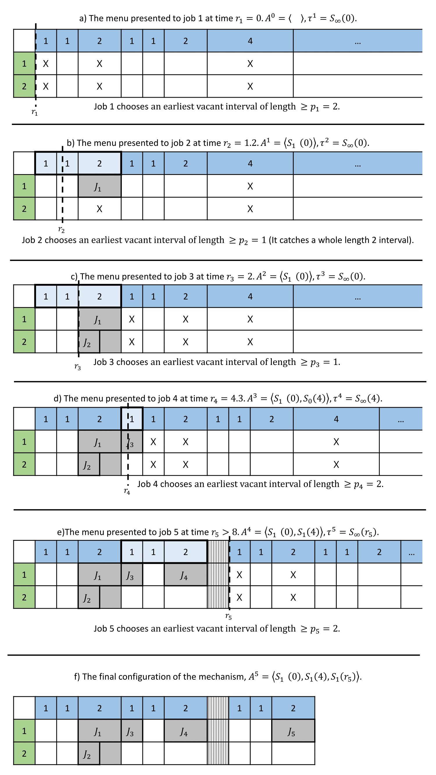
Based on the definition of $A^{j}$ and its update rule, we observe the following.

References

- Bruno et al. [1974] J. Bruno, E. G. Coffman, Jr., and R. Sethi. Scheduling independent tasks to reduce mean finishing time. Commun. ACM, 17(7):382–387, July 1974. ISSN 0001-0782. doi: 10.1145/361011.361064.
- Christodoulou et al. [2004] George Christodoulou, Elias Koutsoupias, and Akash Nanavati. Coordination mechanisms. In Automata, Languages and Programming: 31st International Colloquium, ICALP 2004, Turku, Finland, July 12-16, 2004. Proceedings, pages 345–357, 2004. doi: 10.1007/978-3-540-27836-8_31.
- Cohen et al. [2015] Ilan Reuven Cohen, Alon Eden, Amos Fiat, and Lukasz Jez. Pricing online decisions: Beyond auctions. In Proceedings of the Twenty-Sixth Annual ACM-SIAM Symposium on Discrete Algorithms, SODA 2015, San Diego, CA, USA, January 4-6, 2015, pages 73–91, 2015. doi: 10.1137/1.9781611973730.7.
- Daskalakis et al. [2017] Constantinos Daskalakis, Moshe Babaioff, and Hervé Moulin, editors. Proceedings of the 2017 ACM Conference on Economics and Computation, EC ’17, Cambridge, MA, USA, June 26-30, 2017, 2017. ACM. ISBN 978-1-4503-4527-9. doi: 10.1145/3033274.
- Feldman et al. [2017] Michal Feldman, Amos Fiat, and Alan Roytman. Makespan minimization via posted prices. In Daskalakis et al. [2017], pages 405–422. ISBN 978-1-4503-4527-9. doi: 10.1145/3033274.3085129.
- Gkatzelis et al. [2017] Vasilis Gkatzelis, Evangelos Markakis, and Tim Roughgarden. Deferred-acceptance auctions for multiple levels of service. In Daskalakis et al. [2017], pages 21–38. ISBN 978-1-4503-4527-9. doi: 10.1145/3033274.3085142.
- Graham [1966] R. L. Graham. Bounds for certain multiprocessing anomalies. Bell System Technical Journal, 45:1563–1581, 1966.
- Graham et al. [1979] Ronald L Graham, Eugene L Lawler, Jan Karel Lenstra, and AHG Rinnooy Kan. Optimization and approximation in deterministic sequencing and scheduling: a survey. In Annals of discrete mathematics, volume 5, pages 287–326. Elsevier, 1979.
- Hall et al. [1997] Leslie A. Hall, Andreas S. Schulz, David B. Shmoys, and Joel Wein. Scheduling to minimize average completion time: Off-line and on-line approximation algorithms. Math. Oper. Res., 22(3):513–544, 1997. doi: 10.1287/moor.22.3.513.
- Hartline and Roughgarden [2009] Jason D. Hartline and Tim Roughgarden. Simple versus optimal mechanisms. In Proceedings 10th ACM Conference on Electronic Commerce (EC-2009), Stanford, California, USA, July 6–10, 2009, pages 225–234, 2009. doi: 10.1145/1566374.1566407.
- Im and Kulkarni [2016] Sungjin Im and Janardhan Kulkarni. Fair online scheduling for selfish jobs on heterogeneous machines. In Proceedings of the 28th ACM Symposium on Parallelism in Algorithms and Architectures, SPAA 2016, Asilomar State Beach/Pacific Grove, CA, USA, July 11-13, 2016, pages 185–194, 2016. doi: 10.1145/2935764.2935773.
- Im et al. [2017] Sungjin Im, Benjamin Moseley, Kirk Pruhs, and Clifford Stein. Minimizing maximum flow time on related machines via dynamic posted pricing. In Kirk Pruhs and Christian Sohler, editors, 25th Annual European Symposium on Algorithms, ESA 2017, September 4-6, 2017, Vienna, Austria, volume 87 of LIPIcs, pages 51:1–51:10. Schloss Dagstuhl - Leibniz-Zentrum fuer Informatik, 2017. ISBN 978-3-95977-049-1. doi: 10.4230/LIPIcs.ESA.2017.51.
- Immorlica et al. [2009] Nicole Immorlica, Li (Erran) Li, Vahab S. Mirrokni, and Andreas S. Schulz. Coordination mechanisms for selfish scheduling. Theor. Comput. Sci., 410(17):1589–1598, 2009. doi: 10.1016/j.tcs.2008.12.032.
- Lenstra et al. [1990] Jan Karel Lenstra, David B. Shmoys, and Éva Tardos. Approximation algorithms for scheduling unrelated parallel machines. Math. Program., 46:259–271, 1990. doi: 10.1007/BF01585745.
- Lenstra et al. [1977] J.K. Lenstra, A.H.G. Rinnooy Kan, and P. Brucker. Complexity of machine scheduling problems. In P.L. Hammer, E.L. Johnson, B.H. Korte, and G.L. Nemhauser, editors, Studies in Integer Programming, volume 1 of Annals of Discrete Mathematics, pages 343 – 362. Elsevier, 1977. doi: https://doi.org/10.1016/S0167-5060(08)70743-X.
- Megow and Schulz [2004] Nicole Megow and Andreas S. Schulz. On-line scheduling to minimize average completion time revisited. Oper. Res. Lett., 32(5):485–490, 2004. doi: 10.1016/j.orl.2003.11.008.
- Nisan and Ronen [2001] Noam Nisan and Amir Ronen. Algorithmic mechanism design. Games and Economic Behavior, 35(1-2):166–196, 2001.
- Phillips et al. [1998] Cynthia Phillips, Clifford Stein, and Joel Wein. Minimizing average completion time in the presence of release dates. Mathematical Programming, 82(1):199–223, Jun 1998. ISSN 1436-4646. doi: 10.1007/BF01585872.
- Schrage [1968] Linus Schrage. Letter to the editor-a proof of the optimality of the shortest remaining processing time discipline. Operations Research, 16(3):687–690, 1968.
- Schrage and Miller [1966] Linus E. Schrage and Louis W. Miller. The queue m / g /1 with the shortest remaining processing time discipline. Operations Research, 14(4):670–684, 1966.
- Shmoys et al. [1995] David B. Shmoys, Joel Wein, and David P. Williamson. Scheduling parallel machines on-line. SIAM J. Comput., 24(6):1313–1331, 1995. doi: 10.1137/S0097539793248317.
- Smith [1956] Wayne E. Smith. Various optimizers for single-stage production. Naval Research Logistics Quarterly, 3(1-2):59–66, 1956. ISSN 1931-9193. doi: 10.1002/nav.3800030106.
Appendix A The Static Mechanism Upper Bound
In this section, we analyze a mechanism based on a single component of Section 3. We divide the timeline interval into time intervals as in , in every machine. This division does not change over time, i.e., this is a static mechanism. Upon arrival, a job may choose an unoccupied interval in in some machine. Denote this mechanism as ALG.
Let be a sequence of jobs. Let be the maximal processing time among all jobs. Recall that we may assume that all jobs processing time are of length for some . Therefore, there are at most different processing times for jobs in . Let for . Let . We prove our static mechanism achieves the following competitive ratio:
Theorem 5.
The competitive ratio of ALG is
Proof.
Let be the completion time of job in SRPT. We prove that for every job ,
Let be a job in the input sequence with .
- •
If is assigned in for some machine (i.e., in the first slot in that machine), then by Corollary 1 , while . . Therefore,
Otherwise, as , there exists some with . Let be such that . Notice that as did not choose the first interval. We look at two possible cases:
- –
. In this case by Corollary 1 while . Thus,
. Then for every machine, all intervals of size that are in are occupied. By Corollary 1 there are different appearances of in . There are at most appearances of in (only if ). Using Lemma 2 on every such appearance on every machine separately, suggests that
(as ), i.e., the total volume of jobs no greater than on every machine in that arrived no later then job , is at least . Ergo, there is an overall total volume of .
As there are different processing times possible for jobs with processing time , we get that . In SRPT, job will be scheduled after a volume of at least scattered among machines, therefore . Thus,
∎
Appendix B A Lower Bound for the Static Mechanism
In this section we show that, as a function of (without ), and with jobs feedback (i.e., a job does not occupy an entire interval if it is larger than the job size) the competitive ratio of the static mechanism is .
Consider the following input for some fixed with :
•
First, jobs with processing time arrive one after the other (at time 0).
Set .
While :
–
jobs with processing time arrive one after the other (at time 0).
Set
Finally, jobs with processing time 1 arrive one after the other (at time 0)
The input described may be described as follows - at first we fill all intervals in with jobs of size at most . We fill every interval of length with jobs of size ( jobs for interval of length ). Recall that the sum of the length of intervals in equals (Corollary 1), and that for every the total length of intervals of length in is . It follows that the total length of intervals of lengths in is . We then fill every interval for with a job of processing time . After all intervals in are occupied, we add jobs with processing time 1.
The last jobs are all completed (and start) later than . Thus, . The optimal algorithm, SPT schedules the jobs by increasing order of their sizes. We denote the cost induced by all jobs of size by . The cost of a single job of size is the total processing time of all smaller jobs plus the total processing time of sized jobs that arrived before it, i.e, the completion time of the th job of size is . This implies the following cost function:
For we get that while and . Thus, the competitive ratio is .