Set Similarity Search for Skewed Data11footnotetext: The research leading to these results has received funding from the European Research Council under the European Union’s 7th Framework Programme (FP7/2007-2013) / ERC grant agreement no. 614331. BARC, Basic Algorithms Research Copenhagen, is supported by the VILLUM Foundation grant 16582.
Abstract
Set similarity join, as well as the corresponding indexing problem set similarity search, are fundamental primitives for managing noisy or uncertain data. For example, these primitives can be used in data cleaning to identify different representations of the same object. In many cases one can represent an object as a sparse 0-1 vector, or equivalently as the set of nonzero entries in such a vector. A set similarity join can then be used to identify those pairs that have an exceptionally large dot product (or intersection, when viewed as sets). We choose to focus on identifying vectors with large Pearson correlation, but results extend to other similarity measures. In particular, we consider the indexing problem of identifying correlated vectors in a set of vectors sampled from . Given a query vector and a parameter , we need to search for an -correlated vector in a data structure representing the vectors of . This kind of similarity search has been intensely studied in worst-case (non-random data) settings.
Existing theoretically well-founded methods for set similarity search are often inferior to heuristics that take advantage of skew in the data distribution, i.e., widely differing frequencies of 1s across the dimensions. The main contribution of this paper is to analyze the set similarity problem under a random data model that reflects the kind of skewed data distributions seen in practice, allowing theoretical results much stronger than what is possible in worst-case settings. Our indexing data structure is a recursive, data-dependent partitioning of vectors inspired by recent advances in set similarity search. Previous data-dependent methods do not seem to allow us to exploit skew in item frequencies, so we believe that our work sheds further light on the power of data dependence.
1 Introduction
Data management is increasingly moving from a world of well-ordered, curated data sets to settings where data may be noisy, incomplete, or uncertain. This requires primitives that are able to work with notions of “approximate match”, as opposed to the exact matches used in standard hash indexes and in equi-joins. Such functionality is particularly challenging to scale when data is high-dimensional, informally because of the curse of dimensionality which makes it hard to organize data in such a way that approximate matches can be efficiently identified. In this paper we consider the fundamental primitive set similarity join and more specifically the indexing problem set similarity search. A set similarity join is used to identify pairs of sets that are similar in the sense that they have an “exceptionally large intersection”. Many notions of “exceptionally large intersection” exist, but from a theoretical point of view they are essentially equivalent [18]. We will consider the encoding of sets as sparse 0-1 vectors, and use Pearson correlation as the measure of similarity; we give more details below.
The information retrieval and database communities have extensively worked on designing scalable algorithms for similarity join, see e.g. the recent book by Augsten and Böhlen [10]. The state-of-the-art for practical set similarity join algorithms is reflected in the recent mini-survey and comprehensive empirical evaluation of Mann et al. [31]. The best methods in practice are ones that exploit the significant skew in frequencies of set elements that exists in many data sets. When there is insufficient skew these methods become inefficient, and in the worst case they degenerate to a trivial brute-force algorithm. In contrast, strong theoretical results are known when randomization and approximation of distances is allowed, e.g. [2, 18, 22, 25, 46]. Even though existing randomized algorithms for set similarity search are superior to commonly used heuristics for difficult data distributions with small skew, it is clear that the heuristics will work much better (in theory and in practice) when the skew is large enough.
In this paper we target this disconnect between theory and practice, presenting a new data structure that, in a certain way, can interpolate between the best existing methods for small skew and heuristics that work well with large skew. Our message is that modeling skew can lead to algorithms that takes advantage of structure in data in a way that is theoretically justified. This complements recent advances in the theory of data dependent methods for high-dimensional search, where clustering structure in data (rather than skew) is exploited to achieve faster algorithms, even in the worst case [6, 8].
Motivating example.
Suppose we wish to search -dimensional boolean vectors chosen from the “harmonic” distribution where the th bit is set with probability , independently for each and each . The boolean vectors represent subsets of . For consistency with the rest of the paper, we refer to these elements as vectors, but use some set notation for simplicity; i.e. is used to represent the Hamming weight of .
Assuming (for now) , all vectors have Hamming weight close to the expectation with high probability by Chernoff bounds. We wish to search for a vector that is correlated with a query vector such that , for some parameter .
Define to be the expected intersection size between and for , . Assuming we will have for all with high probability. In this setting it is known how to perform the search in expected time roughly , where , and this bound is tight for LSH-like techniques [18].
However, we can do better for skewed distributions by splitting the search problem into two parts: split into two equal-sized vectors and , defined as the first (resp. last) half bits of . Note that for every choice of parameter , we either have or , so the original search problem can be solved by performing searches for a set with a large overlap either with or . Let
such that . Now the combined cost of the two searches becomes approximately , where
Choosing to balance the two terms we get a faster query time whenever , i.e., when the distribution of elements in has large skew.
The example shows that skew can be exploited, but it remains unclear how to do this in a principled way. This question was the starting point for this paper.
Probabilistic viewpoint.
Establishing correlation between random variables is a fundamental and well-studied problem in statistics, but computational aspects of this problem are far from settled. In a breakthrough paper [42], Greg Valiant addressed the so-called light bulb problem originally posed in [43]:
Given a set of vectors chosen uniformly and independently at random, with the exception of one pair of distinct vectors that have correlation , identify the vectors and .
If is sufficiently high (e.g. ) the correlated vectors and are, with high probability, the only pair with an inner product of around , while all other pairs have inner product around . From an algorithmic perspective the problem then becomes that of finding the pair of vectors with a significantly higher inner product. The problem of searching for correlated vectors has been intensely studied in recent years, in theory [26, 27, 4, 3, 2, 1, 32] and in practice [38, 39, 40, 37, 28, 21, 20, 41]. Practical solutions often address the search version, known as maximum inner product search, where the vector is given as a query (often denoted ) and the task is to search for the correlated vector in a data structure enabling fast search among the vectors in .
The light bulb problem is perhaps the cleanest and most fundamental correlation search problem. However, vectors of real-life data sets are usually not well described by a uniform distribution over . Instead, such vectors are often sparse (assuming without loss of generality that 0 has probability at least in each coordinate), and the fraction of vectors having the value 1 in the th coordinate varies greatly with , often following e.g. a Zipfian distribution (see Section 8). This kind of skew is exploited by practical solutions to correlation search [11, 44, 31], since high correlation between vectors and will often be “witnessed” by , where the set is small. On the other hand, such methods do not perform well when the skew is small. In this paper we explore the computational problem of identifying correlations in random data with skew, focusing on the search version of the problem. Generalizing and modifying recent worst-case efficient data structures, we are able to get a smooth trade-off between “hard” queries and data sets with no skew, and “easy” queries and data sets of the kind often encountered in practice.
To model skewed data we adopt the model of Kirsch et al. [29] that was previously used to give statistical guarantees on data mining algorithms. We are not aiming at statistical guarantees, but instead use this model as an interesting “middle ground” between uniformly random and worst-case settings when analyzing algorithms dealing with high-dimensional data. Conceptually this model:
- •
is expressive enough to model real-world data (such as the feature vectors that are ubiquitous in machine learning) much better than random data,
- •
avoids the pessimism of worst-case analysis, yet
- •
is simple enough to be tractable to analyze.
1.1 Our Results
We assume that data vectors are sampled from a distribution (see Section 2 for details). Let be the set of data vectors sampled independently from . We parameterize how close a query is to its nearest neighbor using a parameter . For a query that is -correlated with some can be defined as follows: Let be a “noise vector”, and independently let
For a data vector we define . We assume for all and that each bit of is sampled independently.
Our results involve two additional parameters. First, we follow previous literature (e.g. [18, 17, 7]) in parameterizing our running time by a constant . Generally, would only depend on the similarity of the planted close points ( in this case); for our problem is a function of and (and the query in the adversarial case). Secondly, we assume that there is a large constant satisfying . We require to be large both to ensure correctness22 2 Specifically, to ensure that our data structure is correct with high probability. and to achieve our target running time.
Theorem 1.
Consider a dataset of vectors sampled from and let satisfy .
Assume that is -correlated with for some .
Our data structure returns on query with high probability. Let satisfy
Then for every there exists a sufficiently large such that each query has expected cost , and the data structure requires expected space.
Discussion.
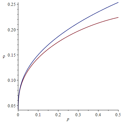
In the balanced case where all probabilities are identical, we recover the time bounds of the recently proposed ChosenPath algorithm [18], which are known to be optimal in this setting. In the very unbalanced case where some are , some are , and the expected number of items of both kinds are comparable, we match the well-known prefix filter algorithm [11], which beats ChosenPath in this setting. For skew between these extremes we get strict improvements over existing methods. (See Section 7 and Figure 1 for further discussion.)
Techniques.
Our data structure is a natural, recursive variant of ChosenPath that is able to exploit skew by varying the recursion depth over the branches of the recursion tree and by aggressively favoring choices based on the given distribution that are more likely distinguish close and far elements. We stress that ChosenPath is not able to exploit skew, and in fact has the same tight running time guarantee independent of the data distribution. Because we cut the depth of the tree earlier based on the skew of the distribution, we must tighten the previous analysis to handle sampling without replacement, while also parameterizing our performance based on skew. This leads to significant challenges.
Adversarial queries.
It may not always be reasonable to assume that a query is random and -correlated, as in Theorem 1. For this reason we analyze the setting where the query may be adversarially chosen. In Section 3 we give a data structure that adapts to the difficulty of the query, matching existing worst-case bounds for “hard” queries, while being much faster for “easy” queries. Our result uses a similarity function (defined later) to parameterize how close the query is to the nearest element of the data set.
Theorem 2.
Consider a dataset of vectors sampled from and let satisfy . Let satisfy
For any query of size satisfying for some , let satisfy
Then for any there exists a sufficiently large such that our data structure requires expected space, can be built in time, and can perform a search in time , returning with probability33 3 This probability can be increased using independent repetitions. at least .
Similarity joins.
Our results immediately apply to the problem of database similarity joins [34, 9, 30, 45, 10, 31, 2, 22].
Many similarity join algorithms work using (essentially) repeated similarity search queries; see e.g. [31, 34, 24]. This method is equally effective here. Assume that we want to find all similar pairs between sets and , and that the actual join size (i.e. the number of close pairs) is much smaller than or .44 4 If the join is large we can extend this idea via parameterizing by the join size; see e.g. the time bounds in [34, 22]. Then Theorem 2 implies that we can preprocess in time and find all pairs in time . The same idea extends to Theorem 1 as well.
1.2 Related work
Assume in the following that is large enough that the empirical correlation closely matches the true correlation.
Correlation search on the unit sphere.
After shifting vectors to have zero mean and normalizing them (which does not affect correlation), searching for a vector that is -correlated with a query vector boils down to a search problem on the unit sphere : Given find such that . In turn, this is equivalent to near neighbor search under Euclidean distance on the unit sphere, which has been studied extensively. For “balanced” data structures with space (and construction time) and query time the state-of-the-art is [5], using a non-trivial generalization of Charikar’s famous LSH for angular distances [15]. Generalizations to various time-space trade-offs are also known [17, 7].
Correlation search on sparse vectors.
For sparse binary vectors, the framework of set similarity search captures search for different notions of similarity/correlation [16]. For vectors of fixed Hamming weight there is a 1-1 correspondence between Pearson correlation and standard set similarity measures such as Jaccard similarity and Braun-Blanquet similarity. It is known that methods such as MinHash [14, 13] that specifically target sparse vectors yield better search algorithms than more general methods when the fraction of non-zero entries is bounded by a sufficiently small constant. Recently it was shown that MinHash can be improved in this setting, yielding balanced similarity search data structure with [18].
Batched search.
The first subquadratic algorithm for the light bulb problem was given by Paturi et al. [36], yielding time . Valiant [42] showed that it is possible to remove from the exponent, obtaining substantially subquadratic running time even for small values of . Karppa et al. strenthened Valiant’s result to time [26], for (where the constant 1.6 reflects current matrix multiplication algorithms). A somewhat slower, but deterministic, subquadratic algorithm was subsequently presented [27]. With the exception of [36] these methods rely on fast rectangular matrix multiplication and seem inherently only applicable to batched search problems.
Worst-Case search.
Much of previous theoretical work on set similarity search has focused on the worst case, where the point set and queries are adversarial rather than being drawn from a known distribution. The Chosen Path algorithm of Christiani and Pagh focuses on Braun-Blanquet similarity, which is the metric we use here.55 5 We show that Pearson correlated vectors are very likely to have high Braun-Blanquet similarity in Lemma 10. In particular, if the dataset contains a point where and have Braun-Blanquet similarity at least , the data structure returns a point such that and have Braun-Blanquet similarity at least . Their data structure achieves space and query time for . This result is a strict improvement over the classic MinHash algorithm [14, 13].
Lower bounds.
Cell probe data structure lower bounds achievable by current techniques are polylogarithmic in data size (assuming polylogarithmic word size). Tight bounds are only known for small query time, see e.g. [35] — for subquadratic space this leaves a large gap to the polynomial upper bounds that can be achieved by similarity search techniques. However, good conditional lower bounds based on the strong exponential time hypothesis (SETH) [23] are known. Ahle et al. [2] showed hardness of approximate maximum inner product search under SETH, but only for inner products very close to zero. Recently, Abboud, Rubinstein, and Williams [1] significantly improved this result, and in particular showed, again assuming SETH, that maximum inner product requires near-linear time even for vectors in and allowing a large approximation factor. This means that there is little hope of obtaining strong algorithms in the worst case, even for batched search problems. Of course, as the upper bounds for the light bulb problem show, the average case is easier.
Heuristics.
Above we have discussed related work with a theoretical emphasis. Many heuristics exist, especially for sparse vectors. Some of the most widely used ones are based on exact, deterministic filtering techniques, such as prefix filtering [11] which evaluates the similarity of every pair of vectors that share a in a position that has a small fraction of s. This is effective when vectors are sparse and skewed in the sense that there are many positions with a small fraction of s. We refer to Mann et al. [31] for an overview of exact, heuristic techniques.
2 Model
Our model closely follows the one in [29] — we describe it here for completeness. The elements in our set are -dimensional boolean vectors . These vectors represent a subset of items from a universe . We generally consider our elements to be boolean vectors; however, we express some of our operations using set notation for convenience (for example, represents the 1 bits in common between and ).
We are given a distribution over defined as follows: if is a vector drawn from , then independently for each . We denote by the distribution obtained by sampling vectors independently from . The probabilities are assumed to be known to the algorithm. We assume that all item-level probabilities are at most . The particular value is not important, and all of our results holds as long as there is some constant such that all item-level probabilities are bounded by .
Definition 3 (Correlation).
Let . Fix . We say that is -correlated to with respect to , written , if is a random vector drawn as follows: For each independently, with probability let , and with probability let .
If and , then the distribution of is exactly —in particular, . Furthermore, for each , the random variables and have Pearson correlation .
Our goal is to create an efficient data structure for vectors sampled from which takes advantage of possible skew in the item-level probabilities. Our performance bounds (query and preprocessing times) are expected, and depend both on and the data structure’s random choices. Following [18], we will use Braun-Blanquet similarity,
as our measure for similarity between sets. This similarity measure is closely related to Jaccard similarity, see [18] for details. We now formally define the two versions of the problem that we are considering:
Adversarial query
Given a dataset of items sampled from and a similarity threshold , preprocess into a data structure with the following capability: Given , return such that if such an exists. The data structure must succeed with probability at least over its own internal randomness. In particular, the probability that the data structure succeeds must be independent of the dataset .
Correlated query
Given a dataset of items sampled from and a correlation threshold , preprocess into a data structure with the following capability: Let and let be -correlated to with respect to . Then, given the query , the data structure must return . The data structure must succeed in doing so with probability at least over the choice of , the randomness of the dataset , and its own internal randomness.66 6 Clearly, some assumptions on the item-level probabilities of are needed for this to be possible. For all of our results, we will assume that is sufficiently large.
As usual, the part of the success probability that depends only on the data structure’s random choices may be boosted by a small number of repetitions. Thus, for adversarial queries, it suffices to build a data structure with success probability, say, , and for correlated queries, it suffices that the part of the success probability depending only on the data structure’s random choices is at least . However, the part of the success probability depending on the query and the dataset cannot be boosted by repetitions. Instead, we need to design a data structure such that under some reasonable assumptions on the item-level probabilities, we achieve the desired success probability.
We say that an event occurs with high probability if it occurs with probability for a tunable77 7 We can make arbitrarily small by adjusting other parameters. For example, in the above discussion, we can boost the probability of success from to using independent repetitions. constant .
We make use of the following weighted Chernoff bound found in e.g. [33, Ex. 4.14].
Lemma 4.
Let be independent random variables. Let , , and assume that , for . Furthermore, assume that for all , and let . Then,
3 Data Structure
The data structure follows the locality-sensitive mapping, or filtering, framework [12, 18, 17]. In this framework, each element is mapped to a set of filters . This is distinct from locality-sensitive hashing, in which would be mapped to a single hash value.
While locality-sensitive filtering is distinct from locality-sensitive hashing, preprocessing and searching follows essentially the same high-level idea.
To search for a query we iterate through each filter . For each such filter, we test all vectors such that . In other words, we iterate through each vector that has a filter in common with , and test the similarity of and . If we find a sufficiently close we return it; otherwise we return failure after exhausting all .
Thus, the goal of preprocessing is to make it easy to find elements that have a filter in common with a given query. For each filter mapped to by some element of , we store a list of all such that . These lists can be stored and accessed easily (i.e. in a hash table), and this method takes space linear in . We can preprocess quickly by calculating for all .
Thus, the goal of our data structure is to define a randomized mapping of vectors to sets of filters satisfying:
- •
If and have low similarity, then is small in expectation (guaranteeing small space and fast execution).
- •
If and have high similarity, then is non-empty with high probability (guaranteeing correctness).
Computing : the choice of paths
Our data structure is based on the Chosen Path data structure of Christiani and Pagh [18]. For our data structure, each corresponds to a path, i.e., an ordered sequence where each is the index of one of the dimensions. The construction of ensures that if , then it must hold that for all . We say that the path was chosen by if .
The data structure comes with a (deterministic) function which maps each vector , path-length and bit to a threshold . The choice of depends on the desired application and will be specified later on. In particular, is how our data structure adapts to the distribution—previous data structures essentially used a constant function for .88 8 As mentioned previously, this is not the only distinguishing technical detail. We must also sample without replacement and adjust the path length dynamically based on the probabilities of the sampled bits.
When initializing our data structure, we once and for all select hash functions, , where , each chosen independently from a family of pairwise independent hash functions. These hash functions are fixed throughout.
We now explain how to recursively compute the set of paths . Initially, let consist of the empty path. We recursively grow the paths one step at a time; in particular, contains paths of length . To demonstrate our recursive process, let be a path in . If , we stop recursing, and is a filter of . Otherwise, we independently consider each set bit of which is not already in . With probability , we concatenate to the end of ; this results in a new filter with (where denotes concatenation). This probabilistic choice is made using .
We formally define this recursive process using the following equation.
Finally, we define to be the union of all paths that stopped recursing.
We can calculate in time.
Preprocessing
During the preprocessing, we randomly select the hash functions and compute for each . Then, we use a standard dictionary data structure to construct an inverted index such that for each , we can look up .
Answering a query
For a given query we compute its chosen paths as described above (using the same hash functions as in the preprocessing). For each , we then compute for every which chose the path , i.e., for which . If an with similarity at least is found then we return . If we have exhausted all candidates without finding such an , we report that no high-similarity vector was found.
4 Correctness
We begin with a structural lemma on the number of paths two vectors and have in common. We will use this lemma to prove correctness of both of our data structures. This lemma follows the same high-level idea of the proof of correctness used in [18], but must be generalized to handle the distribution-dependent choices made by the data structures. The proof has been moved to Section 10.
Lemma 5.
Suppose that for and the following holds: For every and every , we have
| (1) |
Then, .
The following lemma is used to prove performance of our algorithms. We use an inductive argument to bound the number of paths generated by the data structure. This argument depends crucially on both the thresholds and the distribution-dependent stopping rule.
Lemma 6.
Let , and let be such that . Then . Furthermore, the expected time spend on computing is
Proof.
For , define the random variables . Let be the set of paths such that . Furthermore, let be the set of paths for which . We claim that is at most . The proof is by induction over and . Note that for every , there must exist and such that and . Thus,
Now, for every there must exist and such that for some . (The follows from taking the log of both sides of ). It follows that
We now bound the expected time for computing . To this end, note that we spend at most time in each recursive step, and that the expected number of recursive steps is at most . ∎
The next lemma shows that because we stop each branch of our recursive process once the expected number of vectors from which choses this path is constant, it follows that the expected query time is linear in .
Lemma 7.
Let , and let be such that . Furthermore, let . Then .
Proof.
From Lemma 6, we know that . Let be any path chosen by . By definition, . Thus,
5 Adversarial Queries
For the adversarial case, we set . Thus, the sampling thresholds only depend on and the number of bits already contained in the path . The remainder of the data structure follows the description in Section 3.
5.1 Correctness
We begin with a proof of correctness, giving a guarantee that if there exists an similar to a query , then and will share a filter (so will be found by our algorithm).
Fix and such that and fix . The assumption is equivalent to . Thus,
Correctness follows immediately from Lemma 5.
5.2 Performance guarantees
Query time
We bound the query time using a constant that depends only on and .
Lemma 8.
For every there exists a constant such that if and , then .
Proof.
Preprocessing time
The following lemma bounds our expected per-element processing time. The proof has been moved to Section 10.
Lemma 9.
For every there exists a constant such that if and , then for .
We multiply this by to get the expected total preprocessing time for all elements. Since our data structure takes space linear in the total size of the stored filters, we similarly obtain space.
6 Correlated Queries
We need samples from the distribution to have sufficient length such that we can guarantee that for which is not correlated with (see Lemma 10). Therefore, we assume there is a sufficiently large constant that the expected size of an element drawn from is at least . Similarly, we assume that all . We assume that .
In the correlated case, we no longer need to sample vertices uniformly at random. The query and the distribution give us further information about where and are likely to intersect. In particular, we can calculate the conditional probability
We weight our chosen path choices by this conditional probability. We then increase each sampling probability by a small constant ; this will help us ensure correctness for filters. (We derive this constant in the proof of Lemma 11. A smaller constant is likely sufficient in practice, particularly for small .) Thus, at round , we sample each bit , without replacement, with probability
With these new sampling probabilities, we again maintain paths as defined in Section 3. To answer a query , we look through all , returning any that has similarity at least .
6.1 Correctness
For a query , our data structure attempts to find the that is -correlated with by finding a similar vector among the items stored for filters in . We begin by showing that with high probability, ; meanwhile, for uncorrelated , .
Lemma 10.
Assume . With high probability, . Meanwhile, for all not correlated with , with high probability.
Proof.
To begin, note that for any , . By Chernoff bounds (Lemma 4 for example) and the union bound, with high probability for all and .
First, consider the correlated pair: . We have . Again by Chernoff, with high probability. Combining this with the above, with high probability.
Now, consider an uncorrelated pair and drawn independently from . We have . Using Chernoff bounds, with high probability. Combining with the above, with high probability. ∎
Now we show that our sampling probabilities are large enough to guarantee that the two -correlated vectors and are likely to share a path. We need to use new techniques beyond those in Section 5 (and beyond previous results) because we our proof must leverage that the close pair is chosen randomly. After all, if we ignore this aspect, we have reduced to the adversarial case—we want to improve those bounds.
We do this by showing that, with high probability, any given path during our recursive process satisfies the requirements of Lemma 5. Note that we prove correctness with probability at least for simplicity; we can obtain stronger bounds by slightly increasing .
Lemma 11.
Consider a path of length at most , and . Assume . Then, with probability at least ,
Proof.
We begin by calculating the expected value.
We have , so . Then by Lemma 4,
Assume that . Then we assign
Substituting, we obtain the lemma. ∎
Applying union bound, all paths in our recursive process satisfy Lemma 5. Thus, these two lemmas imply that we return the -correlated with high probability.
6.2 Performance Guarantees
We now compute the expected number of paths chosen by an . Since we have both and for all , this lemma implies the query time and space bounds of Theorem 1 immediately.
Lemma 12.
For every there exists a constant such that if and , then for .
Proof.
7 Performance Comparison
The bounds achieved by our data structures are given as the solution to an equation which is not in closed form. In this section, we give some examples and intuition of how much speedup we achieve.
7.1 Adversarial query
If the query is adversarial, then the query time for a query is determined by the smallest such that
We will now discuss to what extent our data structure is able to take advantage of possible skew in the item-level probabilities. In order to simplify the discussion, assume that (so that equals the expected value of when , meaning that all sets have roughly the same size). Now, for every there exists a such that if , then for every with high probability. Thus, we can solve the problem by solving the -approximate Braun-Blanquet similarity search problem using the standard Chosen Path data structure, thereby obtaining a -value which, for sufficiently large , is arbitrarily close to
If the part of the input distribution relevant for the query contains no skew, i.e., if for all , then . However, in all other cases.
To our knowledge there is no closed-form expression for the solution to the equation . Instead, we will compute in a few settings to illustrate how skew influences our query time. Suppose that consists of two types of bits: half the bits of are set with probability in a random set from , and the other half is set with probability . Furthermore, assume that .
Suppose first that the distribution has very significant skew, e.g., , . Assume that we are searching for a set in with similarity at least, say, . In this case, , whereas we obtain a -value of for sufficiently large. Prefix filtering does not give any non-trivial (worst-case) performance guarantee. This example shows that we can take advantage of the skew even when it is possible that the entire intersection between and the close point is within a part of where all bits are set with the same probability in a datapoint. A more extreme example occurs if we increase to so that a possible close point must share some of the bits for which the associated probability is . In this case, equation (7.1) is satisfied for arbitrarily close to zero. Thus, we achieve a very fast query time (in particular, our query time will be for every constant ). In order to understand why, note that no path in can contain more than two bits with associated item-level probability . Furthermore, since , our sampling threshold is low enough that we are very unlikely to create long paths consisting only of bits with associated probability . Indeed, the expected size of a path in is in this case. Solving the problem by solving the -approximate problem will yield a value of . Prefix filtering will need time to locate a possible close point if it exists.
7.2 Correlated query
When the query is -correlated with a point in our dataset , the running time is (for sufficiently large) determined by the smallest such that where .
As for the adversarial case, whenever there is significant skew in the input distribution, we can get very fast query time. Suppose for example that is such that bits are set to with probability and bits are set to with probability . If , then we find that our expected query time is for every constant . On the other hand, prefix filtering takes time.
Let us now consider examples where the input distribution is skewed but all probabilities are , meaning in particular that prefix filtering does not give any non-trivial worst-case guarantees. For example, suppose that bits are set to with probability and bits are set to with probability . We compare the performance of our data structure to that of using Chosen Path for solving the -approximate problem where is the expected similarity between the correlated points and is the expected similarity between the query and an uncorrelated point. For and and , we plot the corresponding -values in Figure 1.
8 Skew in Real Data Sets
In this section we examine how the ideas that inspired our model apply to the real-life sparse data sets used to evaluate similarity set methods by Mann et al. [31].
Skew
For each data set we computed the empirical frequencies , indexed such that frequencies decrease as grows. In Figure 2 we show the distribution of frequencies in two ways. On the left side we plot against , where is the number of vectors and is the dimension of the vectors. On the right side we show the distribution on a normalized log-log scale. As can be seen, all data sets display a significant skew. A plain Zipfian distribution would appear linear on this plot (with slope corresponding to the exponent in the distribution). Frequencies do not follow a Zipfian distribution, but are generally close to a “piecewise Zipfian” distribution. For almost all data sets, the frequencies outside of the very top can be thought of as being bounded by for some constant .
Approximate Independence
Our theoretical analysis is based on the assumption of independence between the set bits (i.e. the items) of the random vectors, and more specifically on the inequality:
| (2) |
The asymptotic analysis still applies if (2) holds only up to a constant factor. (Under some conditions we may even let this factor increase exponentially with .) To shed light on whether this assumption is realistic we considered random size-2 and size-3 subsets , respectively, and computed the expected number of vectors satisfying under the independence assumption and in the data set, respectively. The ratio of these numbers is the constant factor needed, on average over all sets , to make (2) hold.
| Data set | ||
|---|---|---|
| AOL | ||
| BMS-POS | ||
| DBLP | ||
| ENRON | ||
| FLICKR | ||
| KOSARAK | ||
| LIVEJOURNAL | ||
| NETFLIX | ||
| ORKUT | ||
| SPOTIFY |
The ratios are shown in Table 1. If the independence assumption were true, the ratios would be close to 1. As can be seen all data sets have some kind of positive correlation between dimensions meaning that there are more pairs/triples than the independence model predicts. However, for most of the data sets it seems reasonable to assume that these correlations are weak enough that (2) holds up to a constant factor independent of , at least for small constant . In those cases we expect our theoretical analysis based on independence to be indicative of actual running time.
9 Conclusion
Several open problems remain about how to handle nearest neighbor search in skewed datasets.
One natural question is how to relax the assumption that all item probabilities are known to the algorithm beforehand. It seems likely that one can estimate each to very high precision by counting the occurrences in the dataset itself, leading to the same asymptotic bounds. We note that the set similarity join algorithm in [19] avoids using or estimating , but we do not know how to analyze its performance in our setting.
The performance examples in this paper deal with distributions with two types of item: very rare and very common items. In practice, one more often encounters distributions with much more gradual skew, such as a Zipf distribution. Unfortunately, sets selected using a Zipf distribution have very small expected size, which trivializes the asymptotics. It would be interesting to find a class of distributions that accurately characterizes the skew of real data while remaining interesting for asymptotic analysis. Such a distribution would be an important use case for our algorithm.
Finally, it would be interesting to relax the independence assumption. Our experiments gave some evidence that many of the datasets we studied have only mild dependencies, but for some this was not the case (particularly the Spotify dataset). In fact, the Spotify dataset has recently been observed to be a difficult case for a variant of the Chosen Path algorithm [19], possibly due to these correlations. It seems that if the correlations are “simple” and known ahead of time, there may be strategies to deal with them when sampling paths. Such an algorithm would loosen the independence assumption in our model, and has the potential to lead to much stronger performance in practice.
10 Omitted Proofs
Proof of Lemma 5.
In order to simplify calculations, we are going to consider a conveniently chosen subset of . In order to define this subset, for and let,
We define and exactly as and , except that we replace the requirements and with the requirement . It follows from the assumption (1) that is indeed a subset of . We claim that . In order to show this, we will make use of the following second moment bound:
| (3) |
From (3), it suffices to show and for all . We will prove that this holds by induction. Recall that we start with a single empty path, and so with probability . Thus, the statement trivially holds for . Let . Define the random variable . Note that this random variable is independent of . In particular, for every possible , we have . Using this independence along with (1) yields
Recall that the hash-function was chosen from a pairwise independent family. Thus, for , we have . Then,
We have . Furthermore, (the same applies with , substituted for , respectively). Substituting,
Proof of Lemma 9.
Let and assume that for some . We want to show that if is sufficiently large, then where the expectation is over both the randomness of the data structure and the randomness of . By a Chernoff bound,
Furthermore,
When both of these events occur, we have
And therefore
Thus, according to Lemma 6, . Since is polynomial in for any , this implies that . ∎
References
- [1] A. Abboud, A. Rubinstein, and R. Williams. Distributed PCP theorems for hardness of approximation in P. In Proc. 58th Symposium on Foundations of Computer Science (FOCS), pages 25–36. IEEE, 2017.
- [2] T. D. Ahle, R. Pagh, I. Razenshteyn, and F. Silvestri. On the complexity of inner product similarity join. In Proc. 35th Symposium on Principles of Database Systems (PODS), pages 151–164. ACM, 2016.
- [3] J. Alman, T. M. Chan, and R. Williams. Polynomial representations of threshold functions and algorithmic applications. In Proc. 57th Symposium on Foundations of Computer Science (FOCS), pages 467–476. IEEE, 2016.
- [4] J. Alman and R. Williams. Probabilistic polynomials and hamming nearest neighbors. In Proc. 56th Symposium on Foundations of Computer Science (FOCS), pages 136–150. IEEE, 2015.
- [5] A. Andoni, P. Indyk, T. Laarhoven, I. Razenshteyn, and L. Schmidt. Practical and optimal LSH for angular distance. In Proc. 28th Conference on Neural Information Processing Systems (NIPS), pages 1225–1233, 2015.
- [6] A. Andoni, P. Indyk, H. L. Nguyen, and I. Razenshteyn. Beyond locality-sensitive hashing. In Proc. 25th Symposium on Discrete Algorithms (SODA), pages 1018–1028. ACM-SIAM, 2014.
- [7] A. Andoni, T. Laarhoven, I. Razenshteyn, and E. Waingarten. Optimal hashing-based time-space trade-offs for approximate near neighbors. In Proc. 28th Symposium on Discrete Algorithms (SODA), pages 47–66. ACM-SIAM, 2017.
- [8] A. Andoni and I. Razenshteyn. Optimal data-dependent hashing for approximate near neighbors. In Proc. 47th Symposium on Theory of Computing (STOC), pages 793–801. ACM, 2015.
- [9] A. Arasu, V. Ganti, and R. Kaushik. Efficient exact set-similarity joins. In Proc. 32nd International Conference on Very Large Data Bases (VLDB), pages 918–929, 2006.
- [10] N. Augsten and M. H. Böhlen. Similarity joins in relational database systems. Synthesis Lectures on Data Management, 5(5):1–124, 2013.
- [11] R. J. Bayardo, Y. Ma, and R. Srikant. Scaling up all pairs similarity search. In Proc. 16th World Wide Web Conference (WWW), pages 131–140, 2007.
- [12] A. Becker, L. Ducas, N. Gama, and T. Laarhoven. New directions in nearest neighbor searching with applications to lattice sieving. In Proc. 27th Symposium on Discrete Algorithms (SODA), pages 10–24. ACM-SIAM, 2016.
- [13] A. Z. Broder. On the resemblance and containment of documents. In Proc. Compression and Complexity of Sequences, pages 21–29. IEEE, 1997.
- [14] A. Z. Broder, S. C. Glassman, M. S. Manasse, and G. Zweig. Syntactic clustering of the web. Computer Networks and ISDN Systems, 29(8):1157–1166, 1997.
- [15] M. S. Charikar. Similarity estimation techniques from rounding algorithms. In Proc. 34th Symposium on Theory of Computing (STOC), pages 380–388. ACM, 2002.
- [16] S. Choi, S. Cha, and C. C. Tappert. A survey of binary similarity and distance measures. J. Syst. Cybern. Informatics, 8(1):43–48, 2010.
- [17] T. Christiani. A framework for similarity search with space-time tradeoffs using locality-sensitive filtering. In Proc. 28th Symposium on Discrete Algorithms (SODA), pages 31–46. ACM-SIAM, 2017.
- [18] T. Christiani and R. Pagh. Set similarity search beyond minhash. In Proc. 49th Symposium on Theory of Computing (STOC), pages 1094–1107. ACM, 2017.
- [19] T. Christiani, R. Pagh, and J. Sivertsen. Scalable and robust set similarity join. In Proc. 34th International Conference on Data Engineering (ICDE). IEEE, 2018. To appear.
- [20] S. Dasgupta and K. Sinha. Randomized partition trees for exact nearest neighbor search. In Proc. 26th Conference on Learning Theory (COLT), pages 317–337, 2013.
- [21] S. Dasgupta and K. Sinha. Randomized partition trees for nearest neighbor search. Algorithmica, 72(1):237–263, 2015.
- [22] X. Hu, Y. Tao, and K. Yi. Output-optimal parallel algorithms for similarity joins. In Proc. 36th Symposium on Principles of Database Systems (PODS), pages 79–90. ACM, 2017.
- [23] R. Impagliazzo, R. Paturi, and F. Zane. Which problems have strongly exponential complexity? J. Comput. Syst. Sci., 63(4), 2001.
- [24] Y. Jiang, D. Deng, J. Wang, G. Li, and J. Feng. Efficient parallel partition-based algorithms for similarity search and join with edit distance constraints. In Proc. Joint EDBT/ICDT Workshops, pages 341–348. ACM, 2013.
- [25] M. Kapralov. Smooth tradeoffs between insert and query complexity in nearest neighbor search. In Proc. 34th Symposium on Principles of Database Systems (PODS), pages 329–342. ACM, 2015.
- [26] M. Karppa, P. Kaski, and J. Kohonen. A faster subquadratic algorithm for finding outlier correlations. In Proc. 27th Symposium on Discrete Algorithms (SODA). ACM-SIAM, 2016.
- [27] M. Karppa, P. Kaski, J. Kohonen, and P. Ó. Catháin. Explicit correlation amplifiers for finding outlier correlations in deterministic subquadratic time. In Proc. 24th European Symposium on Algorithms (ESA), pages 52:1–52:17, 2016.
- [28] O. Keivani, K. Sinha, and P. Ram. Improved maximum inner product search with better theoretical guarantees. In Proc. International Joint Conference on Neural Networks (IJCNN), pages 2927–2934, 2017.
- [29] A. Kirsch, M. Mitzenmacher, A. Pietracaprina, G. Pucci, E. Upfal, and F. Vandin. An efficient rigorous approach for identifying statistically significant frequent itemsets. Journal of the ACM (JACM), 59(3):12, 2012.
- [30] G. Li, D. Deng, J. Wang, and J. Feng. Pass-join: A partition-based method for similarity joins. Proc. 37th International Conference on Very Large Data Bases, 5(3):253–264, 2011.
- [31] W. Mann, N. Augsten, and P. Bouros. An empirical evaluation of set similarity join techniques. Proc. 42nd International Conference on Very Large Data Bases, 9(9):636–647, 2016.
- [32] A. May and I. Ozerov. On computing nearest neighbors with applications to decoding of binary linear codes. In Proc. 34th International Conference on the Theory and Applications of Cryptographic Techniques (EUROCRYPT), pages 203–228, 2015.
- [33] M. Mitzenmacher and E. Upfal. Probability and computing - randomized algorithms and probabilistic analysis. Cambridge University Press, 2005.
- [34] R. Pagh, N. Pham, F. Silvestri, and M. Stöckel. I/O-efficient similarity join. In Proc. 23rd European Symposium on Algorithms (ESA), pages 941–952, 2015.
- [35] R. Panigrahy, K. Talwar, and U. Wieder. Lower bounds on near neighbor search via metric expansion. In Proc. 51st Symposium on Foundations of Computer Science (FOCS), pages 805–814. IEEE, 2010.
- [36] R. Paturi, S. Rajasekaran, and J. H. Reif. The light bulb problem. In Proc. 2nd Workshop on Computational Learning Theory (COLT), pages 261–268, 1989.
- [37] P. Ram and A. G. Gray. Maximum inner-product search using cone trees. In Proc. 18th International Conference on Knowledge Discovery and Data Mining (KDD), pages 931–939. ACM, 2012.
- [38] A. Shrivastava and P. Li. Asymmetric LSH (ALSH) for sublinear time maximum inner product search (MIPS). In Proc. 27th Conference on Neural Information Processing Systems (NIPS), pages 2321–2329, 2014.
- [39] A. Shrivastava and P. Li. Asymmetric minwise hashing for indexing binary inner products and set containment. In Proc. 24th International Conference on World Wide Web (WWW), pages 981–991, 2015.
- [40] A. Shrivastava and P. Li. Improved asymmetric locality sensitive hashing (ALSH) for maximum inner product search (MIPS). In Proc. 31st Conference on Uncertainty in Artificial Intelligence (UAI), pages 812–821, 2015.
- [41] C. Teflioudi, R. Gemulla, and O. Mykytiuk. LEMP: Fast retrieval of large entries in a matrix product. In Proc. 41st International Conference on Management of Data (SIGMOD), pages 107–122. ACM, 2015.
- [42] G. Valiant. Finding correlations in subquadratic time, with applications to learning parities and the closest pair problem. J. ACM, 62(2):13:1–13:45, 2015.
- [43] L. G. Valiant. Functionality in neural nets. In Proc. 7th National Conference on Artificial Intelligence (AAAI), pages 629–634, 1988.
- [44] J. Wang, G. Li, and J. Feng. Can we beat the prefix filtering?: an adaptive framework for similarity join and search. In Proc. 38th International Conference on Management of Data (SIGMOD), pages 85–96. ACM, 2012.
- [45] C. Xiao, W. Wang, X. Lin, and J. X. Yu. Efficient similarity joins for near duplicate detection. In Proc. International Conference on World Wide Web (WWW), pages 131–140, 2008.
- [46] H. Zhang and Q. Zhang. Embedjoin: Efficient edit similarity joins via embeddings. In Proceedings of International Conference on Knowledge Discovery and Data Mining (KDD), pages 585–594. ACM, 2017.