跳到论文正文
W Papers独立论文阅读器 arXiv:1804.02829 论文正文 计算阅读时间 · 0%
引用这篇论文根据当前论文元数据生成,正式投稿前建议核对。


License: arXiv.org perpetual non-exclusive license
arXiv:1804.02829v1 [math.OC] 09 Apr 2018

Optimal Covariance Control for Stochastic Systems
Under Chance Constraints

Kazuhide Okamoto ††thanks: K. Okamoto is a Ph.D. Candidate at the School of Aerospace Engineering, Georgia Institute of Technology, Atlanta, GA 30332-0150, USA. Email: kazuhide@gatech.edu    Maxim Goldshtein ††thanks: M. Goldshtein is a PhD Student at the School of Aerospace Engineering, Georgia Institute of Technology, Atlanta, GA 30332-0150, USA. Email:maxg@gatech.edu    Panagiotis Tsiotras ††thanks: P. Tsiotras is a Professor at the School of Aerospace Engineering and the Institute for Robotics & Intelligent Machines, Georgia Institute of Technology, Atlanta, GA 30332-0150, USA. Email: tsiotras@gatech.edu
Abstract

This work addresses the optimal covariance control problem for stochastic discrete-time linear time-varying systems subject to chance constraints. Covariance steering is a stochastic control problem to steer the system state Gaussian distribution to another Gaussian distribution while minimizing a cost function. To the best of our knowledge, covariance steering problems have never been discussed with probabilistic chance constraints although it is a natural extension. In this work, first we show that, unlike the case with no chance constraints, the covariance steering with chance constraints problem cannot decouple the mean and covariance steering sub-problems. Then we propose an approach to solve the covariance steering with chance constraints problem by converting it to a semidefinite programming problem. The proposed algorithm is verified using two simple numerical simulations.

1 Introduction

In this work we address a problem of finite-horizon stochastic optimal control for a discrete-time linear time-varying stochastic system with a fully-observable state, a given Gaussian distribution of the initial state, and a state and input-independent white-noise Gaussian diffusion with given statistics. The control task is to steer the system state to the target Gaussian distribution, while minimizing a state and control expectation-dependent cost. In addition to the boundary condition, in the aim of adding robustness to the controller under stochastic uncertainty, we consider chance constraints, which restricts the probability of violating the state constraints to be less than a pre-specified threshold.

Since the Gaussian distribution can be fully defined by its first two moments, this problem can be described as a finite-time optimal mean and covariance steering of a stochastic time-varying discrete linear system, with a boundary conditions in form of given initial and final mean and covariance, and with constraints on the trajectory in form of probability function.

This chance-constrained optimal covariance control problem is relevant to a wide range of control and planning task, such as decentralized control of swarm robots [1], closed-loop cooling [2], and others, in which the state is more naturally described by it’s distribution, rather than a fixed set of values. In addition, this approach is readily-applicable to a stochastic MPC framework [3].

Covariance steering problem

The problem of controlling the state covariance of a linear system goes back to the late 80s. The so-called covariance steering (or “Covariance Assignment”) problem was first introduced by Hotz and Skelton [4], where they computed the state feedback gains of a linear time-invariant system, such that the state covariance converges to a pre-specified value. Since then, many works have been devoted to this problem of infinite-horizon covariance assignment, both for continuous and discrete time systems [5, 6, 7, 8, 9]. Recently, the finite-horizon covariance control problem has been investigated by a number of researchers [10, 11, 12, 13, 14], relating to the problems of Shrödinger bridges [15] and the Optimal Mass Transfer [16]. Others, including our previous work, showed that the finite covariance control problem solution can be seen as a LQG with a particular weights [17, 18], which can be also formulated (and solved) as a LMI problem [19, 20, 21].

Chance-constrained control

A chance-constrained optimization has been extensively studied since 50’s, with purpose of system design with guaranteed performance under uncertainty [22]. A stochastic model-predictive control design with a chance-constraints has been solved using various techniques (see [23] for an extensive review).

Main contribution

The current paper contributes to this line of work by adding chance state constraints to the underlying stochastic optimal covariance steering problem. The covariance control problem is reformulated as an LMI, with a decision variable that is quadratic in the cost function. The chance constrains are presented as a deterministic constraint on the mean and the covariance, and added to the LMI formulation, allowing an efficient solution with any generic LMI solvers.

To the best of the authors’ knowledge, this work is the first that solves the covariance-steering problem with chance constraints.

Paper structure

The remainder of this paper is organized as follows. Section 2 formulates the problem we wish to address in this paper. We consider a time-varying stochastic linear system and a general L2L_{2}-norm objective function. Before introducing the proposed approach to deal with the chance constraints, in Section 3, we describe the case without chance constraints, in which case the mean and covariance steering part can be nicely decoupled into two independent subproblems, namely, one for the mean and one for the second moment of the state. In Section 4 we provide the solution to the covariance steering problem with chance constraints and we show how the solution of the problem can be cast as a convex optimization problem. In Section 5 we validate the effectiveness of the proposed approach via numerical simulations. Finally, Section 6 briefly summarizes the contribution of this work and proposes some possible future research directions.

2 Problem Statement

In this section we formulate the finite-horizon optimal covariance control problem for a stochastic, linear, time-varying system in discrete-time subject to chance constraints. We then reformulate the problem using concatenated state, input, and noise vectors and transition matrices.

2.1 Problem Formulation

We consider the following discrete-time stochastic linear system (possibly time-varying) with additive uncertainty, described by the equations

xk+1=Ak​xk+Bk​uk+Dk​wk,x_{k+1}=A_{k}x_{k}+B_{k}u_{k}+D_{k}w_{k}, (1)

where k=0,1,…,N−1k=0,1,\ldots,N-1 is the time step, x∈ℝnxx\in\mathbb{R}^{n_{x}} is the state, u∈ℝnuu\in\mathbb{R}^{n_{u}} is the control input, and w∈ℝnww\in\mathbb{R}^{n_{w}} is a zero-mean white Gaussian noise with unit covariance, that is,

𝔼⁡[wk]=0,𝔼⁡[wk1​wk2⊤]={Inw,if ​k1=k2,0,otherwise.\mathbb{E}\left[w_{k}\right]=0,\qquad\qquad\mathbb{E}\left[w_{k_{1}}{w_{k_{2}}^{\top}}\right]=\begin{cases}I_{n_{w}},&\mbox{if }k_{1}=k_{2},\\ 0,&\mbox{otherwise.}\end{cases} (2)

We also assume that

𝔼⁡[xk1​wk2⊤]=0,0≤k1≤k2≤N.\mathbb{E}\left[x_{k_{1}}w_{k_{2}}^{\top}\right]=0,\qquad 0\leq k_{1}\leq k_{2}\leq N. (3)

The initial state x0x_{0} is a random vector that is drawn from the multi-variate normal distribution

x0∼𝒩⁡(μ0,Σ0),x_{0}\sim\mathcal{N}(\mu_{0},\Sigma_{0}), (4)

where μ0∈ℝnx\mu_{0}\in\mathbb{R}^{n_{x}} is the initial state mean and Σ0∈ℝnx×nx\Sigma_{0}\in\mathbb{R}^{n_{x}\times n_{x}} is the initial state covariance. We assume that Σ0⪰0\Sigma_{0}\succeq 0. Our objective is to steer the trajectories of the system (1) from this initial distribution to the terminal Gaussian distribution

xN∼𝒩⁡(μN,ΣN),x_{N}\sim\mathcal{N}(\mu_{N},\Sigma_{N}), (5)

where μN∈ℝnx\mu_{N}\in\mathbb{R}^{n_{x}} and ΣN∈ℝnx×nx\Sigma_{N}\in\mathbb{R}^{n_{x}\times n_{x}} with ΣN≻0\Sigma_{N}\succ 0, at a given time NN, while minimizing the cost function

J⁡(x0,…,xN−1,u0,…,uN−1)=𝔼⁡[∑k=0N−1xk⊤​Qk​xk+uk⊤​Rk​uk],J(x_{0},\ldots,x_{N-1},u_{0},\ldots,u_{N-1})=\mathbb{E}\left[\sum_{k=0}^{N-1}x_{k}^{\top}Q_{k}x_{k}+u_{k}^{\top}R_{k}u_{k}\right], (6)

where Qk⪰0Q_{k}\succeq 0 and Rk≻0R_{k}\succ 0 for all k=0,1,…,N−1k=0,1,\ldots,N-1.

Note that (6) does not include a terminal cost owing to the terminal constraint (5). The objective is to compute the optimal control input, which ensures that the probability of the state violation at any given time is below a pre-specified threshold, say,

Pr(xk∉χ)≤Pfail,k=0,…,N,\texttt{Pr}(x_{k}\notin\chi)\leq P_{\rm{fail}},\qquad k=0,\ldots,N, (7)

where Pr​()\texttt{Pr}() denotes the probability of an event, χ⊂ℝnx\chi\subset\mathbb{R}^{n_{x}} is the state constraint set, and Pfail∈[0,1]P_{\rm{fail}}\in[0,1] is the threshold for the probability of failure. Note that μ0\mu_{0}, μN\mu_{N}, Σ0\Sigma_{0}, and ΣN\Sigma_{N} need to be designed to satisfy this chance constraint. Optimization problems with these types of constraints are known as the chance-constrained optimization problems [24]. In this work, we assume for simplicity that χ\chi is convex, but chance-constraints with non-convex constraints are also possible (see, for instance, [25])

It is assumed that the system (1) is controllable, that is xNx_{N} is reachable for any xN∈ℝnxx_{N}\in\mathbb{R}^{n_{x}}, provided that wk=0w_{k}=0 for k∈[0,N−1]k\in[0,N-1]. This implies that given any xN∈ℝnxx_{N}\in\mathbb{R}^{n_{x}} and x0∈ℝnxx_{0}\in\mathbb{R}^{n_{x}}, there exists a sequence of control inputs {uk}k=0N−1\{u_{k}\}_{k=0}^{N-1} that steers x0x_{0} to xNx_{N}.

2.2 Preliminaries

We provide an alternative description of the system dynamics in (1) that will be instrumental for solving the problem. The discussion below is borrowed from [18].

At each time step kk, we explicitly compute the system state xkx_{k} as follows. Let Ak1,k0A_{k_{1},k_{0}}, Bk1,k0B_{k_{1},k_{0}}, and Dk1,k0D_{k_{1},k_{0}}, where k1>k0k_{1}>k_{0}, denote the transition matrices of the state, input, and the noise term from step k0k_{0} to step k1+1k_{1}+1, respectively, as follows

Ak1,k0=Ak1Ak1−1⋯Ak0,\displaystyle A_{k_{1},k_{0}}=A_{k_{1}}A_{k_{1}-1}\cdots A_{k_{0}}, (8a)
Bk1,k0=Ak1,k0+1​Bk0,\displaystyle B_{k_{1},k_{0}}=A_{k_{1},k_{0}+1}B_{k_{0}}, (8b)
Dk1,k0=Ak1,k0+1​Dk0.\displaystyle D_{k_{1},k_{0}}=A_{k_{1},k_{0}+1}D_{k_{0}}. (8c)

We define the augmented vectors Uk∈ℝ(k+1)​nuU_{k}\in\mathbb{R}^{(k+1)n_{u}} and Wk∈ℝ(k+1)​nwW_{k}\in\mathbb{R}^{(k+1)n_{w}} as

Uk=[u0u1uk],Wk=[w0w1wk].U_{k}=\begin{bmatrix}u_{0}\\ u_{1}\\ \vdots\\ u_{k}\end{bmatrix},\qquad W_{k}=\begin{bmatrix}w_{0}\\ w_{1}\\ \vdots\\ w_{k}\end{bmatrix}. (9)

Then xkx_{k} can be equivalently computed from

xk=A¯k​x0+B¯k​Uk+D¯k​Wk,x_{k}=\bar{A}_{k}x_{0}+\bar{B}_{k}U_{k}+\bar{D}_{k}W_{k}, (10)

where

A¯k=Ak−1,0,\displaystyle\bar{A}_{k}=A_{k-1,0}, (11a)
B¯k=[Bk−1,0Bk−1,1⋯Bk−1],\displaystyle\bar{B}_{k}=\begin{bmatrix}B_{k-1,0}&B_{k-1,1}&\cdots&B_{k-1}\end{bmatrix}, (11b)
D¯k=[Dk−1,0Dk−1,1⋯Dk−1].\displaystyle\bar{D}_{k}=\begin{bmatrix}D_{k-1,0}&D_{k-1,1}&\cdots&D_{k-1}\end{bmatrix}. (11c)

Furthermore, we introduce the augmented state vector X∈ℝ(k+1)​nxX\in\mathbb{R}^{(k+1)n_{x}} as follows

Xk=[x0x1xk].X_{k}=\begin{bmatrix}x_{0}\\ x_{1}\\ \vdots\\ x_{k}\end{bmatrix}. (12)

It follows that the system dynamics (1) take the equivalent form

X=𝒜​x0+ℬ​U+𝒟​W,X=\mathcal{A}x_{0}+\mathcal{B}U+\mathcal{D}W, (13)

where X=XN∈ℝ(N+1)​nxX=X_{N}\in\mathbb{R}^{(N+1)n_{x}}, U=UN−1∈ℝN​nuU=U_{N-1}\in\mathbb{R}^{Nn_{u}}, and W=WN−1∈ℝN​nwW=W_{N-1}\in\mathbb{R}^{Nn_{w}}, and the matrices 𝒜∈ℝ(N+1)​nx×nx\mathcal{A}\in\mathbb{R}^{(N+1)n_{x}\times n_{x}}, ℬ∈ℝ(N+1)​nx×N​nu\mathcal{B}\in\mathbb{R}^{(N+1)n_{x}\times Nn_{u}}, and 𝒟∈ℝ(N+1)​nx×N​nw\mathcal{D}\in\mathbb{R}^{(N+1)n_{x}\times Nn_{w}} are defined as

𝒜=[IA¯1A¯2A¯N],ℬ=[00⋯0B00⋯0B1,0B1⋯0BN−1,0BN−1,1⋯BN−1],\mathcal{A}=\begin{bmatrix}I\\ \bar{A}_{1}\\ \bar{A}_{2}\\ \vdots\\ \bar{A}_{N}\end{bmatrix},\qquad\qquad\mathcal{B}=\begin{bmatrix}0&0&\cdots&0\\ B_{0}&0&\cdots&0\\ B_{1,0}&B_{1}&\cdots&0\\ \vdots&\vdots&\vdots&\vdots\\ B_{N-1,0}&B_{N-1,1}&\cdots&B_{N-1}\end{bmatrix}, (14a)
and
𝒟=[00⋯0D00⋯0D1,0D1⋯0DN−1,0DN−1,1⋯DN−1].\mathcal{D}=\begin{bmatrix}0&0&\cdots&0\\ D_{0}&0&\cdots&0\\ D_{1,0}&D_{1}&\cdots&0\\ \vdots&\vdots&\vdots&\vdots\\ D_{N-1,0}&D_{N-1,1}&\cdots&D_{N-1}\end{bmatrix}. (14b)

Note that

𝔼⁡[x0​x0⊤]\displaystyle\mathbb{E}[x_{0}x_{0}^{\top}] =Σ0+μ0​μ0⊤,\displaystyle=\Sigma_{0}+\mu_{0}\mu_{0}^{\top}, (15a)
𝔼⁡[x0​W⊤]\displaystyle\mathbb{E}[x_{0}W^{\top}] =0,\displaystyle=0, (15b)
𝔼⁡[W​W⊤]\displaystyle\mathbb{E}[WW^{\top}] =IN​nw.\displaystyle=I_{Nn_{w}}. (15c)

Using the previous expressions for XX and UU, we may rewrite the objective function in (6) as follows

J⁡(X,U)=𝔼⁡[X⊤​Q¯​X+U⊤​R¯​U],J(X,U)=\mathbb{E}\left[X^{\top}\bar{Q}X+U^{\top}\bar{R}U\right], (16)

where Q¯=blkdiag​(Q0,Q1,…,QN−1,0)∈ℝ(N+1)​nx×(N+1)​nx\bar{Q}=\texttt{blkdiag}(Q_{0},Q_{1},\ldots,Q_{N-1},0)\in\mathbb{R}^{(N+1)n_{x}\times(N+1)n_{x}} and R¯=blkdiag​(R0,R1,…,RN−1)∈ℝN​nu×N​nu\bar{R}=\texttt{blkdiag}(R_{0},R_{1},\ldots,R_{N-1})\in\mathbb{R}^{Nn_{u}\times Nn_{u}}. Note that, since Qk⪰0Q_{k}\succeq 0 and Rk≻0R_{k}\succ 0 for all k=0,1,…,N−1k=0,1,\ldots,N-1, it follows that Q¯⪰0\bar{Q}\succeq 0 and R¯≻0\bar{R}\succ 0.

The boundary conditions (4) and (5) also take the form

μ0\displaystyle\mu_{0} =E0​𝔼​[X],\displaystyle=E_{0}\mathbb{E}[X], (17a)
Σ0\displaystyle\Sigma_{0} =E0​(𝔼⁡[X​X⊤]−𝔼⁡[X]​𝔼​[X]⊤)​E0⊤,\displaystyle=E_{0}\left(\mathbb{E}[XX^{\top}]-\mathbb{E}[X]\mathbb{E}[X]^{\top}\right)E_{0}^{\top}, (17b)

and

μN\displaystyle\mu_{N} =EN​𝔼​[X],\displaystyle=E_{N}\mathbb{E}[X], (18a)
ΣN\displaystyle\Sigma_{N} =EN​(𝔼⁡[X​X⊤]−𝔼⁡[X]​𝔼​[X]⊤)​EN⊤,\displaystyle=E_{N}\left(\mathbb{E}[XX^{\top}]-\mathbb{E}[X]\mathbb{E}[X]^{\top}\right)E_{N}^{\top}, (18b)

where E0≜[Inx,0,…,0]∈ℝnx×(N+1)​nxE_{0}\triangleq\left[I_{n_{x}},0,\ldots,0\right]\in\mathbb{R}^{n_{x}\times(N+1)n_{x}} and EN≜[0,…,0,Inx]∈ℝnx×(N+1)​nxE_{N}\triangleq\left[0,\ldots,0,I_{n_{x}}\right]\in\mathbb{R}^{n_{x}\times(N+1)n_{x}}, respectively.

Finally, the chance constraints (7) can be rewritten as

Pr​(X∉𝒳)≤Pfail,\texttt{Pr}(X\notin\mathcal{X})\leq P_{\rm{fail}}, (19)

where 𝒳⊂ℝ(N+1)​nx\mathcal{X}\subset\mathbb{R}^{(N+1)n_{x}} is a convex set.

The objective of this paper is to solve the following problem.

Problem 1.

Given the system (13), find the control sequence U∗U^{\ast} that minimizes the cost function Eq. (16) subject to the initial state constraints (17), the terminal state constraints (18), and the chance constraint (19).

In Section 4 we show how to solve Problem 1 by converting it to a convex programming problem. Before doing that, we first investigate the case without chance constraints. The investigation of this case will clarify the difference of our work from prior research works on covariance steering, where the mean of the initial and terminal Gaussian distribution constraints are assumed to be zero.

3 No Chance Constraint Case

Before discussing the general case with chance constraints, in this section we introduce the case without chance constraints and show that, similarly to the work by Goldshtein and Tsiotras [18], where the authors considered the case with minimal control effort, it is possible to separately solve the mean and the covariance steering optimization problems, even with the more general ℓ2\ell_{2}-norm objective function of equation (6).

3.1 Separation of Mean and Covariance Problems

In [18] the authors showed that it is possible to separate the mean and the covariance evolutions of the system. Along with a similar separation of the cost, this observation allowed to independently design a mean-steering and a covariance-steering controller independently from one another. In this section we show that a similar result holds for the cost (6). While the objective function in [18] had only a control penalty term

J⁡(U)=𝔼⁡[∑k=0N−1uk⊤​uk],J(U)=\mathbb{E}[\sum_{k=0}^{N-1}u_{k}^{\top}u_{k}], (20)

in this paper we work with the more general cost (6). First, it follows immediately from Eq. (10) that

μk≜𝔼⁡[xk]=A¯k​μ0+B¯k​U¯k,\mu_{k}\triangleq\mathbb{E}[x_{k}]=\bar{A}_{k}\mu_{0}+\bar{B}_{k}\bar{U}_{k}, (21)

where U¯k=𝔼⁡[Uk]\bar{U}_{k}=\mathbb{E}[U_{k}]. Furthermore, by defining

U~k≜Uk−U¯k,x~k≜xk−μk,\tilde{U}_{k}\triangleq U_{k}-\bar{U}_{k},\qquad\tilde{x}_{k}\triangleq x_{k}-\mu_{k}, (22)

and using (10), the following equation holds for x~k\tilde{x}_{k}

x~k=A¯k​x~0+B¯k​U~k+D¯k​Wk.\tilde{x}_{k}=\bar{A}_{k}\tilde{x}_{0}+\bar{B}_{k}\tilde{U}_{k}+\bar{D}_{k}W_{k}. (23)

Furthermore,

Σk\displaystyle\Sigma_{k} ≜𝔼⁡[x~k​x~k⊤],\displaystyle\triangleq\mathbb{E}[\tilde{x}_{k}\tilde{x}_{k}^{\top}], (24a)
=𝔼⁡[(A¯k​x~0+B¯k​U~k+D¯k​Wk)​(A¯k​x~0+B¯k​U~k+D¯k​Wk)⊤],\displaystyle=\mathbb{E}\left[\big(\bar{A}_{k}\tilde{x}_{0}+\bar{B}_{k}\tilde{U}_{k}+\bar{D}_{k}W_{k}\right)\left(\bar{A}_{k}\tilde{x}_{0}+\bar{B}_{k}\tilde{U}_{k}+\bar{D}_{k}W_{k}\big)^{\top}\right], (24b)
=A¯k​𝔼​[x~0​x~0⊤]​A¯k⊤+A¯k​𝔼​[x~0​U~k⊤]​B¯k⊤+B¯k​𝔼​[U~k​x~0⊤]​A¯k⊤+B¯k​𝔼​[U~k​U~k⊤]​B¯k⊤\displaystyle=\bar{A}_{k}\mathbb{E}[\tilde{x}_{0}\tilde{x}_{0}^{\top}]\bar{A}_{k}^{\top}+\bar{A}_{k}\mathbb{E}[\tilde{x}_{0}\tilde{U}_{k}^{\top}]\bar{B}_{k}^{\top}+\bar{B}_{k}\mathbb{E}[\tilde{U}_{k}\tilde{x}_{0}^{\top}]\bar{A}_{k}^{\top}+\bar{B}_{k}\mathbb{E}[\tilde{U}_{k}\tilde{U}_{k}^{\top}]\bar{B}_{k}^{\top}
+D¯k​𝔼​[Wk​Wk⊤]​D¯k⊤+D¯k−1​𝔼​[Wk−1​U~k⊤]​B¯k⊤+B¯k​𝔼​[U~k​Wk−1⊤]​D¯k−1⊤.\displaystyle\hskip 56.9055pt+\bar{D}_{k}\mathbb{E}[{W}_{k}{W}_{k}^{\top}]\bar{D}_{k}^{\top}+\bar{D}_{k-1}\mathbb{E}[{W}_{k-1}\tilde{U}_{k}^{\top}]\bar{B}_{k}^{\top}+\bar{B}_{k}\mathbb{E}[\tilde{U}_{k}{W}_{k-1}^{\top}]\bar{D}_{k-1}^{\top}. (24c)

Note that the evolution of the mean μk\mu_{k} from (21) depends only on U¯k\bar{U}_{k}, whereas the evolution of x~k\tilde{x}_{k} and Σk\Sigma_{k} depend solely on U~k\tilde{U}_{k} and WkW_{k}. It follows from Eq. (13) and (21) that

X¯≜𝔼⁡[X]=𝒜​μ0+ℬ​U¯,\bar{X}\triangleq\mathbb{E}[X]=\mathcal{A}\mu_{0}+\mathcal{B}\bar{U}, (25)

and from (23) that

X~≜X−𝔼⁡[X]=𝒜​x~0+ℬ​U~+𝒟​W.\tilde{X}\triangleq X-\mathbb{E}[X]=\mathcal{A}\tilde{x}_{0}+\mathcal{B}\tilde{U}+\mathcal{D}W. (26)

The objective function (16) can also be rewritten as follows

J⁡(X,U)\displaystyle J(X,U) =𝔼⁡[X⊤​Q¯​X+U⊤​R¯​U]\displaystyle=\mathbb{E}\left[X^{\top}\!\bar{Q}X+U^{\top}\!\bar{R}U\right] (27a)
=𝚝𝚛⁡(Q¯​𝔼​[X~​X~⊤])+X¯⊤​Q¯​X¯+𝚝𝚛⁡(R¯​𝔼​[U~​U~⊤])+U¯⊤​R¯​U¯,\displaystyle=\mathtt{tr}\big(\bar{Q}\,\mathbb{E}[\tilde{X}\tilde{X}^{\top}]\big)+\bar{X}^{\top}\!\bar{Q}\bar{X}+\mathtt{tr}\big(\bar{R}\mathbb{E}[\tilde{U}\tilde{U}^{\top}]\big)+\bar{U}^{\top}\!\bar{R}\bar{U}, (27b)
=Jμ​(X¯,U¯)+JΣ​(X~,U~),\displaystyle=J_{\mu}(\bar{X},\bar{U})+J_{\Sigma}(\tilde{X},\tilde{U}), (27c)

where

Jμ​(X¯,U¯)=X¯⊤​Q¯​X¯+U¯⊤​R¯​U¯,J_{\mu}(\bar{X},\bar{U})=\bar{X}^{\top}\bar{Q}\bar{X}+\bar{U}^{\top}\bar{R}\bar{U}, (28)

and

JΣ​(X~,U~)=𝚝𝚛⁡(Q¯​𝔼​[X~​X~⊤])+𝚝𝚛⁡(R¯​𝔼​[U~​U~⊤]),J_{\Sigma}(\tilde{X},\tilde{U})=\mathtt{tr}\big(\bar{Q}\mathbb{E}[\tilde{X}\tilde{X}^{\top}]\big)+\mathtt{tr}\big(\bar{R}\mathbb{E}[\tilde{U}\tilde{U}^{\top}]\big), (29)

and where tr​()\texttt{tr}() denotes the trace of a matrix. It follows that the original optimization problem in terms of (X,U)(X,U) is equivalent to two separate optimization problems in terms of (X¯,U¯)(\bar{X},\bar{U}) and (X~,U~)(\tilde{X},\tilde{U}) with optimization costs (28) and (29), respectively.

We have therefore shown the following result.

Proposition 1.

Let the system (13), the initial and terminal state constraints (4) and (5), and the objective function (6). The control sequence U∗U^{*} that solves this optimization problem is given by U∗=U¯∗+U~∗U^{*}=\bar{U}^{*}+\tilde{U}^{*}, where U¯∗\bar{U}^{*} solves the optimization problem

Mean Steering{min(X¯,U¯)⁡Jμ​(X¯,U¯)=X¯⊤Q¯​X¯+U¯⊤​R¯​U¯subject​toX¯=𝒜​μ0+ℬ​U¯,E0​X¯=μ0,EN​X¯=μN,\text{Mean Steering}\left\{\begin{aligned} \min_{(\bar{X},\bar{U})}J_{\mu}(\bar{X},\bar{U})=\bar{X}^{\top}&\bar{Q}\bar{X}+\bar{U}^{\top}\bar{R}\bar{U}\\ \mathrm{subject\penalty\ to}\penalty\ \penalty\ \bar{X}=\mathcal{A}\mu_{0}&+\mathcal{B}\bar{U},\\ E_{0}\bar{X}=\mu_{0},\penalty\ \penalty\ &E_{N}\bar{X}=\mu_{N},\end{aligned}\right. (30)

and U~∗\tilde{U}^{*} solves the optimization problem

Covariance Steering{min(X~,U~)JΣ(X~,U~)=𝚝𝚛(Q¯𝔼[X~X~⊤])+𝚝𝚛(R¯𝔼[U~U~⊤]),subject​toX~≜X−𝔼⁡[X]=𝒜​x~0+ℬ​U~+𝒟​WE0​X~​X~⊤​E0⊤=Σ0,EN​X~​X~⊤​EN⊤=ΣN.\text{Covariance Steering}\left\{\begin{aligned} \min_{(\tilde{X},\tilde{U})}J_{\Sigma}(\tilde{X},\tilde{U})=\mathtt{tr}\big(\bar{Q}\mathbb{E}[&\tilde{X}\tilde{X}^{\top}]\big)+\mathtt{tr}\big(\bar{R}\mathbb{E}[\tilde{U}\tilde{U}^{\top}]\big),\\ \mathrm{subject\penalty\ to}\penalty\ \penalty\ \tilde{X}\triangleq X-\mathbb{E}[X]&=\mathcal{A}\tilde{x}_{0}+\mathcal{B}\tilde{U}+\mathcal{D}W\\ E_{0}\tilde{X}\tilde{X}^{\top}E_{0}^{\top}=\Sigma_{0},&\penalty\ \penalty\ E_{N}\tilde{X}\tilde{X}^{\top}E_{N}^{\top}=\Sigma_{N}.\end{aligned}\right. (31)

The rest of this section introduces the methods to solve these two subproblems.

3.2 Optimal Mean Steering

The solution to the optimal mean steering subproblem is summarized in the following proposition.

Proposition 2.

The optimal control sequence that solves the optimization problem (30) is given by

U¯∗=ℛ−1​(ℬ⊤​Q¯​𝒜​μ0+B¯N⊤​(B¯N​ℛ−1​B¯N⊤)−1​(μN−A¯N​μ0−B¯N​ℛ−1​ℬ⊤​Q¯​𝒜​μ0)),\bar{U}^{\ast}=\mathcal{R}^{-1}\left(\mathcal{B}^{\top}\bar{Q}\mathcal{A}\mu_{0}+\bar{B}_{N}^{\top}(\bar{B}_{N}\mathcal{R}^{-1}\bar{B}_{N}^{\top})^{-1}\left(\mu_{N}-\bar{A}_{N}\mu_{0}-\bar{B}_{N}\mathcal{R}^{-1}\mathcal{B}^{\top}\bar{Q}\mathcal{A}\mu_{0}\right)\right), (32)

where ℛ=(ℬ⊤​Q¯​ℬ+R¯)\mathcal{R}=(\mathcal{B}^{\top}\bar{Q}\mathcal{B}+\bar{R}).

Proof.

Since the terminal constraint is μN=EN​X¯=A¯N​μ0+B¯N​U¯\mu_{N}=E_{N}\bar{X}=\bar{A}_{N}\mu_{0}+\bar{B}_{N}\bar{U} we can write the Lagrangian as

ℒ⁡(U¯,λ)\displaystyle\mathcal{L}(\bar{U},\lambda) =X¯⊤​Q¯​X¯+U¯⊤​R¯​U¯+λ⊤​(μN−A¯N​μ0−B¯N​U¯)\displaystyle=\bar{X}^{\top}\bar{Q}\bar{X}+\bar{U}^{\top}\bar{R}\bar{U}+\lambda^{\top}(\mu_{N}-\bar{A}_{N}\mu_{0}-\bar{B}_{N}\bar{U}) (33)
=(𝒜​μ0+ℬ​U¯)⊤​Q¯​(𝒜​μ0+ℬ​U¯)+U¯⊤​R¯​U¯+λ⊤​(μN−A¯N​μ0−B¯N​U¯),\displaystyle=(\mathcal{A}\mu_{0}+\mathcal{B}\bar{U})^{\top}\bar{Q}(\mathcal{A}\mu_{0}+\mathcal{B}\bar{U})+\bar{U}^{\top}\bar{R}\bar{U}+\lambda^{\top}(\mu_{N}-\bar{A}_{N}\mu_{0}-\bar{B}_{N}\bar{U}), (34)

where λ∈ℝnx\lambda\in\mathbb{R}^{n_{x}}. The first-order optimality condition yields

∇U¯ℒ=2​(ℬ⊤​Q¯​ℬ+R¯)​U¯+2​ℬ⊤​Q¯​𝒜​μ0−B¯N⊤​λ=0.\nabla_{\bar{U}}\mathcal{L}=2(\mathcal{B}^{\top}\bar{Q}\mathcal{B}+\bar{R})\bar{U}+2\mathcal{B}^{\top}\bar{Q}\mathcal{A}\mu_{0}-\bar{B}_{N}^{\top}\lambda=0. (35)

Thus,

U¯∗=ℛ−1​(ℬ⊤​Q¯​𝒜​μ0+12​B¯N⊤​λ),\bar{U}^{*}=\mathcal{R}^{-1}(\mathcal{B}^{\top}\bar{Q}\mathcal{A}\mu_{0}+\frac{1}{2}\bar{B}_{N}^{\top}\lambda), (36)

where ℛ=(ℬ⊤​Q¯​ℬ+R¯)\mathcal{R}=(\mathcal{B}^{\top}\bar{Q}\mathcal{B}+\bar{R}) is invertible because of the second-order optimality condition

∇U¯​U¯ℒ=ℬ⊤​Q¯​ℬ+R¯≻0.\nabla_{\bar{U}\bar{U}}\mathcal{L}=\mathcal{B}^{\top}\bar{Q}\mathcal{B}+\bar{R}\succ 0. (37)

In order to find the optimal value of λ\lambda we substitute equation (36) into the terminal constraint to obtain

μN=A¯N​μ0+B¯N​ℛ−1​(ℬ⊤​Q¯​𝒜​μ0+12​B¯N⊤​λ),\mu_{N}=\bar{A}_{N}\mu_{0}+\bar{B}_{N}\mathcal{R}^{-1}(\mathcal{B}^{\top}\bar{Q}\mathcal{A}\mu_{0}+\frac{1}{2}\bar{B}_{N}^{\top}\lambda), (38)

or

12​B¯N​ℛ−1​B¯N⊤​λ=μN−A¯N​μ0−B¯N​ℛ−1​ℬ⊤​Q¯​𝒜​μ0.\frac{1}{2}\bar{B}_{N}\mathcal{R}^{-1}\bar{B}_{N}^{\top}\lambda=\mu_{N}-\bar{A}_{N}\mu_{0}-\bar{B}_{N}\mathcal{R}^{-1}\mathcal{B}^{\top}\bar{Q}\mathcal{A}\mu_{0}. (39)

Note that rank(B¯Nℛ−1B¯N⊤)=rank(ℛ−1/2B¯N⊤)\mathrm{rank}(\bar{B}_{N}\mathcal{R}^{-1}\bar{B}_{N}^{\top})=\mathrm{rank}(\mathcal{R}^{-1/2}\bar{B}_{N}^{\top}). Also, since the system is controllable, it follows that rank⁡(B¯N)\mathrm{rank}(\bar{B}_{N}) is full row rank, that is, rank⁡(B¯N)=nx\mathrm{rank}(\bar{B}_{N})=n_{x} [18]. In addition, since ℛ\mathcal{R} is invertible, rank(ℛ−1/2)=Nnu\mathrm{rank}(\mathcal{R}^{-1/2})=Nn_{u}. It follows from Corollary 2.5.10 in [26] that

rank(ℛ−1/2)+rank(B¯N⊤)−Nnu≤\displaystyle\mathrm{rank}(\mathcal{R}^{-1/2})+\mathrm{rank}(\bar{B}_{N}^{\top})-Nn_{u}\leq rank(ℛ−1/2B¯N⊤)≤𝚖𝚒𝚗{rank(ℛ−1/2),rank(B¯N⊤)}\displaystyle\mathrm{rank}(\mathcal{R}^{-1/2}\bar{B}_{N}^{\top})\leq\mathtt{min}\left\{\mathrm{rank}(\mathcal{R}^{-1/2}),\mathrm{rank}(\bar{B}_{N}^{\top})\right\} (40a)
nx≤\displaystyle n_{x}\leq rank⁡(B¯N​ℛ−1​B¯N⊤)≤𝚖𝚒𝚗⁡{N​nu,nx}=nx\displaystyle\mathrm{rank}(\bar{B}_{N}\mathcal{R}^{-1}\bar{B}_{N}^{\top})\leq\mathtt{min}\left\{Nn_{u},n_{x}\right\}=n_{x} (40b)

Thus, the matrix (B¯N​ℛ−1​B¯N⊤)(\bar{B}_{N}\mathcal{R}^{-1}\bar{B}_{N}^{\top}) is full rank and invertible. Therefore,

λ=2​(B¯N​ℛ−1​B¯N⊤)−1​(μN−A¯N​μ0−B¯N​ℛ−1​ℬ⊤​Q¯​𝒜​μ0).\lambda=2(\bar{B}_{N}\mathcal{R}^{-1}\bar{B}_{N}^{\top})^{-1}\left(\mu_{N}-\bar{A}_{N}\mu_{0}-\bar{B}_{N}\mathcal{R}^{-1}\mathcal{B}^{\top}\bar{Q}\mathcal{A}\mu_{0}\right). (41)

By substituting in (36) the expression for the optimal mean steering controller, the experssion (32) follows. ∎

By comparing (32) with the corresponding controller in [18] we have the following immediate result.

Corollary 1.

The minimum-effort mean-steering optimal controller introduced in [18] is a special case of the optimal controller (32).

Proof.

The result directly follows by plugging Q¯=0\bar{Q}=0, R¯=I\bar{R}=I into Eq. (32). ∎

3.3 Optimal Covariance Steering

While many previous works have attempted to solve the optimal covariance-steering problem, the majority of them solve this problem subject to a minimum effort cost function as in (20). Bakolas [20] addressed the case with the more general L2L_{2}-norm cost function Eq. (6) by using a convex relaxation to change the terminal constraint to an inequality as follows

EN​(𝔼⁡[X​X⊤]−𝔼⁡[X]​𝔼​[X]⊤)​EN⊤⪯ΣN.E_{N}\left(\mathbb{E}[XX^{\top}]-\mathbb{E}[X]\mathbb{E}[X]^{\top}\right)E_{N}^{\top}\preceq\Sigma_{N}. (42)

By making the problem convex, it can be efficiently solved using standard convex programming solvers. At the same time, but independently, Halder and Wendel [17] solved a problem with a similar terminal covariance constraint using a soft constraint on the terminal state covariance under continuous-time dynamics.

4 Chance Constrained Case

This section introduces the proposed approach to solve the covariance steering problem with chance constraints in Problem 1.

4.1 Proposed Approach

First, we assume that, at each time step, the control input is represented as follows

uk=ℓk​[𝟙nx⊤,x0⊤,x1⊤,…,xk⊤]⊤,u_{k}=\ell_{k}\left[\mathbbm{1}_{n_{x}}^{\top},x_{0}^{\top},x_{1}^{\top},\ldots,x_{k}^{\top}\right]^{\top}, (43)

where 𝟙nx=[1,…,1]⊤∈ℝnx\mathbbm{1}_{n_{x}}=[1,\ldots,1]^{\top}\in\mathbb{R}^{n_{x}} and ℓk∈ℝnu×nx​(k+2)\ell_{k}\in\mathbb{R}^{n_{u}\times n_{x}(k+2)}. Thus, we may write the relationship between XX and UU as follows

U=L​𝐗,U=L\mathbf{X}, (44)

where 𝐗=[𝟙nx⊤,X⊤]⊤∈ℝ(N+2)​nx\mathbf{X}=[\mathbbm{1}_{n_{x}}^{\top},X^{\top}]^{\top}\in\mathbb{R}^{(N+2)n_{x}} is the augmented state sequence until step NN and L∈ℝN​nu×(N+2)​nxL\in\mathbb{R}^{Nn_{u}\times(N+2)n_{x}} is the control gain matrix. In order to ensure that the control input at time step kk depends only on xix_{i} for i=0,1,…,ki=0,1,\ldots,k (so that the control input UU is causally related to the state history, that is, it is non-anticipative) the matrix LL has to be of the form

L=[L𝟙,LX],L=[L_{\mathbbm{1}},L_{X}], (45)

where L𝟙∈ℝN​nu×nxL_{\mathbbm{1}}\in\mathbb{R}^{Nn_{u}\times n_{x}} and LX∈ℝN​nu×(N+1)​nxL_{X}\in\mathbb{R}^{Nn_{u}\times(N+1)n_{x}} is a lower block triangular matrix. Using this LL we convert the problem from finding the optimal control input sequence U∗U^{\ast} to finding the optimal control gain matrix L∗L^{\ast}. It follows from (13) that

𝐗=[Inx00𝒜]​[𝟙nxx0]+[0ℬ]​L​𝐗+[0𝒟]​W,\mathbf{X}=\begin{bmatrix}I_{n_{x}}&0\\ 0&\mathcal{A}\end{bmatrix}\begin{bmatrix}\mathbbm{1}_{n_{x}}\\ x_{0}\end{bmatrix}+\begin{bmatrix}0\\ \mathcal{B}\end{bmatrix}L\mathbf{X}+\begin{bmatrix}0\\ \mathcal{D}\end{bmatrix}W, (46)

and hence

𝐗=(I−𝓑​L)−1​(𝓐​𝐗0+𝓓​W),\mathbf{X}=(I-\bm{\mathcal{B}}L)^{-1}(\bm{\mathcal{A}}\mathbf{X}_{0}+\bm{\mathcal{D}}W), (47)

where 𝐗0=[𝟙nx⊤,x0⊤]⊤∈ℝ2​nx\mathbf{X}_{0}=[\mathbbm{1}_{n_{x}}^{\top},\penalty\ x_{0}^{\top}]^{\top}\in\mathbb{R}^{2n_{x}}, 𝓐=blkdiag​(Inx,𝒜)∈ℝ(N+2)​nx×2​nx\bm{\mathcal{A}}=\texttt{blkdiag}(I_{n_{x}},\mathcal{A})\in\mathbb{R}^{(N+2)n_{x}\times 2n_{x}}, 𝓑=[0,ℬ⊤]⊤∈ℝ(N+2)​nx×N​nu\bm{\mathcal{B}}=[0,\penalty\ \mathcal{B}^{\top}]^{\top}\in\mathbb{R}^{(N+2)n_{x}\times Nn_{u}}, 𝓓=[0,𝒟⊤]⊤∈ℝ(N+2)​nx×N​nw\bm{\mathcal{D}}=[0,\penalty\ \mathcal{D}^{\top}]^{\top}\in\mathbb{R}^{(N+2)n_{x}\times Nn_{w}}. Note that (I−𝓑​L)(I-\bm{\mathcal{B}}L) is invertible because

𝓑​L=[0ℬ]⁡[L𝟙,LX],=[00ℬ​L𝟙ℬ​LX].\bm{\mathcal{B}}L=\begin{bmatrix}0\\ \mathcal{B}\end{bmatrix}[L_{\mathbbm{1}},L_{X}],=\begin{bmatrix}0&0\\ \mathcal{B}L_{\mathbbm{1}}&\mathcal{B}L_{X}\end{bmatrix}. (48)

Since ℬ​LX\mathcal{B}L_{X} is strictly lower-block triangular, 𝓑​L\bm{\mathcal{B}}L is also strictly lower-block triangular11 1 Here, a strictly lower-block triangular matrix is a lower-block triangular matrix with zero matrices on its diagonal elements..

Using 𝐗\mathbf{X} from (47) the objective function (16) can be written as

J⁡(L)=𝔼⁡[(𝓐​𝐗0+𝓓​W)⊤​(I−𝓑​L)−⁣⊤​𝑸¯​(I−𝓑​L)−1​(𝓐​𝐗0+𝓓​W)+𝐗⊤​L⊤​R¯​L​𝐗],J(L)=\mathbb{E}\left[(\bm{\mathcal{A}}\mathbf{X}_{0}+\bm{\mathcal{D}}W)^{\top}(I-\bm{\mathcal{B}}L)^{-\top}\bar{\bm{Q}}(I-\bm{\mathcal{B}}L)^{-1}(\bm{\mathcal{A}}\mathbf{X}_{0}+\bm{\mathcal{D}}W)+\mathbf{X}^{\top}L^{\top}\bar{R}L\mathbf{X}\right], (49)

where 𝑸¯=blkdiag​(0,Q¯)∈ℝ(N+2)​nx×(N+2)​nx\bar{\bm{Q}}=\texttt{blkdiag}(0,\bar{Q})\in\mathbb{R}^{(N+2)n_{x}\times(N+2)n_{x}}. Note that 𝑸¯⪰0\bar{\bm{Q}}\succeq 0.

Similarly to Bakolas [20], we introduce the decision variable KK such that

K≜L​(I−𝓑​L)−1.K\triangleq L(I-\bm{\mathcal{B}}L)^{-1}. (50)

It follows that I+𝓑​K=(I−𝓑​L)−1I+\bm{\mathcal{B}}K=(I-\bm{\mathcal{B}}L)^{-1}. Then, 𝐗\mathbf{X} and UU are rewritten as

𝐗=(I+𝓑​K)​(𝓐​𝐗0+𝓓​W),\mathbf{X}=(I+\bm{\mathcal{B}}K)(\bm{\mathcal{A}}\mathbf{X}_{0}+\bm{\mathcal{D}}W), (51)

and

U=K⁡(𝓐​𝐗0+𝓓​W).U=K(\bm{\mathcal{A}}\mathbf{X}_{0}+\bm{\mathcal{D}}W). (52)

Before continuing, we show that KK defined in (50) is lower block triangular. This ensures that the resulting UU is non-anticipative.

Lemma 1.

Let LL be defined as in Eq. (45), let 𝓑\bm{\mathcal{B}} be a strictly lower block triangular matrix, and let II be an identity matrix with proper dimensions. Then, KK as defined in Eq. (50) is represented as K=[K𝟙KX]K=\begin{bmatrix}K_{\mathbbm{1}}&K_{X}\end{bmatrix}, where K𝟙∈ℝN​nu×nxK_{\mathbbm{1}}\in\mathbb{R}^{Nn_{u}\times n_{x}} and KX∈ℝN​nu×(N+1)​nxK_{X}\in\mathbb{R}^{Nn_{u}\times(N+1)n_{x}} is lower block triangular.

Proof.

Recall from equation (48) that 𝓑​L\bm{\mathcal{B}}L is a strictly lower block triangular matrix. Thus, I−𝓑​LI-\bm{\mathcal{B}}L is lower block triangular and invertible

(I−𝓑​L)−1=[I0−ℬ​L𝟙I−ℬ​LX]−1=[I0(I−ℬ​LX)−1​ℬ​L𝟙(I−ℬ​LX)−1].(I-\bm{\mathcal{B}}L)^{-1}=\begin{bmatrix}I&0\\ -\mathcal{B}L_{\mathbbm{1}}&I-\mathcal{B}L_{X}\end{bmatrix}^{-1}\\ =\begin{bmatrix}I&0\\ (I-\mathcal{B}L_{X})^{-1}\mathcal{B}L_{\mathbbm{1}}&(I-\mathcal{B}L_{X})^{-1}\end{bmatrix}. (53)

Thus,

K\displaystyle K =[L𝟙,LX]​[I0(I−ℬ​LX)−1​ℬ​L𝟙(I−ℬ​LX)−1]\displaystyle=[L_{\mathbbm{1}},L_{X}]\begin{bmatrix}I&0\\ (I-\mathcal{B}L_{X})^{-1}\mathcal{B}L_{\mathbbm{1}}&(I-\mathcal{B}L_{X})^{-1}\end{bmatrix} (54)
=[L𝟙+LX​(I−ℬ​LX)−1​ℬ​L𝟙LX​(I−ℬ​LX)−1]\displaystyle=\begin{bmatrix}L_{\mathbbm{1}}+L_{X}(I-\mathcal{B}L_{X})^{-1}\mathcal{B}L_{\mathbbm{1}}&L_{X}(I-\mathcal{B}L_{X})^{-1}\end{bmatrix} (55)

As the inverse of lower-block triangular matrix is also lower block triangular, (I−ℬ​LX)−1(I-\mathcal{B}L_{X})^{-1} is also lower block triangular. The multiplication of two lower block triangular matrices LXL_{X} and (I−ℬ​LX)−1(I-\mathcal{B}L_{X})^{-1} yields a matrix that is also lower block triangular, and hence KK is represented as

K=[K𝟙KX],K=\begin{bmatrix}K_{\mathbbm{1}}&K_{X}\end{bmatrix}, (56)

where K𝟙∈ℝN​nu×nxK_{\mathbbm{1}}\in\mathbb{R}^{Nn_{u}\times n_{x}} and KX∈ℝN​nu×(N+1)​nxK_{X}\in\mathbb{R}^{Nn_{u}\times(N+1)n_{x}} is lower block triangular.

∎

We may now prove the following result.

Proposition 3.

Let 𝐗\mathbf{X} as in (51), the control input as in (52), the objective function (16) and the boundary conditions

𝝁0=[𝟙nxμ0],𝚺0=[0nx0nx0nxΣ0]⪰0.\bm{\mu}_{0}=\begin{bmatrix}\mathbbm{1}_{n_{x}}\\ \mu_{0}\end{bmatrix},\qquad\mathbf{\Sigma}_{0}=\begin{bmatrix}0_{n_{x}}&0_{n_{x}}\\ 0_{n_{x}}&\Sigma_{0}\end{bmatrix}\succeq 0. (57)

Then, the objective function takes the form

J⁡(K)=𝚝𝚛⁡(((I+𝓑​K)⊤​𝑸¯​(I+𝓑​K)+K⊤​R¯​K)​(𝓐⁡(𝝁𝟎​𝝁𝟎⊤+𝚺0)​𝓐⊤+𝓓​𝓓⊤)).J(K)=\mathtt{tr}\left(\left(\left(I+\bm{\mathcal{B}}K\right)^{\top}\bar{\bm{Q}}\left(I+\bm{\mathcal{B}}K\right)+K^{\top}\bar{R}K\right)\left(\bm{\mathcal{A}}\left(\bm{\mu_{0}\mu_{0}}^{\top}+\mathbf{\Sigma}_{0}\right)\bm{\mathcal{A}}^{\top}+\bm{\mathcal{DD}}^{\top}\right)\right). (58)

which is a quadratic expression in KK.

Proof.

Using equations (51) and (52) the objective function (16) can be written as follows

J⁡(K)=𝔼⁡[(𝓐​𝒙0+𝓓​W)⊤​(I+𝓑​K)⊤​𝑸¯​(I+𝓑​K)​(𝓐​𝒙0+𝓓​W)+(𝓐​𝒙0+𝓓​W)⊤​K⊤​R¯​K​(𝓐​𝒙0+𝓓​W)].\displaystyle J(K)=\mathbb{E}\left[(\bm{\mathcal{A}}\bm{x}_{0}+\bm{\mathcal{D}}W)^{\top}(I+\bm{\mathcal{B}}K)^{\top}\bar{\bm{Q}}(I+\bm{\mathcal{B}}K)(\bm{\mathcal{A}}\bm{x}_{0}+\bm{\mathcal{D}}W)+(\bm{\mathcal{A}}\bm{x}_{0}+\bm{\mathcal{D}}W)^{\top}K^{\top}\bar{R}K(\bm{\mathcal{A}}\bm{x}_{0}+\bm{\mathcal{D}}W)\right]. (59)

Equivalently,

J⁡(K)\displaystyle J(K) =𝚝𝚛(𝔼[(𝓐𝒙0+𝓓W)⊤(I+𝓑K)⊤𝑸¯(I+𝓑K)(𝓐𝒙0+𝓓W)\displaystyle=\mathtt{tr}(\mathbb{E}[(\bm{\mathcal{A}}\bm{x}_{0}+\bm{\mathcal{D}}W)^{\top}(I+\bm{\mathcal{B}}K)^{\top}\bar{\bm{Q}}(I+\bm{\mathcal{B}}K)(\bm{\mathcal{A}}\bm{x}_{0}+\bm{\mathcal{D}}W) (60)
+(𝓐𝒙0+𝓓W)⊤K⊤R¯K(𝓐𝒙0+𝓓W)]),\displaystyle+(\bm{\mathcal{A}}\bm{x}_{0}+\bm{\mathcal{D}}W)^{\top}K^{\top}\bar{R}K(\bm{\mathcal{A}}\bm{x}_{0}+\bm{\mathcal{D}}W)]),

Under cyclic permutations, the trace is invariant and hence

J⁡(K)\displaystyle J(K) =𝚝𝚛⁡(𝔼⁡[((I+𝓑​K)⊤​𝑸¯​(I+𝓑​K)+K⊤​R¯​K)​(𝓐​𝒙0+𝓓​W)​(𝓐​𝒙0+𝓓​W)⊤]),\displaystyle=\mathtt{tr}\left(\mathbb{E}\left[\left((I+\bm{\mathcal{B}}K)^{\top}\bar{\bm{Q}}(I+\bm{\mathcal{B}}K)+K^{\top}\bar{R}K\right)(\bm{\mathcal{A}}\bm{x}_{0}+\bm{\mathcal{D}}W)(\bm{\mathcal{A}}\bm{x}_{0}+\bm{\mathcal{D}}W)^{\top}\right]\right), (61a)
=𝚝𝚛⁡(((I+𝓑​K)⊤​𝑸¯​(I+𝓑​K)+K⊤​R¯​K)​𝔼​[(𝓐​𝒙0+𝓓​W)​(𝓐​𝒙0+𝓓​W)⊤]).\displaystyle=\mathtt{tr}\left(\left((I+\bm{\mathcal{B}}K)^{\top}\bar{\bm{Q}}(I+\bm{\mathcal{B}}K)+K^{\top}\bar{R}K\right)\mathbb{E}\left[(\bm{\mathcal{A}}\bm{x}_{0}+\bm{\mathcal{D}}W)(\bm{\mathcal{A}}\bm{x}_{0}+\bm{\mathcal{D}}W)^{\top}\right]\right). (61b)

Using the expression

𝔼⁡[(𝓐​𝒙0+𝓓​W)​(𝓐​𝒙0+𝓓​W)⊤]\displaystyle\mathbb{E}\left[(\bm{\mathcal{A}}\bm{x}_{0}+\bm{\mathcal{D}}W)(\bm{\mathcal{A}}\bm{x}_{0}+\bm{\mathcal{D}}W)^{\top}\right] =𝓐​𝔼​[𝒙0​𝒙0⊤]​𝓐⊤+𝓐​𝔼​[𝒙0​W⊤]​𝓓⊤+𝓓​𝔼​[W​𝒙0⊤]​𝓐⊤+𝓓​𝔼​[W​W⊤]​𝓓⊤,\displaystyle=\bm{\mathcal{A}}\mathbb{E}[\bm{x}_{0}\bm{x}_{0}^{\top}]\bm{\mathcal{A}}^{\top}+\bm{\mathcal{A}}\mathbb{E}[\bm{x}_{0}W^{\top}]\bm{\mathcal{D}}^{\top}+\bm{\mathcal{D}}\mathbb{E}[W\bm{x}_{0}^{\top}]\bm{\mathcal{A}}^{\top}+\bm{\mathcal{D}}\mathbb{E}[WW^{\top}]\bm{\mathcal{D}}^{\top}, (62)

along with equation (15a) and

𝔼⁡[𝒙0​𝒙0⊤]=𝚺0+𝝁0​𝝁0⊤,𝔼⁡[𝒙0​W⊤]=0,\mathbb{E}[\bm{x}_{0}\bm{x}_{0}^{\top}]=\mathbf{\Sigma}_{0}+\bm{\mu}_{0}\bm{\mu}_{0}^{\top},\qquad\mathbb{E}[\bm{x}_{0}W^{\top}]=0, (63)

we finally obtain (58). ∎

4.2 Conversion of Chance Constraint to Deterministic Inequality Constraint

In this section we show how to convert the chance constraint (19) to a form that is more amenable to computations. To this end, we use the approach in [27]. First, we assume that the feasible region 𝒳\mathcal{X} is defined as an intersection of MM linear inequality constraints as follows

𝒳≜⋂j=1M{𝐗:αj⊤​𝐗≤βj},\mathcal{X}\triangleq\bigcap_{j=1}^{M}\{\mathbf{X}:\alpha_{j}^{\top}\mathbf{X}\leq\beta_{j}\}, (64)

where αj∈ℝ(N+2)​nx\alpha_{j}\in\mathbb{R}^{(N+2)n_{x}} and βj∈ℝ\beta_{j}\in\mathbb{R} with j=1,2,…,Mj=1,2,\ldots,M. Thus, the chance constraint (19) is converted to the condition

Pr​(αj⊤​𝐗>βj)\displaystyle\texttt{Pr}(\alpha_{j}^{\top}\mathbf{X}>\beta_{j}) ≤pj,j=1,…,M,\displaystyle\leq p_{j},\qquad j=1,\ldots,M, (65a)
∑j=1Mpj\displaystyle\sum_{j=1}^{M}p_{j} ≤Pfail.\displaystyle\leq P_{\rm{fail}}. (65b)

Using the Boole-Bonferroni inequality [28], the authors of [27] showed that a feasible solution to the problem (64)-(65) is a feasible solution to the original chance-constrained problem. Note that the constraint (65a) can also be written as

Pr​(αj⊤​𝐗≤βj)≥1−pj.\texttt{Pr}(\alpha_{j}^{\top}\mathbf{X}\leq\beta_{j})\geq 1-p_{j}. (66)

As a result, αj⊤​𝐗\alpha_{j}^{\top}\mathbf{X} is a univariate Gaussian random variable such that αj⊤​𝐗∼𝒩⁡(αj⊤​𝐗¯,αj⊤​Σ𝐗​αj)\alpha_{j}^{\top}\mathbf{X}\sim\mathcal{N}(\alpha_{j}^{\top}\bar{\mathbf{X}},\alpha_{j}^{\top}\Sigma_{\mathbf{X}}\alpha_{j}), where

𝐗¯=𝔼⁡[𝐗]=(I+𝓑​K)​𝓐​𝝁0,\bar{\mathbf{X}}=\mathbb{E}[\mathbf{X}]=(I+\bm{\mathcal{B}}K)\bm{\mathcal{A}}\bm{\mu}_{0}, (67)

and

Σ𝐗\displaystyle\Sigma_{\mathbf{X}} =𝔼⁡[(𝐗−𝐗¯)​(𝐗−𝐗¯)⊤]=𝔼⁡[((I+𝓑​K)​(𝓐⁡(𝒙0−𝝁0)+𝓓​W))​((I+𝓑​K)​(𝓐⁡(𝒙0−𝝁0)+𝓓​W))⊤],\displaystyle=\mathbb{E}\left[(\mathbf{X}-\bar{\mathbf{X}})(\mathbf{X}-\bar{\mathbf{X}})^{\top}\right]=\mathbb{E}\left[\left(\left(I+\bm{\mathcal{B}}K\right)\left(\bm{\mathcal{A}}(\bm{x}_{0}-\bm{\mu}_{0})+\bm{\mathcal{D}}W\right)\right)\left(\left(I+\bm{\mathcal{B}}K\right)\left(\bm{\mathcal{A}}(\bm{x}_{0}-\bm{\mu}_{0})+\bm{\mathcal{D}}W\right)\right)^{\top}\right], (68)
=(I+𝓑​K)​(𝓐​𝚺0​𝓐⊤+𝓓​𝓓⊤)​(I+𝓑​K)⊤.\displaystyle=(I+\bm{\mathcal{B}}K)(\bm{\mathcal{A}}\mathbf{\Sigma}_{0}\bm{\mathcal{A}}^{\top}+\bm{\mathcal{D}}\bm{\mathcal{D}}^{\top})(I+\bm{\mathcal{B}}K)^{\top}.

It follows from inequality (66) that

𝙿𝚛⁡(αj⊤​𝐗≤βj)\displaystyle\mathtt{Pr}(\alpha_{j}^{\top}\mathbf{X}\leq\beta_{j}) =12​π​αj⊤​Σ𝐗​αj​∫−∞βjexp⁡(−(ξ−αj⊤​𝐗¯)22​αj⊤​Σ𝐗​αj)​𝑑ξ,\displaystyle=\frac{1}{\sqrt{2\pi\alpha_{j}^{\top}\Sigma_{\mathbf{X}}\alpha_{j}}}\int_{-\infty}^{\beta_{j}}\exp\left(-\frac{(\xi-\alpha_{j}^{\top}\bar{\mathbf{X}})^{2}}{2\alpha_{j}^{\top}\Sigma_{\mathbf{X}}\alpha_{j}}\right)\mathrm{d}\xi, (69)
=Φ⁡(βj−αj⊤​𝐗¯αj⊤​Σ𝐗​αj)≥1−pj,\displaystyle=\Phi\left(\frac{\beta_{j}-\alpha_{j}^{\top}\bar{\mathbf{X}}}{\sqrt{\alpha_{j}^{\top}\Sigma_{\mathbf{X}}\alpha_{j}}}\right)\geq 1-p_{j}, (70)

where Φ\Phi is the cumulative distribution function of the standard normal distribution, which is a monotonically increasing function. Thus,

βj−αj⊤​𝐗¯αj⊤​Σ𝐗​αj≥Φ−1​(1−pj),\frac{\beta_{j}-\alpha_{j}^{\top}\bar{\mathbf{X}}}{\sqrt{\alpha_{j}^{\top}\Sigma_{\mathbf{X}}\alpha_{j}}}\geq\Phi^{-1}\left(1-p_{j}\right), (71)

where Φ−1\Phi^{-1} is the inverse of Φ\Phi. Therefore,

αj⊤​𝐗¯−βj+αj⊤​Σ𝐗​αj​Φ−1​(1−pj)≤0.\alpha_{j}^{\top}\bar{\mathbf{X}}-\beta_{j}+\sqrt{\alpha_{j}^{\top}\Sigma_{\mathbf{X}}\alpha_{j}}\,\Phi^{-1}\left(1-p_{j}\right)\leq 0. (72)

Previous works [27, 29, 30] assumed some prior knowledge about the covariance Σ𝐗\Sigma_{\mathbf{X}}, enabling Eq. (72) to be a linear inequality constraint. However, as we are interested in the covariance steering problem, we cannot assume any prior knowledge in terms of Σ𝐗\Sigma_{\mathbf{X}}. Thus, we prove the following result.

Theorem 1.

Let 𝐗¯\bar{\mathbf{X}} as in (67), Σ𝐗\Sigma_{\mathbf{X}} as in (68), and 𝝁0\bm{\mu}_{0} and 𝚺0\bm{\Sigma}_{0} as in (57). With the assumption, Σ0⪰0\Sigma_{0}\succeq 0, the inequality constraint (72) is converted to the following inequality constraint.

αj⊤​(I+𝓑​K)​𝓐​𝝁0−βj+‖(𝓐​𝚺0​𝓐⊤+𝓓​𝓓⊤)1/2​(I+𝓑​K)⊤​αj‖​Φ−1​(1−pj)≤0.\alpha_{j}^{\top}(I+\bm{\mathcal{B}}K)\bm{\mathcal{A}}\bm{\mu}_{0}-\beta_{j}+\|(\bm{\mathcal{A}}\mathbf{\Sigma}_{0}\bm{\mathcal{A}}^{\top}+\bm{\mathcal{D}}\bm{\mathcal{D}}^{\top})^{1/2}(I+\bm{\mathcal{B}}K)^{\top}\alpha_{j}\|\,\Phi^{-1}\left(1-p_{j}\right)\leq 0. (73)
Proof.

Since Σ0⪰0\Sigma_{0}\succeq 0, it follows that 𝚺0⪰0\bm{\Sigma}_{0}\succeq 0 and 𝓐​𝚺0​𝓐⊤+𝓓​𝓓⊤⪰0\bm{\mathcal{A}}\mathbf{\Sigma}_{0}\bm{\mathcal{A}}^{\top}+\bm{\mathcal{D}}\bm{\mathcal{D}}^{\top}\succeq 0. Therefore, equation (68) becomes

Σ𝐗=(I+𝓑​K)​(𝓐​𝚺0​𝓐⊤+𝓓​𝓓⊤)1/2​(𝓐​𝚺0​𝓐⊤+𝓓​𝓓⊤)1/2​(I+𝓑​K)⊤,\Sigma_{\mathbf{X}}=(I+\bm{\mathcal{B}}K)(\bm{\mathcal{A}}\mathbf{\Sigma}_{0}\bm{\mathcal{A}}^{\top}+\bm{\mathcal{D}}\bm{\mathcal{D}}^{\top})^{1/2}(\bm{\mathcal{A}}\mathbf{\Sigma}_{0}\bm{\mathcal{A}}^{\top}+\bm{\mathcal{D}}\bm{\mathcal{D}}^{\top})^{1/2}(I+\bm{\mathcal{B}}K)^{\top}, (74)

and (72) can be rewritten as

αj⊤​𝐗¯−βj+αj⊤​(I+𝓑​K)​(𝓐​𝚺0​𝓐⊤+𝓓​𝓓⊤)1/2​(𝓐​𝚺0​𝓐⊤+𝓓​𝓓⊤)1/2​(I+𝓑​K)⊤​αj​Φ−1​(1−pj)≤0,\alpha_{j}^{\top}\bar{\mathbf{X}}-\beta_{j}+\sqrt{\alpha_{j}^{\top}(I+\bm{\mathcal{B}}K)(\bm{\mathcal{A}}\mathbf{\Sigma}_{0}\bm{\mathcal{A}}^{\top}+\bm{\mathcal{D}}\bm{\mathcal{D}}^{\top})^{1/2}(\bm{\mathcal{A}}\mathbf{\Sigma}_{0}\bm{\mathcal{A}}^{\top}+\bm{\mathcal{D}}\bm{\mathcal{D}}^{\top})^{1/2}(I+\bm{\mathcal{B}}K)^{\top}\alpha_{j}}\,\Phi^{-1}\left(1-p_{j}\right)\leq 0, (75)

Note that since (𝓐​𝚺0​𝓐⊤+𝓓​𝓓⊤)1/2​(I+𝓑​K)⊤​αj(\bm{\mathcal{A}}\mathbf{\Sigma}_{0}\bm{\mathcal{A}}^{\top}+\bm{\mathcal{D}}\bm{\mathcal{D}}^{\top})^{1/2}(I+\bm{\mathcal{B}}K)^{\top}\alpha_{j} is a vector, one obtains that

αj⊤​𝐗¯−βj+‖(𝓐​𝚺0​𝓐⊤+𝓓​𝓓⊤)1/2​(I+𝓑​K)⊤​αj‖​Φ−1​(1−pj)≤0,\alpha_{j}^{\top}\bar{\mathbf{X}}-\beta_{j}+\|(\bm{\mathcal{A}}\mathbf{\Sigma}_{0}\bm{\mathcal{A}}^{\top}+\bm{\mathcal{D}}\bm{\mathcal{D}}^{\top})^{1/2}(I+\bm{\mathcal{B}}K)^{\top}\alpha_{j}\|\,\Phi^{-1}\left(1-p_{j}\right)\leq 0, (76)

where ∥⋅∥\|\cdot\| denotes the 2-norm of a vector. Using Eq. (67), inequality (73) follows. ∎

Note that the inequality constraint (73) is a bilinear constraint, which makes it difficult to efficiently solve this problem. Thus, we convert the chance constraints (65) as follows

Pr​(αj⊤​𝐗>βj)\displaystyle\texttt{Pr}(\alpha_{j}^{\top}\mathbf{X}>\beta_{j}) ≤pj,fail,j=1,…M,\displaystyle\leq p_{j,\rm{fail}},\qquad j=1,\ldots M, (77a)
∑j=1Mpj,fail\displaystyle\sum_{j=1}^{M}p_{j,\rm{fail}} ≤Pfail.\displaystyle\leq P_{\rm{fail}}. (77b)

Note that, unlike pjp_{j}, the pj,failp_{j,\rm{fail}} is not a decision variable but a pre-specified value satisfying inequality (77b). This alternative formulation implies that one needs to specify pjp_{j} a priori.

In summary, the chance constraints are formulated as follows.

αj⊤​(I+𝓑​K)​𝓐​𝝁0+‖(𝓐​𝚺0​𝓐⊤+𝓓​𝓓⊤)1/2​(I+𝓑​K)⊤​αj‖​Φ−1​(1−pj,fail)−βj≤0.\alpha_{j}^{\top}(I+\bm{\mathcal{B}}K)\bm{\mathcal{A}}\bm{\mu}_{0}+\|(\bm{\mathcal{A}}\mathbf{\Sigma}_{0}\bm{\mathcal{A}}^{\top}+\bm{\mathcal{D}}\bm{\mathcal{D}}^{\top})^{1/2}(I+\bm{\mathcal{B}}K)^{\top}\alpha_{j}\|\Phi^{-1}\left(1-p_{j,\rm{fail}}\right)-\beta_{j}\leq 0. (78)

Note that, unlike the case described in Section 3, where no chance constraints exist, we cannot decouple the mean and covariance steering problems owing to (78).

4.3 Terminal Gaussian Distribution Constraint

When solving covariance steering problems, we steer the mean to the pre-specified μN\mu_{N} as well as the covariance to the pre-specified ΣN\Sigma_{N}. While we are converting the original chance-constrained covariance steering problem to a convex programming problem, as discussed in Section 3.3, the terminal covariance constraint (18b) is not convex. We therefore relax this constraint to the following inequality constraint

𝔼⁡[x~N​x~N⊤]⪯ΣN.\mathbb{E}[\tilde{x}_{N}\tilde{x}_{N}^{\top}]\preceq\Sigma_{N}. (79)

This condition implies that the covariance of the terminal state is smaller than a pre-specified ΣN\Sigma_{N} which is reasonable in practice. Note also that this change of terminal constraint relaxes the chance-constraint requirement for ΣN\Sigma_{N} as well. Namely, if μN\mu_{N} is inside the feasible region, ΣN\Sigma_{N} can be any value as far as it is positive definite. We are now ready to prove the following result.

Proposition 4.

The terminal constraints (18a) and (79) can be formulated as

μN=𝐄N​(I+𝓑​K)​𝓐​𝝁0,\displaystyle\mu_{N}=\mathbf{E}_{N}(I+\bm{\mathcal{B}}K)\bm{\mathcal{A}}\bm{\mu}_{0}, (80)
1−∥(𝓐𝚺0𝓐⊤+𝓓𝓓⊤)1/2(I+𝓑K)⊤𝐄N⊤ΣN−1/2∥2≥0,\displaystyle 1-\|(\bm{\mathcal{A}}\mathbf{\Sigma}_{0}\bm{\mathcal{A}}^{\top}+\bm{\mathcal{D}}\bm{\mathcal{D}}^{\top})^{1/2}(I+\bm{\mathcal{B}}K)^{\top}\mathbf{E}_{N}^{\top}\Sigma_{N}^{-1/2}\|_{2}\geq 0, (81)

where 𝐄N≜[0nxEN]∈ℝnx×(N+2)​nx\mathbf{E}_{N}\triangleq\begin{bmatrix}0_{n_{x}}&E_{N}\end{bmatrix}\in\mathbb{R}^{n_{x}\times(N+2)n_{x}}, and ∥⋅∥2\|\cdot\|_{2} denotes the 2 norm of a matrix.

Proof.

It follows from (67) and (68) that

𝔼⁡[xN]\displaystyle\mathbb{E}\left[x_{N}\right] =𝐄N​(I+𝓑​K)​𝓐​𝝁0,\displaystyle=\mathbf{E}_{N}(I+\bm{\mathcal{B}}K)\bm{\mathcal{A}}\bm{\mu}_{0}, (82)
𝔼⁡[x~N​x~N⊤]\displaystyle\mathbb{E}\left[\tilde{x}_{N}\tilde{x}_{N}^{\top}\right] =𝐄N​(I+𝓑​K)​(𝓐​𝚺0​𝓐⊤+𝓓​𝓓⊤)​(I+𝓑​K)⊤​𝐄N⊤.\displaystyle=\mathbf{E}_{N}(I+\bm{\mathcal{B}}K)(\bm{\mathcal{A}}\mathbf{\Sigma}_{0}\bm{\mathcal{A}}^{\top}+\bm{\mathcal{D}}\bm{\mathcal{D}}^{\top})(I+\bm{\mathcal{B}}K)^{\top}\mathbf{E}_{N}^{\top}. (83)

Using inequality (79) it follows that (83) results in the following inequality constraint, which is convex in KK

𝐄N​(I+𝓑​K)​(𝓐​𝚺0​𝓐⊤+𝓓​𝓓⊤)​(I+𝓑​K)⊤​𝐄N⊤⪯ΣN.\mathbf{E}_{N}(I+\bm{\mathcal{B}}K)(\bm{\mathcal{A}}\mathbf{\Sigma}_{0}\bm{\mathcal{A}}^{\top}+\bm{\mathcal{D}}\bm{\mathcal{D}}^{\top})(I+\bm{\mathcal{B}}K)^{\top}\mathbf{E}_{N}^{\top}\preceq\Sigma_{N}. (84)

Since by assumption ΣN≻0\Sigma_{N}\succ 0, inequality (84) becomes

Inx−ΣN−1/2𝐄N(I+𝓑K)(𝓐𝚺0𝓐⊤+𝓓𝓓⊤)(I+𝓑K)⊤𝐄N⊤ΣN−1/2⪰0.I_{n_{x}}-\Sigma_{N}^{-1/2}\mathbf{E}_{N}(I+\bm{\mathcal{B}}K)(\bm{\mathcal{A}}\mathbf{\Sigma}_{0}\bm{\mathcal{A}}^{\top}+\bm{\mathcal{D}}\bm{\mathcal{D}}^{\top})(I+\bm{\mathcal{B}}K)^{\top}\mathbf{E}_{N}^{\top}\Sigma_{N}^{-1/2}\succeq 0. (85)

As being symmetric, the matrix ΣN−1/2𝐄N(I+𝓑K)(𝓐𝚺0𝓐⊤+𝓓𝓓⊤)(I+𝓑K)⊤𝐄N⊤ΣN−1/2\Sigma_{N}^{-1/2}\mathbf{E}_{N}(I+\bm{\mathcal{B}}K)(\bm{\mathcal{A}}\mathbf{\Sigma}_{0}\bm{\mathcal{A}}^{\top}+\bm{\mathcal{D}}\bm{\mathcal{D}}^{\top})(I+\bm{\mathcal{B}}K)^{\top}\mathbf{E}_{N}^{\top}\Sigma_{N}^{-1/2} is diagonalizable via an orthogonal matrix S∈ℝnx×nxS\in\mathbb{R}^{n_{x}\times n_{x}}. Thus,

S⁡(Inx−𝚍𝚒𝚊𝚐⁡(λ1,…,λnx))​S⊤⪰0,S\left(I_{n_{x}}-\mathtt{diag}(\lambda_{1},\ldots,\lambda_{n_{x}})\right)S^{\top}\succeq 0, (86)

where λ1,…,λnx\lambda_{1},\ldots,\lambda_{n_{x}} are the eigenvalues of ΣN−1/2𝐄N(I+𝓑K)(𝓐𝚺0𝓐⊤+𝓓𝓓⊤)(I+𝓑K)⊤𝐄N⊤ΣN−1/2\Sigma_{N}^{-1/2}\mathbf{E}_{N}(I+\bm{\mathcal{B}}K)(\bm{\mathcal{A}}\mathbf{\Sigma}_{0}\bm{\mathcal{A}}^{\top}+\bm{\mathcal{D}}\bm{\mathcal{D}}^{\top})(I+\bm{\mathcal{B}}K)^{\top}\mathbf{E}_{N}^{\top}\Sigma_{N}^{-1/2}. Inequality (86) is implied by

1−λmax(ΣN−1/2𝐄N(I+𝓑K)(𝓐𝚺0𝓐⊤+𝓓𝓓⊤)(I+𝓑K)⊤𝐄N⊤ΣN−1/2)≥0.1-\lambda_{\rm max}\left(\Sigma_{N}^{-1/2}\mathbf{E}_{N}(I+\bm{\mathcal{B}}K)(\bm{\mathcal{A}}\mathbf{\Sigma}_{0}\bm{\mathcal{A}}^{\top}+\bm{\mathcal{D}}\bm{\mathcal{D}}^{\top})(I+\bm{\mathcal{B}}K)^{\top}\mathbf{E}_{N}^{\top}\Sigma_{N}^{-1/2}\right)\geq 0. (87)

Furthermore,

λmax(ΣN−1/2𝐄N(I+𝓑K)(𝓐𝚺0𝓐⊤+𝓓𝓓⊤)(I+𝓑K)⊤𝐄N⊤ΣN−1/2),\displaystyle\lambda_{\rm max}\left(\Sigma_{N}^{-1/2}\mathbf{E}_{N}(I+\bm{\mathcal{B}}K)(\bm{\mathcal{A}}\mathbf{\Sigma}_{0}\bm{\mathcal{A}}^{\top}+\bm{\mathcal{D}}\bm{\mathcal{D}}^{\top})(I+\bm{\mathcal{B}}K)^{\top}\mathbf{E}_{N}^{\top}\Sigma_{N}^{-1/2}\right), (88a)
=λmax(ΣN−1/2𝐄N(I+𝓑K)(𝓐𝚺0𝓐⊤+𝓓𝓓⊤)1/2(𝓐𝚺0𝓐⊤+𝓓𝓓⊤)1/2(I+𝓑K)⊤𝐄N⊤ΣN−1/2),\displaystyle=\lambda_{\rm max}\left(\Sigma_{N}^{-1/2}\mathbf{E}_{N}(I+\bm{\mathcal{B}}K)(\bm{\mathcal{A}}\mathbf{\Sigma}_{0}\bm{\mathcal{A}}^{\top}+\bm{\mathcal{D}}\bm{\mathcal{D}}^{\top})^{1/2}(\bm{\mathcal{A}}\mathbf{\Sigma}_{0}\bm{\mathcal{A}}^{\top}+\bm{\mathcal{D}}\bm{\mathcal{D}}^{\top})^{1/2}(I+\bm{\mathcal{B}}K)^{\top}\mathbf{E}_{N}^{\top}\Sigma_{N}^{-1/2}\right), (88b)
=λmax(((𝓐𝚺0𝓐⊤+𝓓𝓓⊤)1/2(I+𝓑K)⊤𝐄N⊤ΣN−1/2)⊤((𝓐𝚺0𝓐⊤+𝓓𝓓⊤)1/2(I+𝓑K)⊤𝐄N⊤ΣN−1/2)),\displaystyle=\lambda_{\rm max}\left(\left((\bm{\mathcal{A}}\mathbf{\Sigma}_{0}\bm{\mathcal{A}}^{\top}+\bm{\mathcal{D}}\bm{\mathcal{D}}^{\top})^{1/2}(I+\bm{\mathcal{B}}K)^{\top}\mathbf{E}_{N}^{\top}\Sigma_{N}^{-1/2}\right)^{\top}\left((\bm{\mathcal{A}}\mathbf{\Sigma}_{0}\bm{\mathcal{A}}^{\top}+\bm{\mathcal{D}}\bm{\mathcal{D}}^{\top})^{1/2}(I+\bm{\mathcal{B}}K)^{\top}\mathbf{E}_{N}^{\top}\Sigma_{N}^{-1/2}\right)\right), (88c)
=∥(𝓐𝚺0𝓐⊤+𝓓𝓓⊤)1/2(I+𝓑K)⊤𝐄N⊤ΣN−1/2∥22,\displaystyle=\|(\bm{\mathcal{A}}\mathbf{\Sigma}_{0}\bm{\mathcal{A}}^{\top}+\bm{\mathcal{D}}\bm{\mathcal{D}}^{\top})^{1/2}(I+\bm{\mathcal{B}}K)^{\top}\mathbf{E}_{N}^{\top}\Sigma_{N}^{-1/2}\|_{2}^{2}, (88d)

It follows that (87) is equivalent to

1−∥(𝓐𝚺0𝓐⊤+𝓓𝓓⊤)1/2(I+𝓑K)⊤𝐄N⊤ΣN−1/2∥22≥0.1-\|(\bm{\mathcal{A}}\mathbf{\Sigma}_{0}\bm{\mathcal{A}}^{\top}+\bm{\mathcal{D}}\bm{\mathcal{D}}^{\top})^{1/2}(I+\bm{\mathcal{B}}K)^{\top}\mathbf{E}_{N}^{\top}\Sigma_{N}^{-1/2}\|_{2}^{2}\geq 0. (89)

∎

Remark.

The inequality constraint (84) can also be implemented by taking the Schur complement

[ΣN𝐄N​(I+𝓑​K)​(𝓐​𝚺0​𝓐⊤+𝓓​𝓓⊤)1/2(𝓐​𝚺0​𝓐⊤+𝓓​𝓓⊤)1/2​(I+𝓑​K)⊤​𝐄N⊤I(N+2)​nx]⪰0.\begin{bmatrix}\Sigma_{N}&\mathbf{E}_{N}(I+\bm{\mathcal{B}}K)(\bm{\mathcal{A}}\mathbf{\Sigma}_{0}\bm{\mathcal{A}}^{\top}+\bm{\mathcal{DD}}^{\top})^{1/2}\\[5.0pt] (\bm{\mathcal{A}}\mathbf{\Sigma}_{0}\bm{\mathcal{A}}^{\top}+\bm{\mathcal{DD}}^{\top})^{1/2}(I+\bm{\mathcal{B}}K)^{\top}\mathbf{E}_{N}^{\top}&I_{(N+2)n_{x}}\end{bmatrix}\succeq 0. (90)

This is the approach followed in [20].

In summary, the problem this work solves is as follows:

Problem 2.

Given the system state sequence Eqs. (67) and (68), find the control gain KK in Eq. (50), the shape of which is specified as in Eq. (56), that minimizes the objective function Eq. (58) subject to the terminal constraints Eqs. (80) and (81), and the chance constraints with pre-specified probability thresholds pj,failp_{j,\rm{fail}} Eq. (78).

Note that, because of the entries of 𝓐\bm{\mathcal{A}}, 𝓑\bm{\mathcal{B}}, and 𝓓\bm{\mathcal{D}}, the initial state constraint Eq. (57) is incorporated in the state sequence Eqs. (67) and (68). It is also worth noticing that, unlike Problem 1, Problem 2 is a convex programming problem, which is efficiently solvable using a nonlinear solver.

5 Numerical Simulations

In this section we validate the proposed algorithm using a simple numerical example. We use CVX [31] with MOSEK [32] to solve the relevant optimization problems.

5.1 Double Integrator

We consider the following linear time invariant system

xk+1=A​xk+B​uk+D​wk,x_{k+1}=Ax_{k}+Bu_{k}+Dw_{k}, (91)

where xk∈ℝ2x_{k}\in\mathbb{R}^{2}, uk∈ℝu_{k}\in\mathbb{R}, and wk∈ℝ2w_{k}\in\mathbb{R}^{2} and

A=[1101],B=[01],D=[0.01000.01].A=\begin{bmatrix}1&1\\ 0&1\end{bmatrix},\qquad B=\begin{bmatrix}0\\ 1\end{bmatrix},\qquad D=\begin{bmatrix}0.01&0\\ 0&0.01\end{bmatrix}. (92)

We also consider the following objective function

J⁡(u0,…,uN−1)=∑k=0N−1uk⊤​uk,J(u_{0},\ldots,u_{N-1})=\sum_{k=0}^{N-1}u_{k}^{\top}u_{k}, (93)

with the boundary conditions

μ0=[08],Σ0=[1000.5],\displaystyle\mu_{0}=\begin{bmatrix}0\\ 8\end{bmatrix},\qquad\Sigma_{0}=\begin{bmatrix}1&0\\ 0&0.5\end{bmatrix}, (94)
μN=[60],ΣN=[0.5000.5].\displaystyle\mu_{N}=\begin{bmatrix}6\\ 0\end{bmatrix},\qquad\Sigma_{N}=\begin{bmatrix}0.5&0\\ 0&0.5\end{bmatrix}. (95)

In this numerical simulation, we set N=10N=10.

Furthermore, we consider the following chance constraint: For all k∈[0,…,N]k\in[0,\ldots,N]

𝙿𝚛⁡([11]​xk≤20)>1−pfail.\mathtt{Pr}(\begin{bmatrix}1&1\end{bmatrix}x_{k}\leq 20)>1-p_{\rm{fail}}. (96)

Note that, if we do not steer the covariance, because the state covariance evolves according to

ΣX=𝒜​Σ0​𝒜⊤+𝒟​𝒟⊤,\Sigma_{X}=\mathcal{A}\Sigma_{0}\mathcal{A}^{\top}+\mathcal{DD}^{\top}, (97)

the terminal state covariance EN​ΣX​EN⊤E_{N}\Sigma_{X}E_{N}^{\top} becomes large at the final step NN, and this chance constraint cannot be satisfied. The problem becomes infeasible, as illustrated in Fig. 1. The red line denotes the expected trajectory, computed using (32), and red ellipses denote the pre-specified 3​σ3\sigma bounds of the initial and terminal state distributions, and each blue ellipse represents the predicted 3​σ3\sigma bounds at each time step. Gray lines are the trajectories starting from 100 different initial conditions, which are sampled from 𝒩⁡(μ0,Σ0)\mathcal{N}(\mu_{0},\Sigma_{0}).

Refer to caption
Figure 1: Result of mean steering.

In this scenario, where we do not apply covariance steering and there are no chance constraints, the cost value was 23.90.

Next, we steer the covariance so that the terminal covariance is less than the pre-specified covariance ΣN\Sigma_{N} without the chance constraints. Figure 2 illustrates the results. The trajectories successfully converge to a region with covariance less than ΣN\Sigma_{N}. In this scenario, the cost value was 24.05 and is slightly higher than the mean steering case. This increase in cost represents the trade-off to steer the covariance, in addition to the mean.

Refer to caption
Figure 2: Result of covariance steering without chance constraints.

Finally, we consider the case with chance constraints, which is shown in Fig. 3. We set the probability threshold of failure to be pj,fail=0.001p_{j,\rm{fail}}=0.001. The blue ellipses in Fig. 3 represent the corresponding confidence regions of the state, and some of them touch the constraints. In this scenario, the cost increased to 24.16.

Refer to caption
Figure 3: Result of covariance steering with chance constraints.

5.2 Vehicle Path Planning

Next, we consider the path-planning problem for a vehicle under the following time invariant system dynamics with xk=[x,y,vx,vy]⊤∈ℝ4x_{k}=[x,y,v_{x},v_{y}]^{\top}\in\mathbb{R}^{4}, uk=[ax,ay]⊤∈ℝ2u_{k}=[a_{x},a_{y}]^{\top}\in\mathbb{R}^{2}, wk∈ℝ4w_{k}\in\mathbb{R}^{4} and

A=[10Δ​t0010Δ​t00100001],B=[Δ​t200Δ​t2Δ​t00Δ​t],D=[0.0100000.0100000.0100000.01],A=\begin{bmatrix}1&0&\Delta t&0\\ 0&1&0&\Delta t\\ 0&0&1&0\\ 0&0&0&1\end{bmatrix},\qquad B=\begin{bmatrix}\Delta t^{2}&0\\ 0&\Delta t^{2}\\ \Delta t&0\\ 0&\Delta t\end{bmatrix},\qquad D=\begin{bmatrix}0.01&0&0&0\\ 0&0.01&0&0\\ 0&0&0.01&0\\ 0&0&0&0.01\end{bmatrix}, (98)

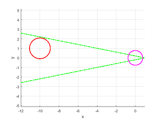
where Δ​t\Delta t is the time-step size, and we set Δ​t=0.2\Delta t=0.2. Figure 4 illustrates the problem setup. The red circle denotes the 3​σ3\sigma error of the initial state distribution of xx and yy coordinates. The magenta circle denotes the 3​σ3\sigma error of the terminal state distribution of xx and yy coordinates. Specifically, the initial condition is

μ0=[−10,1,0,0],Σ0=𝚍𝚒𝚊𝚐⁡(0.1,0.1,0.01,0.01),\mu_{0}=[-10,1,0,0],\qquad\Sigma_{0}=\mathtt{diag}(0.1,0.1,0.01,0.01), (99)

while the terminal constraint is

μN=[0,0,0,0],ΣN=0.5​Σ0.\mu_{N}=[0,0,0,0],\qquad\Sigma_{N}=0.5\Sigma_{0}. (100)

The green dotted lines illustrate the state constraints. Specifically,

15​(x−1)≤y≤−15​(x−1)\frac{1}{5}(x-1)\leq y\leq-\frac{1}{5}(x-1) (101)

The vehicle has to remain in the region between the two lines while moving from the red to the magenta regions. Such a “cone”-shaped constraint is seen in many engineering applications, e.g., the instrument landing for aircraft, spacecraft rendezvous, and drone-landing on a moving platform. The probabilistic threshold for the violation of chance constraints was specified a priori, and we set pj,fail=0.0005p_{j,\rm{fail}}=0.0005.

Refer to caption
Figure 4: Problem setup for the second numerical example.

The objective function is

J⁡(x0,…,xN−1,u0,…,uN−1)=∑k=0N−1xk⊤​Qk​xk+uk⊤​Rk​uk,J(x_{0},\ldots,x_{N-1},u_{0},\ldots,u_{N-1})=\sum_{k=0}^{N-1}x_{k}^{\top}Q_{k}x_{k}+u_{k}^{\top}R_{k}u_{k}, (102)

where

Qk=𝚍𝚒𝚊𝚐⁡(10,10,1,1),Rk=𝚍𝚒𝚊𝚐⁡(103,103),Q_{k}=\mathtt{diag}(10,10,1,1),\qquad R_{k}=\mathtt{diag}(10^{3},10^{3}), (103)

with horizon N=20N=20. This problem is infeasible if we do not control the state covariance. See, for example, Figure 5, which shows the results using only the mean steering controller (32). As the covariance grows, it is impossible to find a feasible solution to this problem that will guarantee the satisfaction of chance constraints.

Refer to caption
Figure 5: Mean steering results.

Before discussing the case with chance constraints, we discuss the case without chance constraints, which is illustrated in Fig. 6. By introducing the covariance steering, the uncertainty of the future trajectory successfully reduced.

Refer to caption
Figure 6: Covariance steering results without chance constraints.

Finally, Fig. 7 illustrates the results of the proposed chance-constrained covariance steering approach. The error ellipse successfully changed its shape to avoid collision with the constraints while maintaining the terminal covariance constraints to be less than the pre-specified state covariance.

Refer to caption
Figure 7: Covariance steering results with chance constraints.

6 Summary

This work has addressed the problem of optimal steering of the covariance for a stochastic linear time-varying system subject to chance constraints in discrete time. We showed that if there are no chance constraints, we can independently design the mean and covariance steering controllers, and we introduced an analytic solution for the mean steering. We also showed that the optimal covariance steering problem with chance constraints can be converted to a convex programming problem. The proposed approach was verified using numerical examples. Future work will investigate the applications of the proposed approach to stochastic model predictive controllers.

References

  • [1] S. Shahrokhi, A. Mahadev, and A. T. Becker, “Algorithms for shaping a particle swarm with a shared control input using boundary interaction,” arXiv preprint arXiv:1609.01830, 2016.
  • [2] A. Vinante, M. Bignotto, M. Bonaldi, M. Cerdonio, L. Conti, P. Falferi, N. Liguori, S. Longo, R. Mezzena, A. Ortolan et al., “Feedback cooling of the normal modes of a massive electromechanical system to submillikelvin temperature,” Physical Review Letters, vol. 101, no. 3, p. 033601, 2008.
  • [3] M. Farina, L. Giulioni, L. Magni, and R. Scattolini, “A probabilistic approach to model predictive control,” in IEEE Conference on Decision and Control, Florence, Italy, Dec. 10–13, 2013, pp. 7734–7739.
  • [4] A. F. Hotz and R. E. Skelton, “A covariance control theory,” in IEEE Conference on Decision and Control, vol. 24, Fort Lauderdale, FL, Dec. 11 – 13, 1985, pp. 552–557.
  • [5] T. Iwasaki and R. E. Skelton, “Quadratic optimization for fixed order linear controllers via covariance control,” in American Control Conference, Chicago, IL, June 24 – 26, 1992, pp. 2866–2870.
  • [6] J.-H. Xu and R. E. Skelton, “An improved covariance assignment theory for discrete systems,” IEEE transactions on Automatic Control, vol. 37, no. 10, pp. 1588–1591, 1992.
  • [7] K. M. Grigoriadis and R. E. Skelton, “Minimum-energy covariance controllers,” Automatica, vol. 33, no. 4, pp. 569–578, 1997.
  • [8] A. Hotz and R. E. Skelton, “Covariance control theory,” International Journal of Control, vol. 46, no. 1, pp. 13–32, 1987.
  • [9] E. Collins and R. Skelton, “A theory of state covariance assignment for discrete systems,” IEEE Transactions on Automatic Control, vol. 32, no. 1, pp. 35–41, 1987.
  • [10] Y. Chen, T. T. Georgiou, and M. Pavon, “Optimal steering of a linear stochastic system to a final probability distribution, Part I,” IEEE Transactions on Automatic Control, vol. 61, no. 5, pp. 1158–1169, 2016.
  • [11] Y. Chen, T. Georgiou, and M. Pavon, “Optimal steering of a linear stochastic system to a final probability distribution, Part II,” IEEE Transactions on Automatic Control, vol. 61, no. 5, pp. 1170–1180, 2016.
  • [12] Y. Chen, T. T. Georgiou, and M. Pavon, “Optimal steering of a linear stochastic system to a final probability distribution, Part III,” IEEE Transactions on Automatic Control, 2018.
  • [13] Y. Chen, “Modeling and control of collective dynamics: From Schrödinger bridges to optimal mass transport,” Ph.D. dissertation, University of Minnesota, 2016.
  • [14] J. Ridderhof and P. Tsiotras, “Uncertainty quantication and control during mars powered descent and landing using covariance steering,” in AIAA Guidance, Navigation, and Control Conference, Kissimmee, FL, Jan. 8 – 12, 2018, p. 0611.
  • [15] E. Schrödinger, Über die Umkehrung der Naturgesetze. Verlag Akademie der Wissenschaften in Kommission bei Walter de Gruyter u. Company, 1931.
  • [16] L. V. Kantorovich, “On the transfer of masses,” in Dokl. Akad. Nauk. SSSR, vol. 37, no. 7-8, 1942, pp. 227–229.
  • [17] A. Halder and E. D. Wendel, “Finite horizon linear quadratic Gaussian density regulator with Wasserstein terminal cost,” in American Control Conference, Boston, MA, July 6 – 8, 2016, pp. 7249–7254.
  • [18] M. Goldshtein and P. Tsiotras, “Finite-horizon covariance control of linear time-varying systems,” in IEEE Conference on Decision and Control, Melbourne, Australia, Dec. 12 –15, 2017, pp. 3606–3611.
  • [19] E. Bakolas, “Optimal covariance control for stochastic linear systems subject to integral quadratic state constraints,” in American Control Conference, Boston, MA, July 6 – 8, 2016, pp. 7231–7236.
  • [20] ——, “Optimal covariance control for discrete-time stochastic linear systems subject to constraints,” in IEEE Conference on Decision and Control, Las Vegas, NV, Dec. 12 – 14, 2016, pp. 1153–1158.
  • [21] ——, “Finite-horizon covariance control for discrete-time stochastic linear systems subject to input constraints,” Automatica, vol. 91, pp. 61–68, 2018.
  • [22] A. Geletu, M. Klöppel, H. Zhang, and P. Li, “Advances and applications of chance-constrained approaches to systems optimisation under uncertainty,” International Journal of Systems Science, vol. 44, no. 7, pp. 1209–1232, 2013.
  • [23] M. Farina, L. Giulioni, and R. Scattolini, “Stochastic linear model predictive control with chance constraints - a review,” Journal of Process Control, vol. 44, pp. 53 – 67, 2016.
  • [24] A. Mesbah, “Stochastic model predictive control: An overview and perspectives for future research,” IEEE Control Systems, vol. 36, no. 6, pp. 30–44, 2016.
  • [25] M. Ono, L. Blackmore, and B. C. Williams, “Chance constrained finite horizon optimal control with nonconvex constraints,” in American Control Conference, Baltimore, MD, June 30 – July 2, 2010, pp. 1145–1152.
  • [26] D. S. Bernstein, Matrix Mathematics: Theory, Facts, and Formulas, 2nd ed., 2009, vol. 41.
  • [27] L. Blackmore and M. Ono, “Convex chance constrained predictive control without sampling,” in AIAA Guidance, Navigation, and Control Conference, Chicago, IL, Aug. 10 – 13, 2009, p. 5876.
  • [28] A. Prékopa, “Boole-Bonferroni inequalities and linear programming,” Operations Research, vol. 36, no. 1, pp. 145–162, 1988.
  • [29] L. Blackmore, M. Ono, and B. C. Williams, “Chance-constrained optimal path planning with obstacles,” IEEE Transactions on Robotics, vol. 27, no. 6, pp. 1080–1094, 2011.
  • [30] A. Carvalho, Y. Gao, S. Lefevre, and F. Borrelli, “Stochastic predictive control of autonomous vehicles in uncertain environments,” in International Symposium on Advanced Vehicle Control, Tokyo, Japan, Sept. 22–26, 2014.
  • [31] M. Grant and S. Boyd, “CVX: Matlab software for disciplined convex programming, version 2.1,” http://cvxr.com/cvx, Mar. 2014.
  • [32] MOSEK ApS, The MOSEK optimization toolbox for MATLAB manual. Version 8.1., 2017. [Online]. Available: http://docs.mosek.com