Path to Stochastic Stability: Comparative Analysis of Stochastic Learning Dynamics in Games
Abstract
Stochastic stability is a popular solution concept for stochastic learning dynamics in games. However, a critical limitation of this solution concept is its inability to distinguish between different learning rules that lead to the same steady-state behavior. We address this limitation for the first time and develop a framework for the comparative analysis of stochastic learning dynamics with different update rules but same steady-state behavior. We present the framework in the context of two learning dynamics: Log-Linear Learning (LLL) and Metropolis Learning (ML). Although both of these dynamics have the same stochastically stable states, LLL and ML correspond to different behavioral models for decision making. Moreover, we demonstrate through an example setup of sensor coverage game that for each of these dynamics, the paths to stochastically stable states exhibit distinctive behaviors. Therefore, we propose multiple criteria to analyze and quantify the differences in the short and medium run behavior of stochastic learning dynamics. We derive and compare upper bounds on the expected hitting time to the set of Nash equilibria for both LLL and ML. For the medium to long-run behavior, we identify a set of tools from the theory of perturbed Markov chains that result in a hierarchical decomposition of the state space into collections of states called cycles. We compare LLL and ML based on the proposed criteria and develop invaluable insights into the comparative behavior of the two dynamics.
I Introduction
Stochastic learning dynamics, like log-linear learning, address the issue of equilibrium selection for a class of games that includes potential games (see, e.g., [1], [2], [3] and [4]). Because of the equilibrium selection property, these learning dynamics have received significant attention, particularly in the context of opinion dynamics in coordination games (see, e.g., [2] and [5]) and game theoretic approaches to the distributed control of multiagent systems [6].
A well-known problem of stochastic learning dynamics is the slow mixing of their induced Markov chain [2], [7], [8]. The mixing time of a Markov chain is the time required by the chain to converge to its stationary behavior. This mixing time is crucial because the definition of a stochastically stable state depends on the stationary distribution of the Markov chain induced by a learning dynamics. The slow mixing time implies that the behavior of these dynamics in the short and medium run are equally important particularly for engineered systems with a limited lifetime. However, stochastic stability only deals with the steady-state behavior and provides no information about the transient behavior of these dynamics.
The speed of convergence of stochastic learning dynamics is an active area of research that is receiving significant research attention [9], [10], [11], [12], [13], and [14]. However, there is another aspect related to the slow convergence of these dynamics that has received relatively little research attention. Stochastic stability only explains the steady-state behavior of a system under a learning rule. We establish that there are learning dynamics with considerably different update rules that lead to the same steady-state behavior. Since these learning dynamics have the same stochastically stable states, stochastic stability cannot distinguish between these dynamics. The different update rules may result in significantly different behaviors over short and medium run that may be desirable or undesirable but remain entirely unnoticed.
We first establish the implications of having different learning rules with the same steady state. Through an example setup, we demonstrate the differences in short and medium run behaviors for two particular learning dynamics with different update rules that lead to the same stochastically stable states. The example setup is that of sensor coverage game in which we formulate a sensor coverage problem in the framework of a potential game. An important conclusion that we draw from this comparison is that for stochastic learning dynamics, characterization of stochastically stable states is not sufficient. It is also essential to analyze the paths that lead to these stochastically stable states from any given initial condition. Analysis of these paths is critical because there are specific properties of these paths that play a crucial role not only in the short and medium run but also in the long run steady state behavior of the system.
The transient behavior of stochastic dynamics was studied in the context of learning in games in [15] and [16]. However, the issues related to various learning dynamics leading to the same steady state behavior were not highlighted in these works. Therefore, after motivating the problem, we propose a novel framework for performing a comparative analysis of different stochastic learning dynamics with the same steady state. The proposed framework is based on the theory of Markov chains with rare transitions [17], [18], [19], [20], [21], [22], and [23].
In the proposed framework, we present multiple criteria for comparing the short, medium, and long-run behaviors of a system under different learning dynamics. We refer to the analysis related to the short-run behavior as first order analysis. The first order analysis deals with the expected hitting time of the set of pure Nash equilibria, which is the expected time to reach a Nash equilibrium (NE) for the first time. Because of the known hardness results of computing a NE [24], [25], and the fact that all the Nash equilibria of a potential game are not necessarily potential maximizer, the first order analysis is typically not considered for stochastic learning dynamics. However, we are interested in the comparative analysis of learning dynamics for which we show that first-order analysis provides valuable insights into the behavior of a system.
We refer to the analysis related to the medium and long-run behavior of stochastic learning dynamics as higher-order analysis. The higher-order analysis is based on the fact that the Markov chains induced by stochastic learning dynamics explore the space of joint action profiles hierarchically. This hierarchical exploration of the state space is well explained by an iterative decomposition of the state space into cycles of different orders as shown in [17], [19], [18], and [26]. Thus, the evolution of Markov chains with rare transitions can be well approximated by transitions among cycles of proper order.
Therefore, we develop our higher order analysis on the cycle decomposition of the state space as presented in [27]. We compare the behavior of different learning rules by comparing the exit height , and the mixing height of the cycles generated by the cycle decomposition algorithm applied to these learning rule. The significance of these parameters is that once a Markov chain enters a cycle, the time to exit the cycle is of the order of and the time to visit each state within a cycle before exiting is of the order of . Thus, we can efficiently characterize the behavior of each cycle from and .
Our comparative analysis framework applies to the class of learning dynamics in which the induced Markov chains satisfy certain regularity conditions. However, we present the details of the framework in the context of two particular learning dynamics, Log-Linear Learning (LLL) and Metropolis Learning (ML) over potential games. Log-Linear learning is a noisy best response dynamics in which the probability of a noisy action from a player is inversely related to the cost of deviating from the best response. This learning rule is well-known in game theory and the stationary distribution of the induced Markov chain is a Gibbs distribution, which depends on a potential function. The Gibbs distribution over the space of joint action profiles assigns the maximum probability to the action profiles that maximize the potential function. Moreover, it was shown in [28] that LLL is a good behavioral model for decision making when the players have sufficient information to compute their utilities for all the actions in their action set given the actions of other players in the game.
On the other hand, Metropolis learning is a noisy better response dynamics for which the induced Markov chain is a Metropolis chain. It is well established in the statistical mechanics literature that the unique stationary distribution of Metropolis chain is the Gibbs distribution (see, e.g., [18] and [20]). As a behavioral model for decision making, ML is related closely to the pairwise comparison dynamics presented in [29]. Thus, ML is a behavioral model for decision making with low information demand. A player only needs to compare its current payoff with the payoff of a randomly selected action. It does not need to know the payoffs for all the actions as in LLL. The only assumption is that each player has the ability or the resources to compute the payoff for one randomly selected action.
Hence, we have two learning dynamics, LLL and ML, which correspond to two behavioral models for decision making with very different information requirements. However, both of the learning rules lead to the same steady-state behavior. We compare these learning dynamics based on the proposed framework. The crux of our comparative analysis is that the availability of more information in the case of LLL as compared to ML does not guarantee better performance when the performance criterion is to reach the potential maximizer quickly.
A summary of our main contributions in this work is as follows
Contributions
- •
For problem motivation, we present our setup of sensor coverage game in which we formulate the sensor coverage problem with random sensor deployment as a potential game.
- •
For the first order analysis, we derive and compare upper bounds on the expected hitting time to the set of NE for both LLL and ML.
- •
We also obtain a sufficient condition to guarantee a smaller expected hitting time to the set of Nash equilibria under LLL than ML from any initial condition.
- •
For higher order analysis, we identify cycle decomposition algorithm as a useful tool for the comparative analysis of stochastic learning dynamics. Moreover, we show through an example of a simple Markov chain that cycle decomposition algorithm is also suitable for describing system behavior at different levels of abstraction.
- •
We compare the exit heights and mixing heights of cycles under LLL and ML. We show that if a subset of state space is a cycle under both LLL and ML, then the mixing and exit heights of that cycle will always be smaller for ML as compared to LLL.
II Background
II-A Preliminaries
We denote the cardinality of a set by . For a vector , denotes its entry and is its Euclidean norm. The Hamming distance between any two vectors and in is
| (1) |
denotes the dimensional probability simplex, i.e.,
where is a column vector in with all the entries equal to 1.
II-B Markov Chains
A discrete time Markov chain on a finite state space is a random process that consists of a sequence of random variables such that for all and
where and for all . Let be the transition matrix for Markov chain and be the transition probability from state to . A distribution is a stationary distribution with respect to if
If a Markov chain is ergodic and reversible, then it has a unique stationary distribution, i.e.,
for all . The following definitions are adapted from [2].
Definition II.1
Let be a transition matrix for a Markov chain over state space . Let be a family of perturbed Markov chains on for sufficiently small corresponding to . We say that is a regular perturbation of if
- 1.
is ergodic for sufficiently small ,
- 2.
, and
- 3.
for some implies that there exists some function such that
where is the cost of transition from to and is normally referred to as resistance.
The Markov process corresponding to is called a regularly perturbed Markov process.
Definition II.2
Let be a regular perturbation of with stationary distribution . A state is a stochastically stable state if
Thus, any state that is not stochastically stable will have a vanishingly small probability of occurrence in the steady state as .
Given any two states and in , is reachable from if for some . The neighborhood of is
A path between any two states and in is a sequence of distinct states such that , , , and for all . The length of the path is denoted as . The superscript will be ignored in path notation when the state space is clear from the context. Given a set and a path , we say that if for all . We define as the set of all paths between states and in state space . States and communicate with each other () if the sets and are not empty.
Definition II.3
A set is connected if for every , .
Definition II.4
The hitting time of is the first time it is visited, i.e.,
The hitting time of a set is the first time one of the states of is visited, i.e.,
Definition II.5
The exit time of a Markov chain from is , where
where . We will refer to as the boundary of . In the above definition it is assumed that .
II-C Game Theory
Let be a set of strategic players in which each player has a finite set of strategies . The utility of each player is represented by a utility function where is the set of joint action profiles. The combination of the action of the player and the actions of everyone else is represented by . The joint action profiles of all the players except are represented by the set
Player prefers action profile over , where and , if and only if . If , then it is indifferent to both the actions. An action profile is a Nash Equilibrium (NE) if
for all and . The best response set of player given an action profile is
The set of all possible best responses from an action profile is
The neighborhood of an action profile is
The agent specific neighborhood set of action profile is
Potential Game: A game is a potential game if there exists a real valued function such that
for all and for all , . The function is called a potential function.
III Stochastic Learning Dynamics
Stochastic learning dynamics is a class of learning dynamics in games in which the players typically play best/better reply to the actions of other players. However, the players sporadically play noisy actions for exploration because of which these dynamics have equilibrium selection property for a class of games like potential games.
III-A Log-Linear Learning
Let be the joint action profile representing the current state of the game. Then, the steps involved in LLL are as follows.
- 1.
Activate one of the players, say player , uniformly at random.
- 2.
All other players repeat their previous actions.
- 3.
Player selects an action with the following probability
(2) Here is a normalizing constant, is a best response of player to , and
In (2), is the noise parameter, normally referred to as temperature. For , the players update their strategies uniformly at random. However, as , the probability of the actions yielding higher utilities increases.
Thus, LLL induces a Markov chain over the joint action profile with transition matrix . The transition probability between any two distinct action profiles and is
It was shown in [30] that for LLL is a regular perturbation of with . That is why we have used the notation instead of . Here, is the transition matrix of the Markov chain induced by sequential best response dynamics. It was also proved in [30] that in an -player potential game with a potential function , if all the agents update their actions based on LLL, then the only stochastically stable states are the potential maximizers. The stationary distribution for is the Gibbs distribution
| (3) |
where is the normalizing constant.
III-B Metropolis Learning
We introduce another learning dynamics that has the same stationary distribution as in (3). We refer to it as Metropolis Learning (ML) because the Markov chain induced by ML is a Metropolis chain, which is well studied in statistical mechanics and in simulated annealing [20]. The steps involved in ML are as follows.
- 1.
Activate one of the players, say player , uniformly at random.
- 2.
All other players repeat their previous actions.
- 3.
Player selects an action uniformly at random.
- 4.
Player switches its action form to with probability
Thus, the probability of transition from to is
| (4) |
where if and is equal to zero otherwise.
In ML, player switches to a randomly selected action with probability one as long as . Here, is the action that player was playing in the previous time slot. Thus, unlike LLL in which a player needs to compute the utilities for all the actions in its action set given , the update in ML only requires a player to make a pairwise comparison between a randomly selected action and its previous action. Furthermore, the probability of a noisy action is a function of loss in payoff as compared to the previous action.
Metropolis learning generates a Markov Chain over joint action profile with transition matrix . The transition probability between any two distinct action profiles and is
Next we show that is a regularly perturbed Markov process.
Lemma III.1
Transition matrix is a regular perturbation of , where is the transition matrix for asynchronous better reply dynamics. Moreover, the resistance of any feasible transition from to is
| (5) |
Proof:
To prove that is a regular perturbation, we first describe the unperturbed process which is asynchronous better reply dynamics. The unperturbed process has the following dynamics.
- 1.
A player, say , is selected at random.
- 2.
All the other players repeat their previous actions.
- 3.
Player selects an action uniformly at random.
- 4.
Player switches its action from to if
Otherwise, it repeats . Thus
Similar to LLL, the noise parameter . The Metropolis chain is ergodic for a given and it satisfies . For the final condition
where for any given pair and . Thus, is a regular perturbation of . ∎
The important fact regarding ML in the context of this work is that the stationary distribution is also the Gibbs distribution, i.e.,
| (6) |
Thus, from the perspective of stochastic stability, both LLL and ML are precisely the same. To observe and understand the effects of different update rules on system behavior, we simulated a sensor coverage game with both LLL and ML. Next, we present the setup and the results of the simulation.
IV Motivation: Sensor Coverage Problem
To study the difference in behaviors between LLL and ML, which is ignored under stochastic stability, we set up sensor coverage problem as a potential game. Through extensive simulations under various noise conditions, we exhibit the essential differences between the behavior of these learning dynamics in the short and medium runs. We want to mention here that this formulation of sensor coverage problem with random sensor deployment in a potential game theoretic framework is also a contribution and can be of independent interest in the context of local scheduling schemes for sensor coverage problem.


IV-A Coverage Game Setup
Consider a scenario in which sensors are deployed randomly to monitor an environment for a long period of time. We approximate with a square region defined over intervals . To simplify the problem, the area is discretized as a 2-dimensional grid represented by the Cartesian product . The location of each sensor is where , i.e., is a random variable uniformly distributed over the region of interest . The footprint of sensor is a circular disk of radius , i.e.,
We assume that each sensor can choose the radius of its footprint from a finite set, which determines its energy consumption. Let be the communication range of each sensor. We assume that , where is the maximum sensing radius.
We propose a game-theoretic solution to the sensor coverage problem in which we formulate the problem as a strategic game and implement some local learning rule so that each sensor can learn its schedule based on local information only. The players in this game are the sensors and each player has actions, i.e., and . Here, an action of a player is its sensing radius. For each sensor, , which is the off state of a sensor. The joint action profile is the joint state of all the sensors.
Let be a point on the grid where . The state of a grid point is whether it is covered or uncovered, i.e.,
Thus, the objective is to solve the following optimization problem.
where
is the total coverage achieved by the sensor network and
is the total cost incurred by the sensors that are on. We assume that , i.e., no cost is incurred by the sensors that are off.
The local utility of each player is computed through marginal contribution utility as explained in [31] with base action , i.e., the base action of each sensor is to be in the off state in which there is no energy consumption. If is the joint state of all the other sensors, then the utility of player for action is
The above equation implies that . For any
Thus, the marginal contribution utility of sensor with action is the number of grid points that are covered by the sensor exclusively with footprint of radius minus the cost .
To make the payoff and the cost terms in compatible, we express the cost of turning a sensor on as a function of the minimum number of grid points that a sensor should cover exclusively. Let be the maximum number of grid points that a sensor can cover if its footprint has radius . We define the cost as
Thus, the net utility of a sensor is negative if the number of points it covers exclusively is less than given .
IV-B Simulation Results
We simulated the sensor coverage game with , , , and for all . For this setup, the maximum global utility was
which was computed numerically based on extensive simulations. To achieve the maximum payoff, we implemented LLL and ML with different values for the noise parameter and the number of iterations . The results of the simulation are presented in Figs. 1 and 2.
Initially, all the sensors were in the off state. To compare the short-term behavior of the network with small noise, we set and ran the simulation for twenty times for both LLL and ML with . Since players were randomly selected to update their actions at each decision time, each simulation led to a different system configuration in one hundred iterations even with the same initial condition. The results of twenty simulations are presented in Fig. 1. In Fig. 1(a), we show the number of iterations to reach a NE for the first time under LLL and ML. Based on the results in Fig. 1(a), the average number of iterations to reach a NE for the first time under LLL and ML were 43.15 and 63.75 respectively. Thus, on average, the system reached a NE faster under LLL than ML.
For a system with multiple Nash equilibria, reaching a NE faster is not the only objective. The quality of the NE is also a significant factor. In Fig. 1(b), we present the global payoff at the Nash equilibria reached under LLL and ML in our twenty simulations. The global payoffs at the Nash equilibria under LLL and ML had a mean value of 229.6 and 230.1, and a standard deviation of 8.39 and 12.49 respectively. Although the average global payoffs were almost equal, the higher standard deviation under ML implies that ML explored the state space more as compared to LLL. As of result of this higher exploration tendency, the system achieved the global maximum of 247 three times under ML and only one time under LLL.
Thus, based on the comparisons from Fig. 1, LLL seems to be better than ML because it can lead to a NE faster on average. However, ML seems to have a slight edge over LLL if we consider the quality of the Nash equilibria. This observation provides a strong rationale for comprehensive comparative analysis because we cannot simply declare one learning rule better than the other.
For higher order analysis, the objective was to observe and compare system behavior over an extended period. For comparison, we were interested in the following crucial aspects.
- •
Time to reach a payoff maximizing NE under each learning dynamics.
- •
The paths adopted to reach the payoff-maximizing NE and their characteristics.
- •
System behavior after reaching a payoff maximizing NE.
Therefore, we simulated the system for iterations with and , and for iterations with . The results are presented in Figs 2(a)-2(c) respectively.
For , optimal configuration could not be achieved under both LLL and ML even in iterations. For LLL, the network remained stuck at some NE for iterations. Under ML, there was a single switch in network configuration after approximately from one NE to another. As we increased the noise to , payoff maximizing configurations were reached under both LLL and ML. However, the number of iterations to reach these optimal configurations were huge, particularly in LLL. Finally, for , the optimal configurations were reached rapidly.
The ability of ML to stay at an optimal configuration after reaching it is affected more by noise as compared to LLL. In Fig. 2(a) with , the network configuration switched from one NE to another under ML, but there was no switch under LLL. In Fig. 2(b) with , the network configuration switched to an optimal NE quickly under ML then under LLL. Finally, the increase of noise led to an interesting behavior that can be observed in Fig. 2(c). Under ML, the network configuration kept on leaving the payoff-maximizing configurations periodically for a significant duration of times. However, under LLL, after reaching an optimal configuration, the network never left the configuration for long durations of time. Every time it left the optimal configuration because of noise, it immediately switched back. We can summarize the observations from the simulation setup as follows
- 1.
In short run, LLL can drive network configuration to a NE quickly as compared to ML.
- 2.
In short, medium, and long run, starting from the same initial condition, LLL and ML can drive network configurations along entirely different paths that lead to the payoff-maximizing configurations in the long run.
- 3.
The effect of noise on LLL and ML is significantly different.
From the above observations, we can conclude that the concept of stochastic stability alone is not sufficient to describe the behavior of stochastic learning dynamics. However, these observations are based on the simulation of a particular system under certain conditions, which prohibits us from drawing any general conclusions regarding the behavior of these learning rules. Therefore, we present a general framework to analyze and compare the behavior of different learning rules that have the same stochastically stable states. We establish that the setup of Cycle Decomposition is useful for the comparative analysis of learning dynamics in games. In particular, we identify and compare the parameters that enable us to explain the system behavior that we observed in the motivating setup of sensor coverage games.
V Cycle Decomposition
Consider a Markov chain on a finite state space with transition matrix . We assume that the transition matrix satisfies the following property.
| (7) |
where for and
| (8) |
Here is defined as follows
For any pair, can be considered as a transition cost from to . It is assumed that the function is irreducible, which implies that for any state pair , there exists a path of length such that
Definition V.1
A function is induced by a potential function if, for all and in , the following weak reversibility condition is satisfied.
| (9) |
The following result is from [32] (Prop. 4.1).
Proposition V.1
Thus, in the limit as , only the states maximizing the potential will have a non-zero probability. Based on Prop. V.1, there is an entire class of Markov chains that lead to potential maximizers. We want to mention here that the results in [32] were for minimizing a potential function. Since we are dealing with maximizing a payoff, all the definitions and results are adapted accordingly.
V-A Cycle Decomposition Algorithm
Cycle Decomposition Algorithm (CDA) was presented in [26], based on the ideas originally presented in [17]. It was presented to study the transient behavior of Markov chains that satisfy (7), (8), and (9) and lead to the stationary distribution defined in Prop. V.1. In this algorithm, the state space is decomposed into unique cycles in an iterative procedure. The formal definition of cycle as presented in [32] and [21] is as follows
Definition V.2
A set is a cycle if it is a singleton or it satisfies either of the two conditions.
- 1.
For any , in ,
- 2.
For any , in ,
where is the number of round trips including and performed by the chain before leaving .
The first condition simply means that a subset is a cycle if starting from some , the probability of leaving before visiting every state is exponentially small. Thus,
The second statement states that the expected number of times each is visited by starting from any is exponentially large.
For higher order comparative analysis, we first decompose the state space into cycles via CDA. Then, we compare the properties of the cycles under each learning dynamics. For the completeness of presentation, we reproduce CDA in Alg. 1. The outcome of CDA as presented in Alg. 1 is the set defined in (12). To explain system behavior using CDA, we need the following definitions and results, which are mostly adopted from [26].
The minimum cost of leaving a state is
We will refer to as the exit height of state . For any set of states and such that , we define
i.e., is the excess cost above the minimum transition cost form . For a path
The exterior boundary of set is
The interior boundary of set is
We say that a cycle is non-trivial if it has a non-zero exit height. Thus, a singleton is non-trivial cycle if it is a local maxima. The order of the decomposition of the state space is
An increasing family of cycles is defined for each as follows. Define . For each
| (10) |
Given a set such that , the maximal proper partition is
where .
For a cycle ,
- •
order is
- •
exit height is
- •
mixing height is
- •
potential is
- •
communication altitude between any two states and is
where is the element in the path .
- •
the communication altitude of a cycle is
| (11) |
| (12) |
The exit and the mixing heights of a cycle provides an estimate of how long the Markov chain will remain in the cycle. The potential of a cycle is the maximum potential of a state within the cycle. The communication altitude was introduced in [26], and it was shown that relates , and as follows.
| (13) |
for any . Another important result form Prop. 2.16 in [26] is
| (14) |
where is the smallest cycles containing both and . The definition of is adjusted because we are maximizing a utility instead of minimizing a cost. However, all the results from [26] remain valid, and play an important role in the comparative analysis of LLL and ML.
Theorem V.1
Let . For any and for any and in
| (15) | ||||
| (16) |
as the noise parameter , where is the exit time of from and is the hitting time for .
Eq. (15) implies that the exit time of a Markov chain from a cycle starting from any is proportional to the exit height of . Moreover, (16) suggests that before leaving the cycle , will visit all the states within exponentially large number of times. Eqs. (15) and (16) enable us to explain the behavior of a Markov chain from its cycles. In the next section, we apply Cycle decomposition to ML and LLL and demonstrate the effectiveness of our proposed approach in explaining the behavior of the corresponding evolutionary process.
VI Cycle Decomposition For ML And LLL
Before we can carry out comparative analysis using CDA, we need to establish that both ML and LLL satisfy the criteria for CDA. The state space for these learning rules is the set of joint action profiles , where . We define
Proof:
To prove this result, we need to show that there exist cost and functions for both ML and LLL that satisfy the three equations in the above statement. We begin with Metropolis learning. Given any pair of distinct action profiles and in , we define
| (17) |
where is the maximum number of actions of any player in the game. It is straightforward to verify that
and and satisfy (7).
Next, we show that is induced by a potential function . Given any two action profile and , two cases need to be considered. The first case is when , which implies . Thus, both the left and right sides of (9) are equal to . The second case is when . In this case, the action profiles can be written as , . Rearranging (9)
where
For potential games
Thus, is induced by a potential function, which concludes the proof for ML.
For any given action profile pair and such that ,
Moreover, and as defined above, satisfy (7). For the weak reversibility condition,
By following the same series of arguments as for ML, we conclude that is induced by a potential function , which concludes the proof. ∎
Proposition VI.1 is restricted to LLL and ML. We rewrite (7) as
By comparing the above inequalities with Def. II.1, we can easily verify that for and for every pair, any regularly perturbed process satisfies (7) and (8). Moreover, if the game is a potential game, then it satisfies (9). Thus, the framework of cycle decomposition applies to any stochastic learning dynamics on potential games that generate a regularly perturbed Markov process. The condition of is not strict and (7) can easily be expressed with a general noise parameter . Since both LLL and ML have , we will not go into the details. Thus, from this point onward, we will use the terms cost and resistance for interchangeably.


VI-A Stochastic Learning Dynamics Explained by CDA
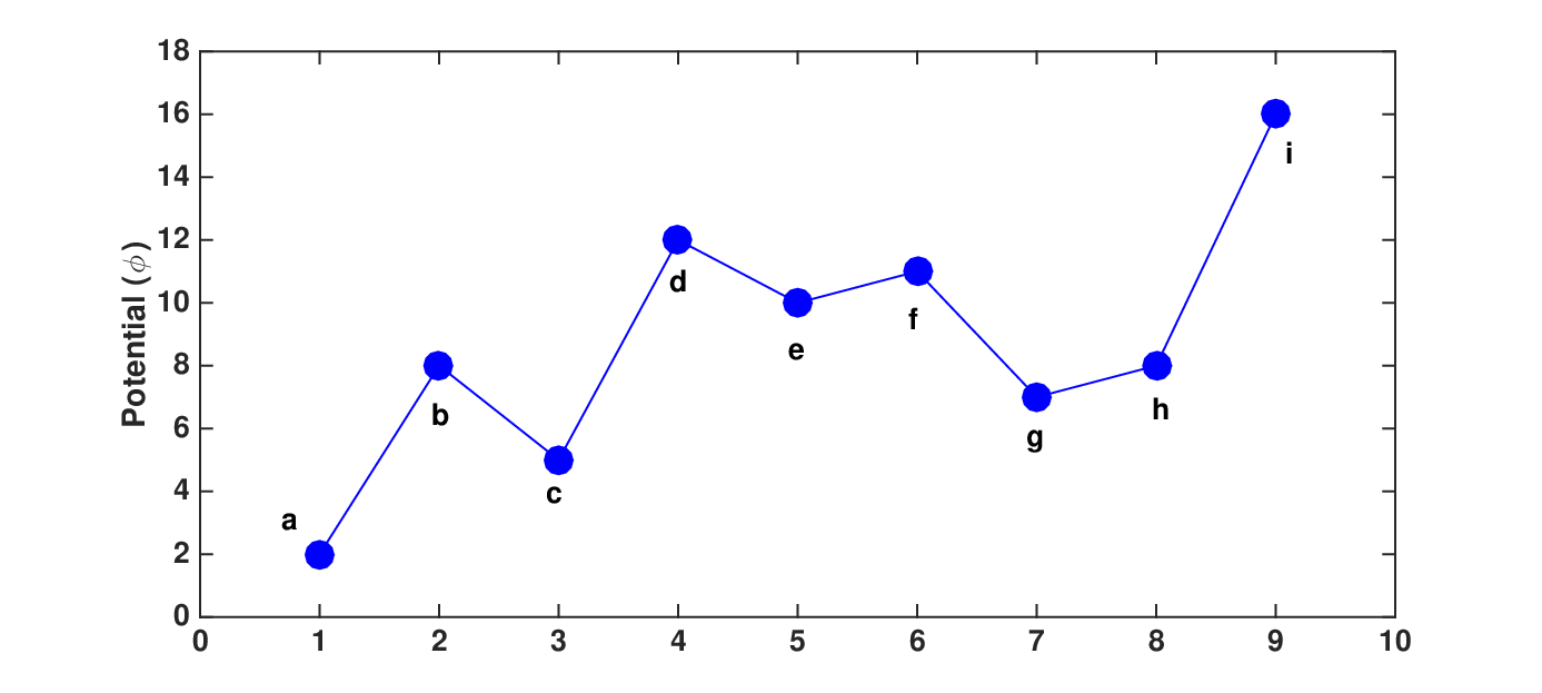
In the previous section, we proved that CDA applies to both ML and LLL. Next, we establish that CDA can effectively explain the medium and long run behaviors of stochastic learning dynamics through a simple example. We consider a Markov chain over state space . The possible transitions between the states and the energy landscape over the entire state space are presented in Fig. 3(a). This Markov chain is selected to explain the working and effectiveness of CDA and is not assumed to be associated with any particular game.
The outcomes of first iterations of CDA for ML are depicted in Figs. 3(b)-3(e). The final iteration results in a single cycle containing the entire state space. The only information conveyed by the last level is that the chain is irreducible, which is already known. Therefore, we start from as presented in Fig. 3(e). The set comprises a singleton with , and a non-trivial cycle of order three, containing all the remaining states with exit height of 14. Based on this level and Thm. V.1, we can deduce that if the initial condition is , the Markov chain will leave this state quickly as the noise parameter , and will hit a large cycle containing all the other states. This cycle has an exit height of 14, which implies that the time to exit from this cycle will be proportional to . Moreover, the chain will visit all the states within this big cycle an exponential number of times before exiting. Therefore, for a system with a finite lifetime and initial condition , we can safely conclude that the system will leave quickly and will never revisit it for all practical purposes.
However, what happens when the chain leaves or if the initial condition is not in ? These questions cannot be answered adequately from . To answer these questions, we need to go one level lower to the output of the second iteration . Graph demonstrates that the non-trivial cycle in is composed of a singleton , one non-trivial cycle of order zero and exit height three, and another non-trivial cycle of order two and exit height 11.
Graph offers more details about the behavior of the Markov chain as compared to . It reveals that after exiting from , the Markov chain will hit where it will get stuck for a time proportional to . On exiting , the chain will hit with high probability as because the transition from to is the transition of minimum cost from . From , the chain can either return to , or move on to with equal probabilities. However, once it hits , it will stay within this cycle for most of the time because the exit height of this cycle is 11 which is more than three times the exit height of . Thus, we can conclude from that in the long run, the Markov chain will spend most of its time within the cycle after the short and medium run behavior described above.
Similarly, we can explain the behavior within by examining presented in Fig. 3(c). Although switching form to furnished more information, there is one drawback. Given that the Markov chain is at a state other than , we cannot easily approximate the hitting time of from . Similarly, switching from to can provide more information about the behavior of the chain restricted to the set of states . However, we can lose high-level information about the transition behavior between and the other states in the state space. Thus, switching from the output of a high-level iteration to a low-level iteration of CDA delivers information of higher resolution. However, this high-resolution information is restricted to small subsets of state space. On the other hand, moving from a lower level to a higher level of CDA yields high-level details on transitions from one set of states to another set of states but abstracts away low-level information.
Regardless of which level of CDA we are analyzing, the key parameter that enables us to describe system behavior through CDA is the exit height of a cycle, which depends on the mixing height of that cycles according to (11). To verify this claim, we apply CDA under LLL on the chain in Fig.3(a), and compare the output with output under ML discussed before. The outputs of the first iteration under ML and the second iteration under LLL are presented in Fig. 4. The first observation is that both the graphs have the same cycles but different transition costs. The difference in transition costs is highlighted in the figure with a different color.
Assuming that is the initial condition, both the dynamics have the same behavior till the chain reaches the state . At , ML can transition to or with equal probability. However, LLL will transition to with high probability since the transition to has a high cost. Thus, LLL will hit the cycle faster as compared to ML. However, the exit height of this cycle under LLL is six which is one unit higher than the exit height under ML. The difference in exit heights implies that although ML will reach late, it has the ability to leave this cycle quickly as compared to LLL. After exiting from , both the chains will hit the state . From the state , ML can transition back to or to with equal probability, where state is the potential maximizer. However, LLL will return to with high probability because the transition cost to is high. This comparative analysis of the chain in Fig. 3(a) revealed that if is the initial condition LLL will initially proceed towards the potential maximizer faster as compared to ML. However, it can get stuck in a cycle longer than ML. Moreover, ML has a zero cost path to potential maximizer from whereas no such path exists for LLL.
The comparison of LLL and ML based on Fig. 4 signifies the importance of the qualities of the paths that lead to a stochastically stable state from any given initial condition. Furthermore, it highlights the importance of exit height in explaining system behavior. Thus, for comparative analysis, we will compare the mixing and exit heights of cycles under ML and LLL. In this work, the comparison is restricted to subsets of state space that are cycles under both LLL and ML.
VII Comparative Analysis of ML and LLL
In this section, we present the main results of this work related to the comparative analysis of stochastic learning dynamics in games. Although the results are presented in the context of LLL and ML, the techniques can be extended to any learning dynamics that satisfy the criteria in (7), (8), and (9). We divide the comparative analysis into first order and higher order analysis.
VII-A First Order Analysis
In the first order analysis, we compare the expected hitting times to the set of Nash equilibria for both the learning rules. We first derive upper bounds on the expected hitting times to the set of Nash equilibria and present a comparative analysis of these bounds. Then, we determine a sufficient condition to guarantee that the expected hitting time to the set of Nash equilibria will be smaller for LLL then ML from any given initial action profile. For analysis purposes, we assume that for any action profile pair and such that
| (19) |
This is not a restrictive assumption and is placed for simplifying the analysis. Otherwise, if and , we can simple merge and into a single state.
Let be the set of all the Nash equilibria in , and let be the hitting time to under a learning rule where . Given any path , let
Here is the probability that the Markov chain moves along the path under learning dynamics . From (7),
We define

i.e., is the set of zero cost paths from action profile to under . The set of zero cost paths from any initial condition is
Let
where is the length of the longest paths from to under and is the length of the shortest paths from to under . Before presenting the main results, we need to prove the following propositions.
Proposition VII.1
If an action profile , then and are non-empty for a finite state space .
Proof:
The result is proved for LLL because the proof for ML is exactly the same. We establish that is non-empty by showing that we can always construct a path that belongs to this set.
Let . Assume that there does not exist any such that . This will imply that , which is a contradiction. Thus, there exists an action profile such that . Define . If , we are done and . If , we can argue in the same manner as before that there exists an action profile such that . Define . By repeating this argument times, we obtain
The condition in (19) implies that for all . Thus, all the action profiles in the path are unique. The uniqueness of the elements of ensures that this process terminates in finite number of steps, say , since has finite number of elements. Then ∎The argument of ML is exactly the same. In fact, Prop. VII.1 is valid for any Markov chain that satisfies Eqs. (7).
Proposition VII.2
For LLL and ML, .
Proof:
For any pair of distinct action profiles and
but the converse is not true. To prove this statement, let and be two action profiles in . If , then , i.e., is a best response of player to . Thus,
To show that the converse is not true, let , which implies that . However, if then . Thus, given an action profile , all the zero cost paths from to under LLL are also zero cost paths under ML. However, a zero cost path in ML does not necessarily has zero cost under LLL, which concludes the proof. ∎
Proposition VII.3
The functions satisfying (7) for LLL and ML have the following relation
| (20) |
Proof:
Recall from (17) and (18) that
For any player and any action profile
Thus, , which concludes the proof. ∎
Next, we present our first result for the first order comparative analysis.
Theorem VII.1
There exists constants and that lie in the interval such that
such that . Here is the integer part of the real number .
Proof:
Let be a non-negative continuous random variable. Then, the expected value of is
To prove (VII.1), we will first compute point-wise upper bounds for the probabilities
and show that the computed bounds are integrable. Then, we will use the fact that if and are integrable functions over the interval , then
implies
We begin the proof with LLL. From Prop. VII.1 we know that given any initial condition, there exists a path of zero cost in the set with length less than or equal to , where
In the above expression is the length of the shortest zero cost path from to . Thus, for , the following holds
where is a lower bound on the probability of moving along a zero cost path of length . Thus, for any ,
By setting
we get the desired result, where is the maximum of the minimum path lengths from any initial condition in .
We repeat the same steps for ML. For any initial condition, there always exists a zero cost path to under ML of length less than or equal to , where
Therefore, for ,
For any , the above inequality leads to
where
yields the desired result.
The function
is monotonically decreasing and is bounded from below by zero for . Therefore, the integrals in (VII.1) are bounded, which concludes the proof for (VII.1).
Finally, we prove that . From Prop. VII.2, every zero cost path to under LLL is also a zero cost path to under ML. Moreover, the number of zero cost paths from any initial condition to under ML is always greater than or equal to the corresponding number of paths under LLL. Thus, for any initial condition , there can exist paths of shorter lengths in than the paths in , which implies
Therefore,
which concludes the proof of Thm. VII.1. ∎
We can develop interesting insights into the behavior of LLL and ML from the results in Thm. VII.1. The upper bounds on the expected hitting times to the set of Nash equilibria in (VII.1) depend on two parameters and for . We have already proved that because there can be paths of shorter lengths to the set under ML then LLL. This inequality favors ML in the context of expected hitting time to the set . However, from Prop. VII.3,
which favors LLL in the context of expected hitting time to the set . The parameter is smaller than because is inversely related to the maximum number of actions available to a player. Thus, as the size of action set increases, the time required to transition to an action profile with higher potential also increases because ML only allows pairwise comparisons for decision making. Therefore, if the delay introduced because of limited available information, which is reflected in , dominates the advantage due to shorter path lengths, which is reflected in , the expected hitting time to will be smaller for LLL then for ML.
Next, we present a sufficient condition on the minimum number of actions of a player to guarantee that the expected hitting time to the set of Nash equilibria for LLL will be smaller than ML.
Theorem VII.2
The expected hitting time to the set of Nash equilibria is guaranteed to be smaller for LLL than ML i.e.,
if
| (22) |
as . Here
| (23) |
stands for Maximum Path Length Ratio, which is the maximum ratio of the length of the longest zero cost path from to under LLL and the length of the shortest zero cost path from to under ML, over all .
Proof:
Consider a pair of paths and such that and . In the limit as , the probability that a Markov chain satisfying and (8) travels along a path of zero cost is exponentially more as compared to a path of non-zero cost [17]. Therefore, only the paths of zero cost matter as . Since the time required to traverse a path is inversely related to the probability of moving along that path, we will prove the theorem by showing that, if (22) is satisfied, then
i.e., the probability of following any zero cost path in under LLL will be more than following a zero cost path in under ML.
Consider a path , and let be the sequence of players that update their actions. If belongs to both and , then
Since for every , the above expressions show that the probability of traversing a path under LLL is higher than traversing the same path under under ML. The difference between the two probabilities increases as a function of the length of the path and number of actions available to each agent. Let and be paths in and with lengths and respectively. Here is a path with maximum length in and is a path of minimum length in . Then
To derive the condition in the theorem statement, we need
which implies that
By taking logarithm of both sides, and performing simple algebraic manipulations, get
By replacing with , the above inequality holds for all , which concludes the proof. ∎
VII-B Higher Order Comparative Analysis
In the higher order analysis, we compare the mixing heights and the exit heights of the subsets of state space that are cycles under both LLL and ML. We show that both the mixing and exit heights of a cycle are smaller for then LLL. These results imply that after entering a cycle, ML will visit all the states inside the cycle quickly as compared to LLL and will exit the cycle faster. We start by examining the transition cost between states for both the learning rules.
Proposition VII.4
The cost between any two action profiles and satisfies
| (24) |
Proof:
Let and by any two action profiles in . To prove the proposition, we need to analyze three cases based on the definitions in (18) and (17).
Case1: .
If belongs to the best response set of player for , then
Case 2: and .
In this case is not the best response to . However, it does not result in a decrease in utility as compared to . Therefore,
Let . Then,
Case 3:
In this case the target action results in a decrease in utility as compared to the current action .
and
The equality holds if . ∎
Theorem VII.3
For a cycle such that and , the following inequality holds
| (25) |
Proof:
To prove this theorem, we first explicitly compute , the mixing height of under ML. Then, we show that the mixing height of under LLL can never be smaller than .
Proposition VII.5
Let . Then the mixing height is
| (26) |
where .
Proof:
From (13), mixing height, potential, and the altitude of communication of a cycle are related as follows
We need to show that
where
i.e., is an action profile in with minimum potential. Using the concept of increasing family of cycles with respect to a state in the state space presented in (10), the cycle can be represented as
where is the order of . Based on the same concept, is a cycle of order that belongs to , the maximal partition of , and contains . Since was an action profile with minimum potential in , it is also a minimum potential action profile in . Let be another action profile in such that . Therefore, is the minimum cycle containing both and , which implies that by using (14), the communication altitude of is
| (27) |
Given any two action profiles and in
where is a path from to and is the action profile in . We know that
Therefore,
The above equation implies that
| (28) |
Since has the minimum potential in , every path such that satisfies
For a path , it is possible that
However, the definition of has a maximum over all the paths between and . Therefore,
which concludes the proof of the proposition. ∎
Next, we will show that can never ge greater than . For a path , let be the sequence of players updating their actions. Then, for
where , . Thus,
| (29) |
Since ,
which implies that . Thus,
which concludes the proof of the theorem. ∎
Next, we are interested in a similar result for the exit heights.
Theorem VII.4
For a cycle such that and , the following inequality holds
| (30) |
Proof:
According to Prop. 4.15 in [32], the exit height of a cycle can be computed as follows
| (31) |
For any pair of action profiles and ,
which implies that
between any pair of action profiles. Combining this fact with (31)
which concludes the proof of the theorem. In fact, the result in [19] is not restricted to a cycle and is applicable to any subset of the state space. For any , the exit height is
Thus,
for any .
Theorems VII.3 and VII.4 confirm our observations from the sensor coverage game that ML can exit from any set of action profiles faster as compared to LLL. However, the proofs of these theorems provide more insight related to the comparison of the exit and mixing heights of both the dynamics. In fact, comparing (28) and (29) provides a quantitative comparison between the mixing and exit heights of ML and LLL. These equations imply that the critical factor contributing to comparatively high exit and mixing heights of LLL is the maximum difference in utilities between any two actions in the action set of a player given the actions of all the other players. This quantitative explanation is intuitive because, in LLL, the cost of noisy action depends on the payoff at the best response. In contrast, the cost of noisy action is computed by comparing it with the action in the previous time step.
∎


VIII CDA For Sensor Coverage Game
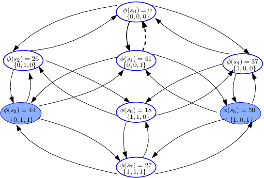
We compared the performance of sensor coverage game under LLL and ML based on CDA. We selected a small setup with three sensors in a grid of size to keep the system tractable. The sensor were located at . Each sensor had a fixed sensing range, which enabled us to represent the action set as on or off, i.e., for . Thus, the size of the state space was eight from to . The state corresponded to the joint action profile that is the binary equivalent of of . There are two equilibrium configurations and , where and . Moreover, is the potential maximizer. The results are presented in Fig. 5.
For three sensors, there were eight possible configurations, The utility of each configuration along with a state transition diagram is presented in 5(a), which is same for both the dynamics. The outputs of all the iterations of CDA for ML and LLL are presented in the figures ranging from 5(b)-5(f) and 5(g)-5(l) respectively. A simple comparison of the two sets of figures verified the analysis presented in the previous section. The cycles in the iterations for ML and for LLL were the same, as shown in figures 5(c)-5(f) and 5(i)-5(l) respectively. For each of these cycles, .
For the initial condition , the difference in the paths to stochastically stable states can also be observed from Figs. 5(b) and 5(g)-5(h). In the case of ML, the sensor configuration can reach either of the two equilibrium configurations through , resulting in the formation of the cycle . However, under LLL, the sensor configuration will first hit the potential maximizer through as shown by the cycle . In the next iteration, is added to the cycle instead of , which signifies that the network configuration will cycle between the states , , and exponentially many times before hitting for the first time.
IX Conclusions
We highlighted a critical issue with stochastic stability as a solution concept, which is its inability to distinguish between learning rules that lead to the same steady-state behavior. To address this problem, we presented a comprehensive framework for analyzing and comparing the transient performance of such learning dynamics. In the proposed framework, the main contribution was to identify cycle decomposition of Markov chains as a set of tools that enabled the comparative analysis of the stochastic learning dynamics. Moreover, we selected the expected hitting time to the set of Nash equilibria and the exit time from a subset of state space as important parameters to compare the performance of stochastic learning rules. We selected LLL and ML as representative members of the class of stochastic learning dynamics and showed that both of these dynamics have the same stochastically stable states, but significantly different short and medium run behavior. Based on the proposed comparative analysis framework, we identified critical factors, which effect the expected hitting time to the set of Nash equilibria for LLL and ML. We also proved that the exit time from a subset of state space will always be higher for LLL as compared to ML.
References
- [1] D. Foster and P. Young, “Stochastic evolutionary game dynamics∗,” Theoretical population biology, vol. 38, no. 2, pp. 219–232, 1990.
- [2] H. P. Young, “The evolution of conventions,” Econometrica, vol. 61, no. 1, pp. 57–84, January 1993.
- [3] M. Kandori, G. J. Mailath, and R. Rob, “Learning, mutation, and long run equilibria in games,” Econometrica: Journal of the Econometric Society, pp. 29–56, 1993.
- [4] L. E. Blume, “The statistical mechanics of strategic interaction,” Games and economic behavior, vol. 5, no. 3, pp. 387–424, 1993.
- [5] A. Montanari and A. Saberi, “Convergence to equilibrium in local interaction games,” in Foundations of Computer Science, 2009. FOCS’09. 50th Annual IEEE Symposium on. IEEE, 2009, pp. 303–312.
- [6] J. R. Marden and J. S. Shamma, “Game theory and distributed control,” Handbook of game theory, vol. 4, pp. 861–900, 2012.
- [7] V. Auletta, D. Ferraioli, F. Pasquale, and G. Persiano, “Metastability of logit dynamics for coordination games,” in Proceedings of the twenty-third annual ACM-SIAM symposium on Discrete Algorithms. SIAM, 2012, pp. 1006–1024.
- [8] V. Auletta, D. Ferraioli, F. Pasquale, P. Penna, and G. Persiano, “Convergence to equilibrium of logit dynamics for strategic games,” Algorithmica, vol. 76, no. 1, pp. 110–142, 2016.
- [9] G. E. Kreindler and H. P. Young, “Fast convergence in evolutionary equilibrium selection,” Games and Economic Behavior, vol. 80, pp. 39–67, 2013.
- [10] ——, “Rapid innovation diffusion in social networks,” Proceedings of the National Academy of Sciences, vol. 111, no. Supplement 3, pp. 10 881–10 888, 2014.
- [11] G. Ellison, D. Fudenberg, and L. A. Imhof, “Fast convergence in evolutionary models: A lyapunov approach,” Journal of Economic Theory, vol. 161, pp. 1–36, 2016.
- [12] D. Shah and J. Shin, “Dynamics in congestion games,” in ACM SIGMETRICS Performance Evaluation Review, vol. 38, no. 1. ACM, 2010, pp. 107–118.
- [13] I. Arieli and H. P. Young, Fast convergence in population games. Department of Economics, University of Oxford, 2011.
- [14] ——, “Stochastic learning dynamics and speed of convergence in population games,” Econometrica, vol. 84, no. 2, pp. 627–676, 2016.
- [15] G. Ellison, “Basins of attraction, long-run stochastic stability, and the speed of step-by-step evolution,” The Review of Economic Studies, vol. 67, no. 1, pp. 17–45, 2000.
- [16] D. K. Levine and S. Modica, “Dynamics in stochastic evolutionary models,” Theoretical Economics, vol. 11, no. 1, pp. 89–131, 2016.
- [17] M. I. Freidlin and A. D. Wentzell, “Random perturbations,” in Random Perturbations of Dynamical Systems. Springer, 1984, pp. 15–43.
- [18] E. Olivieri and E. Scoppola, “Markov chains with exponentially small transition probabilities: First exit problem from a general domain. I. The reversible case,” Journal of statistical physics, vol. 79, no. 3-4, pp. 613–647, 1995.
- [19] ——, “Markov chains with exponentially small transition probabilities: first exit problem from a general domain. II. The general case,” Journal of statistical physics, vol. 84, no. 5, pp. 987–1041, 1996.
- [20] O. Catoni, “Metropolis, simulated annealing, and iterated energy transformation algorithms: Theory and experiments,” Journal of Complexity, vol. 12, no. 4, pp. 595–623, 1996.
- [21] O. Catoni and R. Cerf, “The exit path of a markov chain with rare transitions,” ESAIM: Probability and Statistics, vol. 1, pp. 95–144, 1997.
- [22] A. Bovier and F. den Hollander, Metastability: a potential-theoretic approach. Springer, 2016, vol. 351.
- [23] M. Freidlin and L. Koralov, “Metastable distributions of markov chains with rare transitions,” Journal of Statistical Physics, pp. 1–21, 2017.
- [24] C. Daskalakis, P. W. Goldberg, and C. H. Papadimitriou, “The complexity of computing a nash equilibrium,” SIAM Journal on Computing, vol. 39, no. 1, pp. 195–259, 2009.
- [25] X. Chen, X. Deng, and S.-H. Teng, “Settling the complexity of computing two-player nash equilibria,” Journal of the ACM (JACM), vol. 56, no. 3, p. 14, 2009.
- [26] A. Trouve, “Cycle decompositions and simulated annealing,” SIAM Journal on Control and Optimization, vol. 34, no. 3, pp. 966–986, 1996.
- [27] H. Jaleel and J. S. Shamma, “Transient response analysis of metropolis learning in games,” IFAC-PapersOnLine, vol. 50, no. 1, pp. 9661–9667, 2017.
- [28] M. Mäs and H. H. Nax, “A behavioral study of “noise” in coordination games,” Journal of Economic Theory, vol. 162, pp. 195–208, 2016.
- [29] W. H. Sandholm, “Pairwise comparison dynamics and evolutionary foundations for nash equilibrium,” Games, vol. 1, no. 1, pp. 3–17, 2009.
- [30] J. R. Marden and J. S. Shamma, “Revisiting log-linear learning: Asynchrony, completeness and payoff-based implementation,” Games and Economic Behavior, vol. 75, no. 2, pp. 788–808, 2012.
- [31] J. R. Marden and A. Wierman, “Distributed welfare games,” Operations Research, vol. 61, no. 1, pp. 155–168, 2013.
- [32] O. Catoni, “Simulated annealing algorithms and markov chains with rare transitions,” in Séminaire de probabilités XXXIII. Springer, 1999, pp. 69–119.