Linear Mixed-Effects Models for Non-Gaussian Repeated Measurement Data

Laird and Ware (1982) were the first authors to consider modelling repeated measurements as noisy versions of underlying signals that can be decomposed into fixed effects, ${\boldsymbol{\mathrm{a}}}_{i}^{\top}{\boldsymbol{\mathrm{\alpha}}}+{\boldsymbol{\mathrm{x}}}_{ij}^{\top}{\boldsymbol{\mathrm{\beta}}}$, and random effects, ${\boldsymbol{\mathrm{d}}}_{ij}^{\top}{\boldsymbol{\mathrm{U}}}_{i}$, leading to the mixed-effects model

where $n_{i}$ is the number of measurements on the $i$th subject, $m$ is the number of subjects, the individual-level ${\boldsymbol{\mathrm{U}}}_{i}$ are mutually independent, zero-mean multivariate Normally distributed, ${\boldsymbol{\mathrm{U}}}_{i}\sim{\rm MVN}({\boldsymbol{\mathrm{0}}},{\boldsymbol{\mathrm{\Sigma}}})$, and the $Z_{ij}$ are mutually independent ${\rm N}(0,1)$.

A widely-used special case of (1) is the “random-intercept-and-slope” model in which each subject’s random effect is a linear function of time. This model is very useful when the data contain only a small number of repeated measurements per individual. With longer sequences, the assumption that individual random effect trajectories can be approximated by straight lines becomes implausible. Diggle (1988) proposed adding to the model a time-varying random-effect term, $W_{i}(t_{ij})$, specified as a stationary stochastic process. Taylor et al. (1994) and Diggle et al. (2015) later considered non-stationary options for $W_{i}(t_{ij})$. The general specification for models of this kind is that

where, in addition to the notation already introduced, the $W_{i}(t)$ are independent copies of a continuous-time Gaussian process with mean zero and covariance function $\gamma(t,t^{\prime})={\rm Cov}\{W_{i}(t),W_{i}(t^{\prime})\}$. We consider the elements of both the ${\boldsymbol{\mathrm{a}}}_{i}$ and the ${\boldsymbol{\mathrm{x}}}_{ij}$ to be pre-specified constants. This implicitly assumes, in particular, that if any time-varying covariate is not pre-specified, it is stochastically independent of all other terms in the model, hence conditioning on it is innocuous. We can then drop the term ${\boldsymbol{\mathrm{a}}}_{i}^{\top}\alpha$ in (2) by allowing elements of ${\boldsymbol{\mathrm{x}}}_{ij}$ to take identical values for all $j$ associated with any fixed $i$. For the covariance function $\gamma(t,t^{\prime})$, we use the stationary Matérn (1960) family,

where $\Gamma(\phi)$ is the complete gamma function, $\phi$ is a shape parameter, $\kappa$ is a scale parameter measured in units of time and $K_{\phi}$ is a modified Bessel function of order $\phi$. The corresponding Gaussian process $W_{i}(t)$ is $r$ times mean-square differentiable if $\phi>r$. An alternative way of capturing non-linear behaviour of repeated measurements is to specify the random effects as regression splines or polynomials with stochastic coefficients (Fitzmaurice et al., 2011, Chapter 19). We do not consider these approaches in this paper, since they appear to us less natural than the stochastic process approach based on (3) and would require many more parameters to achieve the same flexibility in shape.

Likelihood-based inference for the model (2) is straightforward. The likelihood function is a product of $m$ multivariate Normal densities with dimensions $n_{i}$. For typical study designs the $n_{i}$ are small enough that the required matrix calculations are not computationally demanding.

In the continuous-time setting, it is helpful to exploit an alternative representation of $W(\cdot)$ as the solution to a stochastic differential equation,

where ${\cal D}$ is a differential operator and $Z(t)$ is continuous-time white noise (Lindgren et al., 2011). For example, the integrated random walk model used by Diggle et al. (2015) corresponds to ${\cal D}=\frac{\partial^{2}}{\partial t^{2}}$, whilst the Matérn model corresponds to

In applications where only the regression parameters $\beta$ are of scientific interest, estimating equations offer an alternative to likelihood-based estimation. In the current context, this approach was introduced by Liang and Zeger (1986), working in the wider setting of generalised linear models. For linear models, the approach consists of estimating $\beta$ by weighted least squares, hence

where, for each $i$, ${\boldsymbol{\mathrm{Y}}}_{i}=(Y_{i1},\ldots,Y_{in_{i}})^{\top}$, ${\boldsymbol{\mathrm{x}}}_{i}$ is the $n_{i}$ by $k$ matrix whose $j$th row is ${\boldsymbol{\mathrm{x}}}_{ij}^{\top}$ and the ${\boldsymbol{\mathrm{F}}}_{i}$ are weight matrices. Re-writing (5) in an obvious shorthand notation as $\tilde{{\boldsymbol{\mathrm{\beta}}}}={\boldsymbol{\mathrm{D}}}{\boldsymbol{\mathrm{Y}}}$, inference for ${\boldsymbol{\mathrm{\beta}}}$ uses the result that $\tilde{\beta}$ is asymptotically multivariate Gaussian with mean ${\boldsymbol{\mathrm{\beta}}}$ and variance ${\boldsymbol{\mathrm{D}}}{\boldsymbol{\mathrm{C}}}{\boldsymbol{\mathrm{D}}}^{\top}$, where ${\boldsymbol{\mathrm{C}}}={\rm Var}({\boldsymbol{\mathrm{Y}}})$, a block-diagonal matrix with non-zero blocks, ${\boldsymbol{\mathrm{C}}}_{i}={\rm Var}({\boldsymbol{\mathrm{Y}}}_{i})$. If ${\boldsymbol{\mathrm{F}}}_{i}={\boldsymbol{\mathrm{C}}}_{i}^{-1}$, then $\tilde{{\boldsymbol{\mathrm{\beta}}}}$ is the maximum likelihood (ML) estimator for ${\boldsymbol{\mathrm{\beta}}}$.

The basic idea behind (5) is to choose, rather than estimate, a set of matrices ${\boldsymbol{\mathrm{F}}}_{i}$ that reflect a reasonable working covariance structure for the matrices ${\boldsymbol{\mathrm{C}}}_{i}={\rm Var}({\boldsymbol{\mathrm{Y}}}_{i})$, but not to rely on the correctness of the chosen structure. Instead, the unknown matrix ${\boldsymbol{\mathrm{C}}}_{i}$ is replaced by a non-parametric estimate, $\tilde{{\boldsymbol{\mathrm{C}}}}_{i}$. One such set of estimates is given by $\tilde{{\boldsymbol{\mathrm{C}}}}_{i}=n_{i}^{-1}({\boldsymbol{\mathrm{Y}}}_{i}-{\boldsymbol{\mathrm{x}}}_{i}\tilde{{\boldsymbol{\mathrm{\beta}}}})({\boldsymbol{\mathrm{Y}}}_{i}-{\boldsymbol{\mathrm{x}}}_{i}\tilde{{\boldsymbol{\mathrm{\beta}}}})^{\top}.$ Individually, each $\tilde{{\boldsymbol{\mathrm{C}}}}_{i}$ is a very poor estimate of ${\boldsymbol{\mathrm{C}}}_{i}$, but the implicit averaging in (5) leads to consistent estimation of ${\rm Var}(\tilde{{\boldsymbol{\mathrm{\beta}}}})$ in the limit $m\rightarrow\infty$ for fixed $n_{i}$.

The existing literature on non-Gaussian models takes as its starting point a linear model with correlated errors,

where, in the case of a common set of follow-up times $t_{1},...,t_{n}$ for each subject, the ${\boldsymbol{\mathrm{S}}}_{i}=(S_{i1},\ldots,S_{in})^{T}$ are independent copies of a zero-mean multivariate Normal random vector (Jennrich and Schluchter, 1986). Most authors only consider the Laird-Ware approach as presented in (1), where

Liu and Rubin (1995), Lange et al. (1989) and Pinheiro et al. (2001) replaced each $S_{ij}$ in (6) or (7) by $S^{*}_{ij}=S_{ij}/\sqrt{V_{i}}$ where the $V_{i}$ are mutually independent unit-mean gamma-distributed random variables. They estimated the model parameters by maximum likelihood using an EM algorithm (Dempster et al., 1977). Lin and Wang (2011) considered Bayesian methods of inference for the same class of models. Matos et al. (2013) extended the work of Pinheiro et al. (2001) to allow censored outcomes.

Song et al. (2007) and Zhang et al. (2009) considered an extension to Lange et al. (1989) by allowing the gamma-distributed scaling factor $V_{i}$ to apply to either one of the two components on the right hand side of (7). Lin and Lee (2007) apply the gamma-distributed scaling factor only to the random effect term ${\boldsymbol{\mathrm{d}}}_{ij}^{\top}{\boldsymbol{\mathrm{U}}}_{i}$, but also replace the mutually independent $Z_{ij}$ by a set of autoregressive processes; this restricts its applicability to data with equally-spaced measurement times.

Rosa et al. (2003) and Tian et al. (2008) also used the formulation $S^{*}_{ij}=S_{ij}/\sqrt{V_{i}}$ but without restricting the $V_{i}$ to be gamma-distributed. Lange and Sinsheimer (1995) called the resulting family of distributions the Normal/independent family. The R package heavy (Osorio, 2016) fits this class of models. In a series of papers, V.H. Lachos and colleagues have developed methodology for fitting non-linear mixed models using the Normal/independent family; see Lachos et al. (2009), Lachos et al. (2010), Zeller et al. (2010), Lachos, Bandyopadhyay and Dey (2011), Cabral et al. (2012), Lachos et al. (2012) and Lachos et al. (2013), also independent contributions by Verbeke and Lesaffre (1996), Sun et al. (2008), Ho and Lin (2010), De la Cruz (2014), Zhang et al. (2015) and Yavuz and Arslan (2016).

Several authors have extended the single-term modelling framework (7) by de-coupling the scalings of the random effect term and the measurement error term. See, for example, Rosa et al. (2004), Aralleno-Valle et al. (2007), Jara et al. (2008), Meza et al. (2012), Choudhary et al. (2014) and Bai et al. (2016). Lu and Zhang (2014) extended the approach to include consideration of non-ignorable drop-out.

Wang and Fan (2011), Wang and Fan (2012), Lin and Wang (2013) and Kazemi et al. (2013) used the Normal/independent family to model multivariate repeated measurement data.

Other authors have taken a semi-parametric approach to the problem, for example by using a Dirichlet process prior for the random effects. See Kleinman and Ibrahim (1998), Ghidey et al. (2004), Tao et al. (2004), Subtil and Rabilloud (2010), Davidian and Gallant (1993), Zhang and Davidian (2001) and Vock et al. (2012). Koller (2016) has considered robust estimating equations.

We have found only two papers that apply the single-term formulation (7) to the general form of the model (2) with three stochastic components (Stirrup et al, 2015; Asar et al, 2016), and none that allow the three scaling factors to be de-coupled.

A flexible choice for the noise term in (8) is the multivariate generalised hyperbolic (GH) distribution (Barndorff-Nielsen, 1977; Vilca, Balakrishnan and Zeller, 2014). This distribution can be generated from the mixture representation (9) by specifying a generalised inverse Gaussian distribution (GIG) for $V$. The density function of the GIG distribution is

where $K_{p}$ is the modified Bessel function of the third kind, of order $p$, and $a$ and $b$ are positive-valued parameters. We denote this distribution by ${\rm GIG}(p,a,b)$ and refer the reader to Jørgensen (1982) for more details. An important property of this distribution is that for any $c>0$, $cV\sim{\rm GIG}(p,a/c,cb)$. Another property that is useful for the construction of the sampling-based inferential algorithms that we introduce in Sections 4.2 and 4.3 is that the conditional distribution of $V$ given the observed data is also GIG.

The GH distribution includes several widely-used distributions as special cases, for example the Student’s $t$, generalized asymmetric Laplace (GAL), Normal-inverse Gaussian (NIG) and Cauchy (CH) distributions. Specific parameter configurations for the distributions of $V$ that give each of these special cases are presented in Table 1.

Since the measurement noise is univariate, we can write the mixture representation (9) as

where $Z_{ij}^{*}\sim{\rm N}(0,1)$. To maintain the interpretation of $\sigma^{2}$ as the variance of the noise, we constrain the values of the GIG parameters $a$, $b$ and $p$, so that ${\rm E}[V_{ij}]=1$ if ${\rm E}[V_{ij}]$ exists, and the mode of the distribution is one otherwise. We further set $\delta=\mu=0$ to ensure that the measurement noise is symmetric with ${\rm E}[Z_{ij}]=0$.

An alternative to (11) is to attach a single random variable $V_{i}$ to all of the noise terms $Z_{ij}$ on the $i$th subject, i.e. $Z_{ij}=\delta+\mu V_{i}+\sqrt{V_{i}}\sigma Z_{ij}^{*}$. The distribution of $V_{i}$ can then be interpreted as a random effect distribution for patient-specific measurement noise variance. Note, in particular, that this introduces stochastic dependence between $Z_{ij}$ and $Z_{ij^{\prime}}$ for $j\neq j^{\prime}$.

For the random effects, we let ${\boldsymbol{\mathrm{U}}}_{i}={\boldsymbol{\mathrm{\delta}}}+{\boldsymbol{\mathrm{\mu}}}V_{i}+\sqrt{V_{i}}\Sigma^{1/2}{\boldsymbol{\mathrm{U}}}_{i}^{*}$, where $V_{i}$ is a unit-mean GIG random variable and ${\boldsymbol{\mathrm{U}}}_{i}^{*}\sim{\rm MVN}({\boldsymbol{\mathrm{0}}},{\boldsymbol{\mathrm{I}}})$ with ${\boldsymbol{\mathrm{I}}}$ the identity matrix. To allow skewness in the distribution of the random effects we do not require that ${\boldsymbol{\mathrm{\mu}}}={\boldsymbol{\mathrm{0}}}$, but we then ensure that ${\rm E}[{\boldsymbol{\mathrm{U}}}_{i}]={\boldsymbol{\mathrm{0}}}$ by setting ${\boldsymbol{\mathrm{\delta}}}=-{\boldsymbol{\mathrm{\mu}}}$.

The simplest way to introduce a non-Gaussian stochastic process term in (8) would again be to include a subject-specific scaling, i.e. $W_{i}(t)=V_{i}W_{i}^{*}(t)$, where $V_{i}$ again follows a unit-mean GIG distribution. However, this approach would not be able to capture interesting within-subject departures from Gaussian behaviour, e.g. jumps or asymmetries in the sample paths of $W_{i}(t)$. To provide the required flexibility, we instead use non-Gaussian generalisations of the stochastic differential equation (4). Specifically, we propose modelling the $W_{i}(t)$ as independent copies of the solution to

where the $L_{i}$ are independent copies of a non-Gaussian Lévy process, i.e. a process with independent and stationary increments. In practice, we work with a discretised version of (12), for which Bolin (2014) showed that a type-G Lévy process for $L_{i}(t)$ is a suitable candidate. The implication is that the increments of $L_{i}$ have a distribution that corresponds to the specification given by (9).

One approach would therefore be to choose the distribution of $V$ in (9) as a GIG distribution, which would yield the Hyperbolic processes of Eberlein (2001). However, as noted earlier, we require the distribution of $V$ to be closed under convolution (Wallin and Bolin, 2015). Also, the stochastic gradient methods for parameter estimation to be introduced in Section 4 require sampling from the conditional distribution of $V$ given all other components in the model. Within the GH family, the NIG, GAL, and Cauchy distributions are the only ones that meet these requirements (Podgórski and Wallin, 2016). Using any of these distributions for the increments of $L_{i}$ in (12) results in models with the same covariance structure as if $L_{i}$ were Gaussian, but with more general marginal distributions. The NIG choice makes $L_{i}$ a NIG process (Barndorff-Nielsen, 1997a), which has been used in financial modeling; see Barndorff-Nielsen (1997b), Bibby and Sørensen (2003), Tankov (2003) and Eberlein (2001). We will focus on the NIG case in order to keep the presentation brief, but the modifications needed to cover the GAL and Cauchy counterparts are straightforward.

For computational purposes, we use a discretised version of the stochastic differential equation (12) as follows; see also Lindgren and Rue (2008). Firstly, denote by $\left\langle{f},\,{g}\right\rangle$ the standard inner product on $\R$, $\left\langle{f},\,{g}\right\rangle=\int f(t)g(t)dt$. We restrict $W(t)$ to a finite interval, $0\leq t\leq t_{0}$, and impose Neumann boundary conditions, $dW(0)=dW(t_{0})=0$. The so-called weak form of (12) is a function of $W(t)$ that satisfies the equation,

for a specified set of test functions $\psi(t)$. We now use the following low-rank approximation,

where ${\boldsymbol{\mathrm{W}}}=(W_{1},\ldots,W_{K})$ is a vector of random variables and the $\phi_{k}(t)$ are basis functions. We use a set of piecewise linear basis functions such that

and, for $k=2,3,...,(K-1)$,

where $0=s_{1}<s_{2}<\ldots<s_{K-1}<s_{K}=t_{0}$.

We use the Galerkin finite element method to compute the stochastic weights, $W_{k}$. This consists of setting all the test functions to the basis functions, i.e. $\psi_{k}=\phi_{k}$ for all $k$, and computing the $W_{k}$ by solving the system of equations defined by equation (13), i.e.

where $L_{k}=\left\langle{\phi_{k}},\,{dL}\right\rangle$, and $K_{kk^{\prime}}=\left\langle{\phi_{k}},\,{\mathcal{D}\phi_{k^{\prime}}}\right\rangle$ is a discretised version of the differential operator $\mathcal{D}$. For the NIG version of the model, we approximate the distribution of $L_{k}$ by

where $Z_{k}\sim{\rm N}(0,1)$, $h_{k}=\left\langle{\phi_{k}},\,{1}\right\rangle$, and $V_{k}\sim{\rm IG}(\nu,h_{k}^{2}\nu)$ (Bolin, 2014). It follows that the distribution for the stochastic weight-vector ${\boldsymbol{\mathrm{W}}}$ conditional on $V$ can be written as

Since the parameter $\nu$ determines the value of $b$ in the NIG distribution, it controls the tails of the marginal distribution of the process. The limit when $\nu\rightarrow 0$ is the Cauchy process, whereas the limiting case $\nu\rightarrow\infty$ is a Gaussian process. These are exactly the properties we need in order to use our likelihood-based methods to assess whether a standard, and undeniably convenient, Gaussian assumption for any or all of the stochastic components of (8) is adequate.

The full GH family of distributions is difficult to fit to data, because the full log likelihood surface is largely flat, which makes the model parameters almost non-identifiable. The problem persists for some of the sub-families discussed above. For example, a NIG distribution converges to a Cauchy distribution as $a\rightarrow 0$ and to a Gaussian distribution as $a\rightarrow\infty$ and $b\rightarrow\infty$ at the same rate. Recognising these limiting cases is important in practice, since typically the densities are numerically unstable at the edges of the parameter space. Moreover, handling the NIG distribution is computationally more demanding than the Gaussian distribution. Rules for switching between the distributions, or equivalently setting finite boundaries to the parameter space, require some guidance. This can be achieved by the total variation (TV) distance between pairs of densities. For illustration, we consider the TV distance between two symmetric, zero-mean distributions. For instance, to compare the NIG distribution for fixed $a$ with the Cauchy distribution, we calculate

To simplify the calculations needed to find the Cauchy distribution ${\rm CH}(0,0,b_{CH})$ that is closest to the ${\rm NIG}(0,0,a,b_{NIG})$ distribution we use the proposition below, which shows that it suffices first to find the Cauchy distribution closest to ${\rm NIG}(0,0,a,1)$, then rescale the shape parameter by $b_{NIG}$.

The proposition can also be used to compare NIG and Gaussian distributions. Figure 2 shows the TV distances between the NIG and Cauchy, and between the NIG and Gaussian, as functions of $a$. For $a=0.001$, the TV distance between the NIG and Cauchy is less than that between two Bernoulli distributions whose probabilities differ by $0.002$. The same applies to the TV distance between the NIG and Normal when $a=250$. This suggests that setting the boundary of $a$ at these values, i.e., switching from the NIG to the Gaussian when $a>250$ and to the Cauchy when $a<0.001$, is a conservative strategy for parameter estimation, or for prediction within or close to the observed range of the data. Since the differences between the distributions are in their tails, prediction of extreme events could be affected by the switching even when one cannot tell empirically which density should be used. For example, the NIG distribution has exponential tails for all values $a$, whereas the Cauchy has polynomial tails.

Our specification of a Normal-variance mixture for each of the stochastic components of (8) makes likelihood-based inference practicable via the following hierarchical representation of the model. For subject $i$, let ${\boldsymbol{\mathrm{V}}}_{i}^{Z}$, $V_{i}^{U}$, and ${\boldsymbol{\mathrm{V}}}_{i}^{W}$ denote the stochastic variance factors corresponding to the noise, random effect and stochastic process components of (8), and write ${\boldsymbol{\mathrm{Y}}}_{i}=(Y_{i1},\ldots,Y_{in_{i}})^{\top}$ for the corresponding set of repeated measurements. Let $W_{i}=\{W_{ik}:k=1,\ldots,K\}$ be the stochastic weight vector for the $i$th subject in the approximation of $W_{i}(t)$ given by (14), and ${\boldsymbol{\mathrm{A}}}_{i}$ the $n_{i}$ by $K$ matrix with $(j,k)$th element $\phi_{k}(t_{ij})$. Write ${\boldsymbol{\mathrm{x}}}_{i}$ and ${\boldsymbol{\mathrm{d}}}_{i}$ for the matrices with $j$th row ${\boldsymbol{\mathrm{x}}}_{ij}^{\top}$ and ${\boldsymbol{\mathrm{d}}}_{ij}^{\top}$, respectively. Finally, let ${\boldsymbol{\mathrm{\Theta}}}$ denote the complete set of model parameters. The model for the $i$th subject then has the following hierarchical representation

These collectively determine the contribution of the $i$th subject to the log-likelihood, $L({\boldsymbol{\mathrm{\Theta}}};{\boldsymbol{\mathrm{y}}}_{i})$. As the vectors ${\boldsymbol{\mathrm{Y}}}_{i}$ from the $m$ subjects are independent, the overall log-likelihood is

The computations required for maximum likelihood estimation are cumbersome for problems that involve longitudinal data-sets with large numbers of subjects and repeats, even using the computationally efficient approximation (14). Our proposed algorithm for ML estimation therefore uses a stochastic gradient method that calculates the gradient of the objective function at each step of the maximisation by sub-sampling.

A stochastic gradient method for the general problem of minimising an objective function $f({\boldsymbol{\mathrm{\Theta}}})$ starts with an initial guess ${\boldsymbol{\mathrm{\Theta}}}^{(0)}$, and then iteratively updates ${\boldsymbol{\mathrm{\Theta}}}$ according to

where $Q_{n}({\boldsymbol{\mathrm{\Theta}}})$ is a random variable such that ${\rm E}[Q_{n}({\boldsymbol{\mathrm{\Theta}}})]=\nabla f({\boldsymbol{\mathrm{\Theta}}})$ and $\alpha_{i}$ is a sequence of positive numbers such that $\sum_{n=1}^{\infty}\alpha_{n}=\infty$ and $\sum_{n=1}^{\infty}\alpha_{n}^{2}<\infty$. Under mild regularity conditions, the resulting sequence ${\boldsymbol{\mathrm{\Theta}}}^{(n)}$ converges to a stationary point of $f({\boldsymbol{\mathrm{\Theta}}})$ (Kushner and Yin, 2003; Andrieu et al., 2007).

For maximum likelihood estimation, $f({\boldsymbol{\mathrm{\Theta}}})=-L({\boldsymbol{\mathrm{\Theta}}};{\boldsymbol{\mathrm{y}}})$. If the data-set contains a large number of subjects we use only a small, randomly sampled subset in each iteration to generate an efficient stochastic gradient method. For this purpose, $\nabla L({\boldsymbol{\mathrm{\Theta}}};{\boldsymbol{\mathrm{y}}})$ can be replaced by the random variable

where the $J_{i}$ are independent Bernoulli random variables with ${\rm P}(J_{i}=1)=1/s$. Since ${\rm E}[\nabla L_{s}({\boldsymbol{\mathrm{\Theta}}};{\boldsymbol{\mathrm{y}}})]=\nabla L({\boldsymbol{\mathrm{\Theta}}};{\boldsymbol{\mathrm{y}}})$ for any $s$, the resulting stochastic gradient method (15) will converge to a stationary point of the log-likelihood. Our experience, for example with the two case-studies that we describe in Section 5, has been that for data-sets containing a large number of subjects, often we need TO access only a small proportion of the available measurement sequences ${\boldsymbol{\mathrm{Y}}}_{i}$ at each iteration in order to estimate the parameters reliably. Our proposed algorithm therefore becomes

where the multiplier $\alpha_{n}/m$ highlights that for numerical stability the step length should scale with the number of subjects in the complete data-set.

For our non-Gaussian models, an additional complication is that the likelihood is not available in an explicit form. However, using Fisher’s identity (Dempster et al., 1977) we can compute the gradient of the log-likelihood without computing the log-likelihood itself. For all versions of our model, the log-likelihood conditional on the variance components, ${\boldsymbol{\mathrm{V}}}=\{{\boldsymbol{\mathrm{V}}}_{i}^{W},{\boldsymbol{\mathrm{V}}}_{i}^{U},{\boldsymbol{\mathrm{V}}}_{i}^{Z}\}_{i=1}^{m}$, is Gaussian and thus explicit. Fisher’s identity then gives

where $L_{s}({\boldsymbol{\mathrm{\Theta}}};{\boldsymbol{\mathrm{y}}})$ is the augmented likelihood and is explicitly available, since ${\boldsymbol{\mathrm{Y}}},{\boldsymbol{\mathrm{V}}}|{\boldsymbol{\mathrm{\Theta}}}$ is Gaussian and $V|{\boldsymbol{\mathrm{\Theta}}}$ is GIG.

The expectation is not, in general, explicit but can be approximated by Monte Carlo sampling from the conditional distribution ${\boldsymbol{\mathrm{V}}}|{\boldsymbol{\mathrm{y}}};{\boldsymbol{\mathrm{\Theta}}}$. We use a Gibbs sampler and iterate between sampling from the conditional distributions ${\boldsymbol{\mathrm{V}}}|{\boldsymbol{\mathrm{X}}},{\boldsymbol{\mathrm{Y}}};{\boldsymbol{\mathrm{\Theta}}}$ and ${\boldsymbol{\mathrm{X}}}|{\boldsymbol{\mathrm{V}}},{\boldsymbol{\mathrm{Y}}};{\boldsymbol{\mathrm{\Theta}}}$, where ${\boldsymbol{\mathrm{X}}}$ denotes all the conditional Gaussian components, i.e. ${\boldsymbol{\mathrm{X}}}=\{{\boldsymbol{\mathrm{U}}}_{i},{\boldsymbol{\mathrm{W}}}_{i}\}_{i=1}^{m}$. Convergence of algorithms of this kind is studied in Andrieu et al. (2007).

When using stochastic gradient optimization to maximise over many parameters, it is important to scale the gradient by a pre-conditioner to give a Newton-like iteration:

One option for the pre-conditioner is

Calculation of ${\boldsymbol{\mathrm{I}}}^{*}({\boldsymbol{\mathrm{\Theta}}})$ is typically easy, since $\nabla\nabla L_{s}({\boldsymbol{\mathrm{\Theta}}};{\boldsymbol{\mathrm{y}}},{\boldsymbol{\mathrm{y}}})$ is often explicit and can be calculated at the same time as the gradient. Lange and Sinsheimer (1995) describe the connection between (18) and the EM algorithm. However, if the same variables are used for the Monte Carlo estimates of the expectations in ${\boldsymbol{\mathrm{I}}}_{.}({\boldsymbol{\mathrm{\Theta}}})$ and $Q_{i}({\boldsymbol{\mathrm{\Theta}}})$, the joint updating step (17) will be biased due to correlation between the two estimated quantities. A pre-conditioner that is less problematic numerically, and is often explicitly available, is the complete Fisher Information (cFIM),

Note that in (19), the expectation is taken over both ${\boldsymbol{\mathrm{Y}}}$ and ${\boldsymbol{\mathrm{V}}}$. The standard Fisher information matrix,

is seldom explicit and thus cannot be used as a pre-conditioner. However, we do need to estimate either the standard or the observed Fisher information matrix,

in order to calculate confidence intervals for the estimated parameters. We estimate ${\boldsymbol{\mathrm{I}}}_{oFIM}({\boldsymbol{\mathrm{\Theta}}})$ using Louis’s identity (Louis, 1982),

Both terms on the right-hand side of (20) can be estimated by Monte Carlo sampling, as proposed for $\nabla L_{s}({\boldsymbol{\mathrm{\Theta}}};{\boldsymbol{\mathrm{y}}})$ in (16).

We could estimate ${\boldsymbol{\mathrm{I}}}_{FIM}({\boldsymbol{\mathrm{\Theta}}})$ by an additional sampling step, using the fact that ${\boldsymbol{\mathrm{I}}}_{FIM}({\boldsymbol{\mathrm{\Theta}}})={\rm E}_{{\boldsymbol{\mathrm{Y}}}}[{\boldsymbol{\mathrm{I}}}_{oFIM}({\boldsymbol{\mathrm{\Theta}}})|{\boldsymbol{\mathrm{\Theta}}}]$.

An issue with the sub-sampling method described in (4.2) is that the sub-sampled matrices of covariates, ${\boldsymbol{\mathrm{x}}}_{i}$, may not be of full rank. If this is the case, none of the pre-conditioners above can be used. On the other hand, regular sub-sampling without any pre-conditioners may result in large Monte Carlo variation in the estimated gradient. The cystic fibrosis case-study that we shall describe in Section 5.1 provides an example, where the data are stratified into birth cohorts whose effects are important, but one of the cohorts contains only seven patients. This issue is related to sub-sampling for S-estimation algorithms in linear regression models (Koller and Stahel, 2016). Nonetheless, we could not find a satisfactory solution in the literature that could be applied in the current context. To address the issue, we therefore introduce the following sub-sampling procedure, which we call the grouped sub-sampler. The procedure first builds $k+1$ groups of subjects, $\mathcal{G}_{0},\mathcal{G}_{1},\ldots,\mathcal{G}_{k}$, in such a way that the matrices $\sum_{i\in\mathcal{G}_{k}}{\boldsymbol{\mathrm{x}}}_{i}$ have full column ranks for $k\geq 1$. The procedure for forming the groups is described in the pseudo-code in Algorithm 1. Let $m_{g}$ be the number of subjects in group $g$, and write $\bar{m}=k^{-1}\sum_{g=1}^{k}m_{g}$. A sub-sampling step selects approximately $M$ subjects by first selecting all subjects in $r<k$ groups chosen at random from $\mathcal{G}_{1},\ldots,\mathcal{G}_{k}$, then adding $M-\bar{m}\times m_{g}$ subjects chosen at random from $\mathcal{G}_{0}$. The expected number of sub-sampled subjects is then $M$, and the matrix of covariates for the sub-sampled subjects has full column rank. To obtain an unbiased estimate of the gradient, we then assign weights $k/m_{g}$ to the subjects sampled from the groups $\mathcal{G}_{1},\ldots,\mathcal{G}_{k}$, and weight $m_{0}/(M-\bar{m}\times m_{g})$ to those sampled from $\mathcal{G}_{0}$.

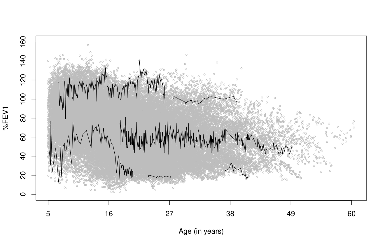
Our first application uses data on the lung function of cystic fibrosis patients, taken from the Danish Cystic Fibrosis register. The patients are all aged over 5 years, and entered the database between 1969 and 2010. The outcome variable is %FEV1 (per cent predicted forced expiratory volume in 1 second), a measure of lung function that is widely used as a descriptor of disease severity (Davies and Alton, 2009). The data, previously analysed by Taylor-Robinson et al. (2012), contain 70,448 measurements of %FEV1 on 479 patients with follow-up times approximately one month apart. For the analysis reported here, three patients who provided only one %FEV1 measurement have been excluded. Hence, 476 patients are available for the current analysis. Available covariates are: sex, age, birth cohort (decadal), presence/absence of pancreatic sufficiency, presence/absence of diabetes mellitus, and years after pseudomonas infection. The number of repeated measures per patient ranges between 2 and 597 with a median of 101.5. Total follow-up times ranged between 0.1 and 31.5 years with a median of 10.5. Of the 476 patients, 233 (48.9%) are female, 20 (4.2%) have pancreatic sufficiency, 14 (2.9%) have diabetes. Baseline ages range between 5.0 and 48.1 years with a median of 7.0. Cohort numbers are 7 (1.5%), 42 (8.8%), 109 (22.9%), 105 (22.1%), 141 (29.6%) and 72 (15.1%) for birth cohorts of 1948–1957, 1958–1967, $\ldots$, 1998–2007, respectively. Baseline %FEV1 values range between 10.4 and 140.3 with a mean of 78.5. Figure 3 shows traces for six patients, chosen to illustrate a range of total follow-up times and patterns of the outcome variable, %FEV1.

Fitting a model to these data serves two purposes. The first is to characterise the mean response profile of lung function in cystic fibrosis patients, adjusted for relevant covariates. The second is to quantify the extent to which a subject’s early results are predictive of their long-term prognosis.

We let $Y=$ %FEV1 and specify mixed effects models that fall within the general framework of (8). Specifically we consider

where the $W_{i}(t)$’s are mutually independent, continuous-time stochastic processes. We model this process as the solution to the stochastic differential equation $\left(\kappa^{2}-\frac{d^{2}}{dt^{2}}\right)^{1/2}W_{i}(t)=dL_{i}(t)$, which implies that $W_{i}(t)$ has an exponential covariance function, as in Taylor-Robinson et al. (2012).

In this example cohort effects are substantial, reflecting general improvements in the treatments available to CF patients over the time-period concerned. This, coupled with the small numbers of patients in some cohorts (e.g. 7 patients in 1948–1957), explains why the grouped sub-sampler described in Section 4.3 is needed.

To illustrate the effect of the sub-sampling, we first fit a Gaussian model, i.e assuming Gaussian distributions for $U_{i}$, $W_{i}(t)$ and $Z_{ij}$, with and without sub-sampling. In the former case, we sub-sample 20% of the patients, i.e. 96 out of 476. The resulting parameter tracks of the optimiser can be seen in Figure 4. In this example, there are $k=7$ sub-sampling groups, with an average group size of $8$ subjects, and two groups were sampled at each iteration. The running time for the $20,000$ iterations scales linearly with $M$, the number of patients sub-sampled at each iteration. In this example, sub-sampling reduced computing time by a factor of almost five. The variances of the sub-sampled estimates are relatively higher, but the final parameter estimates are almost identical.

To assess the suitability of the Gaussian distributional assumption we inspected quantile-quantile (QQ) plots of the standardised marginal residuals, $Y_{ij}-{\boldsymbol{\mathrm{x}}}_{ij}^{\top}{\boldsymbol{\mathrm{\beta}}}$ . The plot (not shown here) suggests some departure from the Gaussian, but as each marginal residual is composed of $U_{i}$, $W_{i}(\cdot)$ and $Z_{ij}$, the QQ plot is not able to detect the source of the departure. We therefore fit the model with a NIG assumption for each of the $U_{i}$, $W_{i}(\cdot)$ and $Z_{ij}$ components. The respective estimates of $\nu$ are 83.77, 0.34 and 0.48, which indicate the extent to which each component appears to exhibit non-Gaussian behaviour. The estimates of the fixed effect parameters, ${\boldsymbol{\mathrm{\beta}}}$, for Normal and NIG models are shown in Table 2. Standard error estimates, obtained using standard Fisher matrix, are generally lower under NIG than under Gaussian distributional assumptions. With regard to the statistical significance or otherwise of the estimates, we report two p-values, p-lower and p-upper, by taking into account Monte Carlo error in the parameter and standard error estimates. Lower and upper p-values indicate the same judgement on significance, except for pancreatic sufficiency under NIG. Note that this variable is highly unbalanced, with only 20 positives out of 476. Consequently, Normal and NIG models agree on the significance of the estimates, except for the interaction of age and cohort 1958.

Our second application uses clinical data on the kidney function of primary care patients from the northern English city of Salford who are in high-risk groups for chronic kidney disease. The outcome variable is eGFR (estimated Gromerular Filtration Rate, in mL/min per 1.73$\mbox{m}^{2}$ of body surface area), a proxy measurement for the patient’s renal function calculated as

where SCr stands for serum creatinine measured in $\mu$mol/L (Levey et al, 1999).

The data, previously analysed by Diggle et al. (2015), contain a total of 392,870 measurements on 22,910 patients, for whom total follow-up time ranged from zero (i.e. only baseline data is available) to 10.0 years, whilst the number of measurements of eGFR ranged from 1 to 305. Amongst the 22,910 patients, 11,833 (51.7%) were male. Baseline ages ranged between 13.7 and 102.1 with a mean of 65.4.

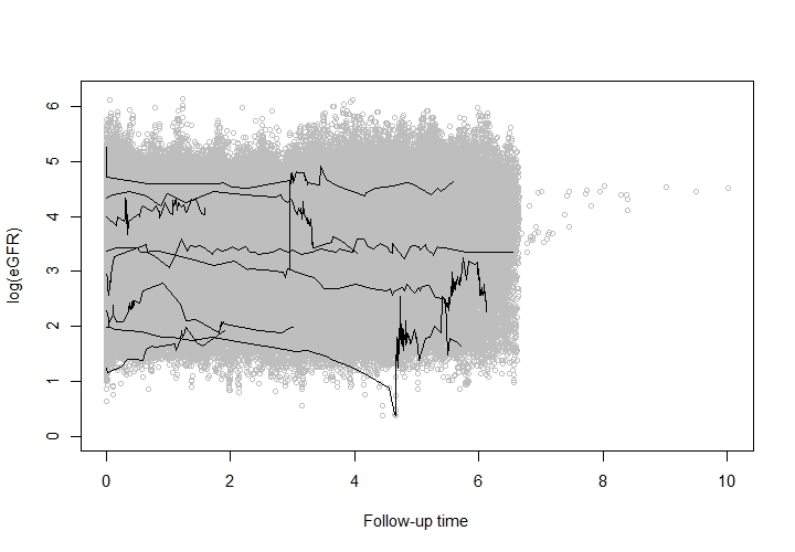
Figure 5 shows traces for eight patients, chosen to illustrate some particularly challenging features of the data. The unusually high degree of irregularity in the follow-up times reflects the fact that the data derive from routine clinical practice. In particular, some patients provided many repeated measurements over a relatively short time-period, probably during episodes of inter-current illness.

Clinical care guidelines in the UK include a recommendation that any person in primary care who appears to be losing kidney function at a relative rate of at least 5% per year should be considered for referral to specialist secondary care. Our primary objective in analysing these data is therefore to develop a method for identifying, for each subject and in real-time, when this criterion is first met.

As in Diggle et al. (2015), we use a log-transformed outcome variable, $Y=\log(\mbox{eGFR})$, and specify a model of the form

In (23), each ${\boldsymbol{\mathrm{x}}}_{ij}$ includes sex, baseline age, follow-up time ($t_{ij}$) and a piece-wise linear function of age with a slope change at age 56.5. The processes $W_{i}(t)$ are integrated random walks as in Diggle et al. (2015).

We first fit the model under Gaussian assumptions for the $U_{i}$, $W_{i}(\cdot)$ and $Z_{ij}$ components. The residual QQ plot shown as Figure 5 of Diggle et al. (2015) shows longer-than-Gaussian tails. As for the CF example, the source of this deviation from the Gaussian assumptions is unknown. Therefore, we proceed by assuming NIG distributions for each of the three stochastic components. Estimates of $\nu$ based on this model are 99.93, 0.01 and 0.19 for $U_{i}$, $W_{i}(\cdot)$ and $Z_{ij}$, respectively. As the magnitude of $\hat{\nu}$ for $U_{i}$ indicates close-to-Gaussian behaviour our final model assumes a Normal distribution for $U_{i}$, and NIG distributions for $W_{i}(\cdot)$ and $Z_{ij}$.

Figure 6 shows, for two patients, their observed data and the concurrent (“nowcasting”) probabilities of meeting the clinical guideline for referral to specialist care. These are derived from the predictive distributions $[Y_{ik}^{*}|Y_{i1},\ldots,Y_{ik}]$, where $Y_{ik}^{*}=Y_{ik}-Z_{ij}$; see (23). Results are shown for our preferred model, with Normally distributed $U_{i}$, and NIG distributed $W_{i}(\cdot)$ and $Z_{ij}$ components, and for the corresponding Gaussian model. As would be expected, for each patient the general pattern of the predictive probabilities is similar under both modelling assumptions, but there are some substantial quantitative differences and the ranking of each pair of predictive probabilities is not consistent. The two sets of model-based predictions reflect different partitionings of the intra-patient variation into signal and noise components, and the balance between the two is affected in subtle ways by the pattern of follow-up times and their associated measurements.

References

- Andrieu et al. (2007) Andrieu C., Moulines É. and Priouret P. (2007). Stability of stochastic approximation under verifiable conditions. SIAM Journal on Control and Optimization, 44, 283–312.
- Aralleno-Valle et al. (2007) Aralleno-Valle R. B., Bolfarine H. and Lachos V. H. (2007). Bayesian inference for skew-Normal linear mixed models. Journal of Applied Statistics 34, 663–682.
- Asar et al. (2016) Asar Ö., Ritchie JP, Kalra PA and Diggle PJ (2016). Short-term and long-term effects of acute kidney injury in chronic kidney disease patients: A longitudinal analysis. Biometrical Journal, 58(6), 1552–1566.
- Bai et al. (2016) Bai X., Chen K. and Yao W. (2016). Mixture of linear mixed models using multivariate distribution. Journal of Statistical Computation and Simulation 86, 771–787.
- Barndorff-Nielsen (1977) Barndorff-Nielsen O.E. 1977. Exponentially decreasing distributions for the logarithm of the particle size. Proceedings of the Royal Society London Series A. Mathematical and Physical Sciences, 353, 401–419.
- Barndorff-Nielsen (1997a) Barndorff-Nielsen, O. (1997a), Processes of normal inverse Gaussian type. Finance and Stochastics, 2, 41–68
- Barndorff-Nielsen (1997b) Barndorff-Nielsen, O. (1997b), Normal Inverse Gaussian Distributions and Stochastic Volatility Modelling. Scandinavian Journal of Statistics, 24, 1–13
- Bolin (2014) Bolin, D. (2014). Spatial Matérn fields driven by non-Gaussian noise. Scandinavian Journal of Statistics, 41, 557–579.
- Bibby and Sørensen (2003) Bibby B. and Sørensen M.(2003), Hyperbolic processes in finance. Handbook of heavy tailed distributions in finance, 319–337. Berlin.
- Cabral et al. (2012) Cabral C. R., Lachos V. H. and Madruga M. R. (2012). Bayesian analysis of skew-Normal independent linear mixed models with heterogeneity in the random-effects population. Journal of Statistical Planning and Inference 142, 181–200.
- Chang and Zimmerman (2016) Chang S.-C. and Zimmerman D. L. (2016). Skew-Normal antedependence models for skew longitudinal data. Biometrika 2016, 1-14, doi:10.1093/biomet/asw006.
- Choudhary et al. (2014) Choudhary P. K., Sengupta D. and Cassey P. (2014). A general skew-t mixed model that allows different degrees of freedom for random effects and error distribution. Journal of Statistical Planning and Inference 147, 235–247.
- Davies and Alton (2009) Davies J. C. and Alton E. W. (2009). Monitoring respiratory disease severity in cystic fibrosis. Respiratory Medicine 54, 606–617.
- Davidian and Gallant (1993) Davidian M. and Gallant A. R. (1993). The nonlinear mixed effects models with a smooth random effects density. Biometrika 80, 475–488.
- De la Cruz (2014) De la Cruz R. (2014). Bayesian analysis for nonlinear mixed-effects models under heavy-tailed distributions. Pharmaceutical Statistics 13, 81–93.
- Dempster et al. (1977) Dempster A. P., Laird, N. M., Rubin, D. B. (1977). Maximum likelihood from incomplete data via the EM algorithm. Journal of the Royal Statistical Society - Series B (Methodological) 39, 1–38.
- Diggle (1988) Diggle P. J. (1988). An approach to the analysis of repeated measurements. Biometrics 44, 959–971.
- Diggle et al. (1994) Diggle P. J., Heagerty P. J., Liang K.-Y., and Zeger S. L. (1994). Analysis of Longitudinal Data. Oxford University Press, Oxford.
- Diggle et al. (2002) Diggle P. J., Heagerty P. J., Liang K.-Y., and Zeger S. L. (2002). Analysis of Longitudinal Data, 2nd edition. Oxford University Press, Oxford.
- Diggle et al. (2015) Diggle P. J., Sousa I., and Asar Ö. (2015). Real-time monitoring of progression towards renal failure in primary care patients. Biostatistics 16(3), 522-536.
- Eberlein (2001) Eberlein E. (2001). Application of generalized hyperbolic Lévy motions to finance Lévy processes: theory and applications, 319–337.
- Fitzmaurice et al. (2011) Fitzmaurice G. M., Laird N. M., and Ware J. H. (2011). Applied Longitudinal Analysis, 2nd edition. John Wiley & Sons, New Jersey.
- Ghidey et al. (2004) Ghidey W., Lesaffre E. and Eilers P. (2004). Smooth Random Effects Distribution in a Linear Mixed Model. Biometrics 60, 945–953.
- Henderson et al. (2000) Henderson R., Diggle P. and Dobson A. (2000). Joint modelling of longitudinal measurements and event time data. Biostatistics 1, 465–480.
- Ho and Lin (2010) Ho H. L. and Lin T-I. (2010). Robust linear mixed models using the skew distribution with application to schizophrenia data. Statistics in Medicine 52, 449–469.
- Jara et al. (2008) Jara A., Quintana F. and Martín E. S. (2008). Linear mixed models with skew-elliptical distributions: a Bayesian approach. Computational Statistics and Data Analysis 52, 5033–5045.
- Jennrich and Schluchter (1986) Jennrich R. I. and Schluchter M. D. (1986). Unbalanced repeated-measures models with structured covariance matrices. Biometrics 42(4), 805–820.
- Jørgensen (1982) Jørgensen B. 1982. Statistical properties of the generalized inverse Gaussian distribution. Lecture Notes in Statistics, Springer, 9, 401–419
- Kay et al. (1987) Kay S. R., Fiszbein A. and Opler L. A. (1987). The Positive and Negative Syndrome Scale (PANSS) for schizophrenia. Schizophrenia Bulletin 13, 261–276.
- Kazemi et al. (2013) Kazemi I., Mahdiyeh Z., Mansourian M. and Park J. J. (2013). Bayesian analysis of multivariate mixed models for a prospective cohort study using skew-elliptical distributions. Biometrical Journal 55, 495–508.
- Kleinman and Ibrahim (1998) Kleinman K. P. and Ibrahim J. G. (1998). A semiparametric Bayesian approach to the random effects model. Biometrics 54, 921–938.
- Koller (2016) Koller, M. (2016). robustlmm: an R package for robust estimation of linear mixed-effects models. Journal of Statistical Software, 1–24.
- Koller and Stahel (2016) Koller, M. and Stahel, W.A. (2016). Nonsingular subsampling for regression S estimators with categorical predictors. Computational Statistics, 1–16.
- Kushner and Yin (2003) Kushner, H. and Yin, G. (2003). Stochastic Approximation and Recursive Algorithms and Applications. Springer.
- Lange (1995) Lange K. (19995). A Gradient Algorithm Locally Equivalent to the EM Algorithm. Journal of the Royal Statistical Society - Series B 57, 425–437.
- Lachos et al. (2009) Lachos V. H., Dey D. K. and Cancho V. G. (2009). Robust linear mixed models with skew-Normal independent distributions from a Bayesian perspective. Journal of Statistical Planning and Inference 139, 4098–4110.
- Lachos et al. (2010) Lachos V. H., Ghosh P. and Arellano-Valle R. B. (2010). Likelihood based inference for skew-Normal independent linear mixed models. Statistica Sinica 20, 302–322.
- Lachos, Bandyopadhyay and Dey (2011) Lachos V. H., Bandyopadhyay D. and Dey D. K. (2011). Linear and nonlinear mixed-effects models for censored HIV viral loads using Normal/independent distributions. Biometrics 67, 1594–1604.
- Lachos et al. (2012) Lachos V. H., Cabral C. R. B. and Abanto-Valle C. A. (2012). A non-iterative sampling Bayesian method for linear mixed models with Normal independent distributions. Journal of Applied Statistics 39, 531–549.
- Lachos et al. (2013) Lachos V. H., Castro L. M. and Dey D. K. (2013). Bayesian inference in nonlinear mixed-effects models using Normal independent distributions. Computational Statistics and Data Analysis 64, 237–252.
- Laird and Ware (1982) Laird, N. M. and Ware, J. H. (1982). Random-effects models for longitudinal data. Biometrics 38, 963–974.
- Lange et al. (1989) Lange K. L., Little R. J. A. and Taylor J. M. G. (1989). Robust statistical modeling using the distribution. Journal of the American Statistical Association 84, 881–896.
- Lange and Sinsheimer (1995) Lange, K. and Sinsheimer, J.S. (1995). Normal/independent distributions and their applications in robust regression. Journal of Computational and Graphical Statistics 2, 175–198.
- Levey et al (1999) Levey A. S., Bosch J. P., Lewis J. B., Greene T., Rogers N. and Roth D. (1999). A more accurate method to estimate glomerular filtration rate from serum creatinine: a new prediction equation. Annals of Internal Medicine 130, 461–470.
- Liang and Zeger (1986) Liang K.-Y. and Zeger S. L. (1986). Longitudinal data analysis using generalized linear models. Biometrika 73, 13–22.
- Lin and Lee (2007) Lin T. I. and Lee J. C. (2007). Bayesian analysis of hierarchical linear mixed modeling using the multivariate t distribution. Journal of Statistical Planning and Inference 137, 484–495.
- Lin and Lee (2008) Lin T. I. and Lee J. C. (2008). Estimation and prediction in linear mixed models with skew-Normal random effects for longitudinal data. Statistics in Medicine 27, 1490–1507.
- Lin and Wang (2011) Lin T.-I. and Wang W. L. (2011). Bayesian inference in joint modelling of location and scale parameters of the distribution for longitudinal data. Journal of Statistical Planning and Inference 141, 1543–1553.
- Lin and Wang (2013) Lin T.-I. and Wang W. L. (2013). Multivariate skew-Normal linear mixed models for multi-outcome longitudinal data. Statistical Modelling 13, 199–221.
- Lindgren et al. (2011) Lindgren F., Rue H. and Lindström J.(2011). An explicit link between Gaussian fields and Gaussian Markov random fields: the stochastic partial differential equation approach (with discussion). Journal of the Royal Statistical Society, Series B (Methodological) 73, 423–498.
- Lindgren and Rue (2008) Lindgren F. and Rue H.(2008). On the second-order random walk model for irregular locations. Scandinavian journal of statistics 35, 691–700.
- Liu and Rubin (1995) Liu C. and Rubin D. B. (1995). ML estimation of the distribution using EM and its extensions, ECM and ECME. Statistica Sinica 5, 19–39.
- Louis (1982) Louis T. A. (1982). Finding the Observed Information Matrix when Using the EM Algorithm. Journal of the Royal Statistical Society, Series B (Methodological) 44, 226–233.
- Lu and Zhang (2014) Lu Z. and Zhang Z. (2014). Robust growth mixture models with non-ignorable missingness: models, estimation, selection, and application. Computational Statistics and Data Analysis 71, 220–240.
- Magnus and Neudecker (2007) Magnus J. R. and Neudecker H. (2007). Matrix Differential Calculus With Applications in Statistics and Econometrics, 3rd edition. Chichester: John Wiley & Sons.
- Matheson and Winkler (1976) Matheson J. and Winkler R. (1976). Scoring rules for continuous probability distributions. Management Science 22 1087–1096.
- Matos et al. (2013) Matos L. A., Prates M. O., Chen M.-H. and Lachos V. H. (2013). Likelihood-based inference for mixed-effects models with censored response using the multivariate-t distribution. Journal of Computational and Graphical Statistics 10, 249–276.
- Meza et al. (2012) Meza C., Osorio F. and De la Cruz R. (2012). Estimation in nonlinear mixed-effects models using heavy-tailed distributions. Statistics and Computing 22, 121–139.
- Molenberghs and Verbeke (2005) Molenberghs G. and Verbeke G. (2005). Models for Discrete Longitudinal Data. New York: Springer
- Osorio (2016) Osorio F. (2016). heavy: Robust estimation using heavy-tailed distributions. R package version 0.3, URL http://cran.r-project.org/package=heavy.
- Papaspiliopoulos et al. (2007) Papaspiliopoulos O., Roberts G., and Sköld M. (2007). A general framework for the parametrization of hierarchical models Statistical Science 1, 59–73.
- Pinheiro et al. (2001) Pinheiro J. C., Liu C., and Wu Y. N. (2001). Efficient algorithms for robust estimation in linear mixed-effects models using the multivariate t distribution. Journal of Computational and Graphical Statistics 10, 249–276.
- Podgórski and Wallin (2016) Podgórski K. and Wallin J. (2016). Convolution-invariant subclasses of generalized hyperbolic distributions. Communications in Statistics-Theory and Methods 45, 98–103.
- Riquelme et al. (2015) Riquelme M., Bolfarine H. and Galea M. (2015). Robust linear functional model. Journal of Multivariate Analysis 134, 82–98.
- Rizopoulos (2012) Rizopoulos D. (2012). Joint Models for Longitudinal and Time-to-Event Data: With Applications in R. Boca Raton: Chapman and Hall/CRC.
- Rosa et al. (2003) Rosa G. J. M., Padovani C. R. and Gianola D. (2003). Robust linear mixed models with Normal/independent distributions and Bayesian MCMC implementation. Biometrical Journal 45, 573–590.
- Rosa et al. (2004) Rosa G. J. M., Gianola D. and Padovani C. R. (2004). Bayesian longitudinal data analysis with mixed models and thick-tailed distributions using MCMC. Journal of Applied Statistics 31, 855–873.
- Singer et al. (2017) Singer J. M., Rocha F. M. M. and Nobre J. S. (2017). Graphical tools for detecting departures from linear mixed model assumptions and some remedial measures. International Statistical Review 85(2), 290–324.
- Smith and Diggle (1998) Smith D. M. and Diggle P. J. (1998). Compliance in an anti-hypertension trial: a latent process model for binary longitudinal data. Statistics in Medicine 17, 357–370.
- Song et al. (2007) Song P. X.-K., Zhang P. and Qu A. (2007). Maximum likelihood inference in robust linear mixed-effects linear mixed effects models using multivariate t distributions. Statistica Sinica 17, 929–943.
- Stirrup et al. (2015) Stirrup O. T., Babiker A. G., Carpenter J. R. and Copas A. J. (2015). Fractional Brownian motion and multivariate-t models for longitudinal biomedical data, with application to CD4 counts in HIV-patients. Statistics in Medicine, DOI: 10.1002/sim.6788.
- Subtil and Rabilloud (2010) Subtil F. and Rabilloud M. (2010). Robust non-linear mixed modelling of longitudinal PSA levels after prostate cancer treatment. Statistics in Medicine 29, 573–587.
- Sun et al. (2008) Sun J., Frees E. W. and Rosenberg M. A. (2008). Heavy-tailed longitudinal modeling using copulas. Insurance: Mathematics and Economics 42, 817–830.
- Tankov (2003) Tankov P. (2003), Financial Modelling with Jump Processes. Boca Raton: Chapman and Hall/CRC
- Tao et al. (2004) Tao H., Palta M., Yandell B. S. and Newton M. A. (2004). An estimation method for the semiparametric mixed effects model. Biometrics 55, 102–110.
- Taylor et al. (1994) Taylor J. M. G., Cumberland W. G. and Sy J. P. (1994). A stochastic process model for analysis of longitudinal AIDS data. Journal of the American Statistical Association 89, 727–736.
- Taylor-Robinson et al. (2012) Taylor-Robinson D., Whitehead M., Diderichsen F., Olesen H. V., Pressler T., Smyth R. L. and Diggle P. J. (2012). Understanding the natural progression in %FEV decline in patients with cystic fibrosis: a longitudinal study. Thorax, 67, 860–866.
- Tian et al. (2008) Tian G.-L., Ng K. W. and Tan M. (2008). EM-type algorithms for computing restricted MLEs in multivariate Normal distributions and multivariate -dsitributions. Computational Statistics and Data Analysis, 52, 4768–4778.
- Verbeke and Lesaffre (1996) Verbeke G. and Lesaffre E. (1996). A linear mixed-effects model with heterogeneity in the random-effects population. Journal of the American Statistical Association 91, 217–221.
- Verbeke and Molenberghs (2001) Verbeke G. and Molenberghs G. (2001). Linear Mixed Models for Longitudinal Data. New York: Springer - Verlag.
- Vilca, Balakrishnan and Zeller (2014) Vilca, F., Balakrishnan, N. and Zeller, C.B. (2014). Multivariate skew-Normal generalized hyperbolic distribution and its properties. Journal of Multivariate Analysis, 128, 74–85.
- Vock et al. (2012) Vock D. M., Davidian M. and Tsiatis A. A. (2012). Mixed model analysis of censored longitudinal data with flexible random-effects density. Biostatistics 13, 61–73.
- Wallin and Bolin (2015) Wallin J. and Bolin D. (2015). Geostatistical modelling using non-Gaussian Matérn fields. Scandinavian Journal of Statistics 42, 872–890.
- Wang and Fan (2011) Wang W.-L. and Fan T-H. (2011). Estimation in multivariate linear mixed models for multiple longitudinal data. Statistica Sinica 21, 1857–1880.
- Wang and Fan (2012) Wang W.-L. and Fan T-H. (2012). Bayesian analysis of multivariate linear mixed models using a combination of IBF and Gibbs sampler. Journal of Multivariate Analysis 105, 300–310.
- Wang et al. (2015) Wang W.-L., Lin T.-I. and Lachos V. H. (2015). Extending multivariate-t linear mixed models for multiple longitudinal data with censored responses and heavy tails. Statistical Methods in Medical Research , DOI: 10.1177/0962280215620229.
- Yavuz and Arslan (2016) Yavuz F. G. and Arslan O. (2016). Linear mixed model with Laplace distribution (LLMM). Statistical Papers DOI 10.1007/s00362-016-0763-x.
- Zeller et al. (2010) Zeller C. B., Labra F. V., Lachos V. H. and Balakrishnan N. (2010). Influence analyses of skew-Normal/independent linear mixed models. Computational Statistics and Data Analysis 54, 1266–1280.
- Zhang and Davidian (2001) Zhang D. and Davidian M. (2001). Linear mixed models with flexible distributions of random effects for longitudinal data. Biometrics 57, 795–802.
- Zhang et al. (2003) Zhang Z., Lai K., Lu Z. and Tong X. (2003). Bayesian inference and application of robust growth curve models using Student’s t distribution. Structural Equation Modeling: A Multidisciplinary Journal 20, 47–78.
- Zhang et al. (2009) Zhang P., Qui Z., Fu Y. and Song P. X.-K. (2009). Robust transformation mixed-effects models for longitudinal continuous proportional data. Canadian Journal of Statistics 37, 266–281.
- Zhang et al. (2015) Zhang J., Yu B., Zhang L., Roskos L., Richman L. and Yang H. (2015). Non-Normal random effects models for immunogenicity assay cut point determination. Journal of Biopharmaceutical Statistics 25, 295–306.
Appendices
Appendix A Sampling the variance components
The conditional distributions of the random effects and stochastic processes , given the variance components and the data , are Normal, as stated in section 4.1. Thus sampling these variables given the variance components is straightforward. For the Gibbs sampler used within the stochastic gradient algorithm (Section 4.2) we also need the distribution of the variance components conditional on and . If the distributions of the variance components are GIG then so are the conditional distribution. For brevity we only show here the conditional distribution when
The above distributional assumptions imply that a priori the noise and random effect components have NIG distributions and the process is a NIG processes. The resulting conditional distributions are:
where is the dimension of . In the second and third line above, the individual elements of and are independent with distributions , and the operation is applied element-wise. This can easily be generalized to the full GIG family.
Appendix B Gradients and Observed Fisher Information
In this section, we present the gradients and Hessians required for the parameter estimation. To do this, we need some results from matrix calculus. The vec-operator transforms a matrix into a vector by stacking its columns. The vech operator also transforms an matrix into a vector but removes all the subdiagonal elements. Finally, the duplication matrix, , is such that for any symmetric matrix , For a detailed description of these redsults see Magnus and Neudecker (2007).
B.1 Random effects parameters
For the random effects parameters we derive the gradient and the Observed Fisher information matrix for , and . Here, we write the random effect conditional on the random variance as
where . This deviates slightly from the form used in the main bdy of the paper, where we assumed that . Here, we add the term to ensure that has zero expectation. If the expectation of is unbounded this is not possible, and we would either drop the term or replace it with the mode. To simplify the presentation, we here assume that the expectation exists.
The relevant part of the likelihood for the random effect parameters is
The gradient vector and observed information matrix for the variance matrix can be derived as
where and is the duplication matrix (Magnus and Neudecker, 2007, p.389-390). The gradient and the observed information matrix for are
We can only compute these if and are bounded. This excludes the Gamma and inverse Gamma distributions for , for which and , respectively, are unbounded in parts of the parameter space.
B.2 Regression and noise parameters
We now consider the fixed effect parameters and the measurement noise variance . The relevant part of the likelihood for these parameters is
where . The gradient and observed information of the measurement noise standard deviation, , is
For the fixed effect the gradient and the observation matrix is
Note that the computation of the gradient for the fixed effect parameters can be moved to the random effect part. This choice is important since it affets the variance of the gradient. This choice is the same as that between central and non-central parametrizations in MCMC; see Papaspiliopoulos et al. (2007). In the package ngme, both choices are used, and the two gradients are weighted according to their observed information matrices.
B.3 Process parameters
The relevant part of the likelihood for the process parameters is
where . We start by presenting the general form for differentiation of the likelihood with respect to a generic operator parameter, . Since the results follow from standard matrix calculus, we omit the details of the computations. We define the matrix to have elements . The gradient is then given by
The cost of computing the observation matrix is prohibitive, so we omit it. For the shift parameter, the gradient and the observed fisher information matrix are given by
B.4 Variance parameters
because we sample all variances associated with the stochastic components in the model, the gradients for the parameters of the different variances only depend on the form of the distribution for each specific parameter. For this reason, we only present the result for the process variances. Results for the other variance parsameters are derived in the same way. For the NIG process, we only have the parameter . The relevant part of the likelihood is
Thus the gradient and the observed Fisher information are