Spectral Indicator Method for A Non-selfadjoint Steklov Eigenvalue Problem Thanks: The research of J. Liu was supported in part by Guangdong Natural Science Foundation of China (2016A030313074). The research of J. Sun was supported in part by NSF Grant DMS-1521555.
Abstract
We propose an efficient numerical method for a non-selfadjoint Steklov eigenvalue problem. The Lagrange finite element is used for discretization. The convergence is proved using the spectral perturbation theory for compact operators. The non-sefadjointness of the problem leads to non-Hermitian matrix eigenvalue problem. Due to the existence of complex eigenvalues and lack of a priori spectral information, we propose a modified version of the recently developed spectral indicator method to compute (complex) eigenvalues in a given region on the complex plane. In particular, to reduce computational cost, the problem is transformed into a much smaller matrix eigenvalue problem involving the unknowns only on the boundary of the domain. Numerical examples are presented to validate the effectiveness of the proposed method.
1 Introduction
Steklov eigenvalue problems arise in mathematical physics with spectral parameters in the boundary conditions [24]. Applications of Steklov eigenvalues include surface waves, mechanical oscillators immersed in a viscous fluid, the vibration modes of a structure in contact with an incompressible fluid, etc [24, 13, 14]. Recently, Steklov eigenvalues have been used in the inverse scattering theory to reconstruct the index of refraction of an inhomogeneous media [12]. Note that most Steklov eigenvalue problems considered in the literature are related to partial differential equations of second order. However, Steklov eigenvalue problems of higher order were also studied, e.g., the fourth order Steklov eigenvalue problem [2].
In contrast to the theoretical study of the Steklov eigenvalue problem, numerical methods, in particular, finite element methods have attracted some researchers rather recently [3, 6, 7, 25, 14, 1, 23, 16, 21]. Various methods have been proposed, including the isoparametric finite element method [3], the virtual element method [25], non-conforming finite element methods [16, 21], the spectral-Galerkin method [2], adaptive methods [6], multilevel methods [32], etc. All of the above works consider the selfadjoint cases. In this paper, we consider a non-selfadjoint Steklov eigenvalue problem arising in the study of non-homogeneous absorbing medium in inverse scattering theory [12]. There seems to exist only one paper by Bramble and Osborn [9], which considered the non-selfadjoint case. However, the second order non-selfadjoint operator is assumed to be uniformly elliptic and no numerical results were reported in [9]. In this sense, the current paper is the first paper contains both finite element theory and numerical examples for a non-selfadjoint Steklov eigenvalue problem, to the authors’ knowledge. For the general theory and examples of finite element methods for eigenvalue problems, we refer the readers to the book chapter by Babuška and Osborn [4], the review paper by Boffi [8], and the recently published book by Sun and Zhou [31].
There are two major challenges to develop effective finite element methods for non-selfadjoint eigenvalue problems [26, 4, 31]. The first one is the lack of systematic tools to prove the convergence of the finite element discretization. In general, for an eigenvalue problem, the convergence of the finite element method for the associated source problem needs to be established first, which is not as easy as the selfadjoint cases. The second one is the lack of effective eigensolvers to compute the complex eigenvalues when no a priori spectral information is available. Finite element discretization of non-selfadjoint eigenvalue problems usually leads to non-Hermitian generalized matrix eigenvalue problems, which are very challenging in numerical linear algebra [28].
In a recent paper [19], a novel spectral indicator eigenvalue solver RIM (recursive integral method) is developed for non-Hermitian eigenvalue problems. RIM computes all eigenvalues in a region on the complex plane without any a priori spectral information. Roughly speaking, given a region whose boundary is a simple closed curve, RIM computes an indicator for using spectral projection defined by a Cauchy contour integral on . The indicator is used to decide if contains eigenvalue(s). In case of positive answers, is divided into sub-regions and indicators for these sub-regions are computed. The procedure continues until the size of the region is smaller than a specified precision (e.g., ). The centers of the regions are the approximations of eigenvalues. It is noted that contour integral is a classical tool in operator theory [22]. It became popular recently to approximate eigenvalue problems using invariant subspaces [29, 27, 5].
In this paper, we propose a simple finite element method and expand the spectral indicator method RIM to compute complex Steklov eigenvalues in the region of interest. The contributions of the paper include 1) it provides a finite element analysis for a non-selfadjoint Steklov eigenvalue problem; 2) it reduces the computation to the boundary of the domain, i.e., treating a much smaller discrete problem; and 3) it extends a new eigensolver for the resulting non-Hermitian matrix eigenvalue problem.
The rest of the paper is organized as follows. In Section 2, we introduce the Steklov eigenvalue problem, its adjoint problems, variational formulations, and prove the well-posedness. In Section 3, we propose a linear finite element method and prove the convergence. In Section 4, we extend the new spectral indicator method for the resulting non-Hermitian matrix eigenvalue problems. In particular, to reduce computational cost, the problem is transformed into a much smaller matrix eigenvalue problem involving the unknowns only on the boundary of the domain. Numerical examples are presented in Section 5. Finally, some conclusions and future works are discussed in Section 6.
2 A Non-selfadjoint Steklov Eigenvalue Problem
Let be a bounded polygon with Lipshitz boundary . Let be the unit outward normal to . Let be the wavenumber and be the index of refraction. We consider the Steklov eigenvalue problem to find and a nontrivial function such that
| (1a) | ||||
| (1b) | ||||
Define
and the continuous sesquilinear form
The weak formulation for (1) is to find such that
| (2) |
The associated source problem is, given , to find such that
| (3) |
In this paper, we assume that is a bounded complex valued function given by
where , and are bounded smooth functions.
Define an operator which maps to satisfying
It is clear that the above problem has a unique solution. The regularity result for elliptic problems implies that if and . Hence is an compact operator [11].
It is easy to verify that satisfies the Gårding’s inequality [11], i.e., there exist constants and such that
| (4) |
Let be a positive constant, which is large enough. Define the sesquilinear form such that
| (5) |
The following lemma shows that is -elliptic [18].
Lemma 1.
For large enough, the sesquilinear form is -elliptic, i.e., there exists such that
Proof.
Since is bounded, there exist a constant such that for all . Using the Gårding’s inequality (4), we have that
where for large enough. ∎
As a consequence, the Fredholm alternative can be used to show the existence of a unique solution for (3). To this end, we need to define the (generalized) Neumann eigenvalues.
Definition 2.
The Neumann eigenvalue problem associated with is to find and a nontrivial such that
| (6a) | ||||
| (6b) | ||||
Theorem 3.
Let . Assuming that is not a Neumann eigenvalue associated with on , there exists a unique solution to (3) such that
| (7) |
Proof.
Consequently, one can define an operator, which is in fact the Neumann-to-Dirichlet mapping, [12]
| (8) |
The mapping is compact since and is compactly embedded in . Denote an eigenpair of by such that
It is clear that and are related
3 Finite Element Approximation
In this section, we present a finite element approximation for . Let be a regular triangular mesh for with mesh size . Let be the Lagrange finite element space associated with and be the restriction of on . It is clear that . The finite element formulation for the Steklov eigenvalue problem is to find such that
| (10) |
For the convergence of eigenvalues, we first study the source problem. Given , let be the projection of onto . The discrete problem is to find such that
| (11) |
In the rest of this section, we assume that and the same regularity holds for the solution of the adjoint problem. This is the case when is convex. In general, when is non-convex, does not belong to . We refer the readers to [17] for further discussions on the regularity of , which is out the scope of the current paper.
Theorem 4.
Proof.
For the finite dimensional problem (11), existence of a solution can be established using uniqueness. Assuming that there exists a nontrivial solution to (11) for . For the continuous problem, implies that the solution . Then (15) asserts that . Thus the uniqueness holds, which implies the existence of the solution as well.
Using (3) and (11), one has the Galerkin orthogonality
The Gårding’s inequality (4) implies that
Assume that the estimate (13) holds, i.e.,
| (14) |
for some constant . One has that
| (15) |
Then for small enough, we obtain
The rest of the proof is devoted to verify (13). Let be the solution to the adjoint problem
Then, for any ,
where we have used the regularity of the solution for the adjoint problem. Consequently,
∎
As a result, problem (11) defines a discrete operator such that
| (16) |
The following theorem shows that converges to in norm in .
Theorem 5.
Proof.
Similarly, the discrete problem for the adjoint problem (9) can be defined as follows. Given , find such that
| (19) |
Then all results in this section also hold for the adjoint problem (9). In particular, one has that discrete adjoint operator such that where the solution of (19) and
| (20) |
The rest of the section is devoted to the finite element spectral approximation of Steklov eigenvalues based on the theory in [26]. We shall need some preliminaries on the spectral theory of compact operators (see, e.g., [22]). Let be a compact operator on a complex Hilbert space . Let . The resolvent operator of is defined as
| (21) |
The resolvent set of is
| (22) |
The spectrum of is .
Since is compact, each is an isolated eigenvalue of and the generalized eigenspace associated with is finite dimensional. Furthermore, there exists a smallest positive integer such that
where denotes the null space. The integer is called the algebraic multiplicity of . The functions in are called the generalized eigenfunctions of corresponding to . Note that the geometric multiplicity of is defined as .
Let be a simple closed curve on the complex plane lying in , which contains an eigenvalue and no other eigenvalues. Let the algebraic multiplicity of be . The spectral projection is defined by
It is well-known that is a projection onto the space spanned by the generalized eigenfunctions associated with , i.e., the range of , , coincides wth .
Since converges to in norm as , for small enough. In addition, there exists eigenvalues of inside such that
The spectral projection
converges to pointwise and .
If is an eigenvalue of , then is an eigenvalue of . Let be a basis for and be the dual basis to (see Section 1.1 of [31]). The following lemma (Theorem 3 of [26]) will be used to prove the convergence of Steklov eigenvalues.
Lemma 6.
Let be an eigenvalue of with algebraic multiplicity . Let be the eigenvalues of converge to and define
Then there exists a constant such that
| (23) |
where .
Using the convergence results of the finite element method for the source problem and the above lemma, we have the following theorem.
Theorem 7.
Let be an eigenvalue of with multiplicity and be the eigenvalues of approximating . Then there exists a constant , independent of , such that
Proof.
Let and be the solutions of (3) and (11) with right hand side being , respectively. Let and be the solution of the adjoint problem (9) and the corresponding finite element solution with right hand side being , respectively. In view of Theorem 5 and (20), we only need to estimate the first term of (23).
∎
As a consequence, we have the following convergence result on the Steklov eigenvalues.
Theorem 8.
Let be a Steklov eigenvalue with multiplicity and be the discrete eigenvalues of (10) approximating . Then there exists a constant , independent of , such that
4 Spectral Indicator Method
When is complex, the Steklov eigenvalue problem is non-selfadjoint. The above finite element method leads to a non-Hermitian matrix eigenvalue problem. Due to the lack of a priori spectral information, classical methods do not work effectively. To this end, we extend the spectral indicator method RIM, which was proposed recently in [19] (see also [20]) for the non-selfadjoint transmission eigenvalue problem [15, 30], to compute (complex) Steklov eigenvalues in a given region on the complex plane .
The matrix form for (10) is given by
| (24) |
where is the stiffness matrix, is the mass matrix, is the mass matrix on . The standard way is to approximate by solving the generalized matrix eigenvalue problem (24).
Let be a simply connect domain and . The problem of interest is to compute all eigenvalues of (25) in . Let be a random vector. From the previous section, the spectral projection of is defined as
The idea behind RIM is very simple. The spectral projection can be used to to decide if there exist eigenvalues in or not. If there are no eigenvalues inside , . Otherwise, if there exist eigenvalues .
Without loss of generality, let be a square. can be approximated using a quadrature
| (26) |
where ’s are quadrature weights and ’s are the solutions of the linear systems
| (27) |
Recall that if there is no eigenvalue inside , then for all . Hence can be used as an indicator of . However, in practice, it is difficult to distinguish between and . The solution in [19] is to normalize and project it again. The indicator is set to be
| (28) |
Since we use numerical quadratures, if there exist eigenvalues in . In this case, is divided into sub-regions and indicators for these sub-regions are computed. The procedure continues until the size of the region is smaller than a specified precision (e.g., ). Then the centers of the regions are the approximations of eigenvalues.
According to (28), if there exists at least one eigenvalue in and if there is no eigenvalue in . Since only ”yes” () or ”no” () is needed in the algorithm and quadrature is used to evaluate , it is natural to use a threshold to distiguish ”yes” and ”no”. Let be a random vector and , be a threshold value. The following is the basic algorithm for RIM.
-
RIM
-
Input: matrices , region , precision , threshold , random vector .
-
Output: generalized eigenvalue(s) inside
- 1.
- 2.
Decide if contains eigenvalue(s).
- –
If , then exit.
- –
Otherwise, compute the size of .
- -
If ,
-
partition into subregions .
-
for
-
RIM.
-
end
-
- -
If ,
-
set to be the center of .
-
output and exit.
-
- -
- –
The computational cost of RIM mainly comes from solving the linear system (27) at each quadrature point. Note that these matrices are , where is the number of vertices of the triangular mesh if linear Lagrange element is used. Furthermore, for robustness, the strategy of RIM in [19] selects a small threshold , i.e., contains eigenvalue(s) whenever . This choice of threshold for selecting a region systematically leans towards further investigation of regions that may potentially contain eigenvalues. Such a strategy leads to more linear systems.
To employ RIM in a more efficient way for Steklov eigenvalues, we consider an alternative matrix eigenvalue problem of a much smaller size by using a matrix version of directly. This is possible due to the fact that the eigenvalues appear in the boundary condition such that one can rewrite the system as an eigenvalue problem involving degrees of freedom only related to the boundary of the domain. Consequently, the size of the problem is reduced significantly.
From the finite element approximation, has the following matrix form, which is also denoted by ,
where corresponds the restriction of a function in onto . is an matrix where is the number of vertices on . Clearly, and one only needs to consider a much smaller eigenvalue problem than (24)
| (29) |
In this case, for the spectral projection , the linear systems are of size
| (30) |
The following is the modified version of RIM designed for the Steklov eigenvalue problem using (29), denoted by S-RIM.
-
S-RIM
-
Input: matrix , region , precision , threshold , random vector .
-
Output: eigenvalue(s) inside
- 1.
- 2.
Decide if contains eigenvalue(s).
- –
If , then exit.
- –
Otherwise, compute the size of .
- -
If ,
-
partition into subregions .
-
for
-
S-RIM.
-
end
-
- -
If ,
-
set to be the center of .
-
output and exit.
-
- -
- –
5 Numerical Examples
We present some numerical results in this section. For all examples, we choose . Consider three domains: is the unit disk, is the square whose vertices are
and is an L-shaped domain given by
For the disk with radius and constant index of refraction , separation of variables in polar coordinates can be used to obtain exact Steklov eigenvalues. Since is the solution of the Helmholtz equation (1a), it has the expansion
| (31) |
where ’s are integers and denotes the Bessel function of order . By the boundary condition (1b), the coefficients satisfy
i.e.,
| (32) |
If is a Steklov eigenvalue, there exists at least one such that . Then from (32), must satisfy
Therefore, the Steklov eigenvalues are given by
On the other hand, it is clear that all are Steklov eigenvalues since are non-trivial solutions of the Steklov eigenvalue problem.
From the above discussion, for the unit disk, Stekloff eigenvalues are given by
| (33) |
In Fig. 1, we show against the index of refraction for .
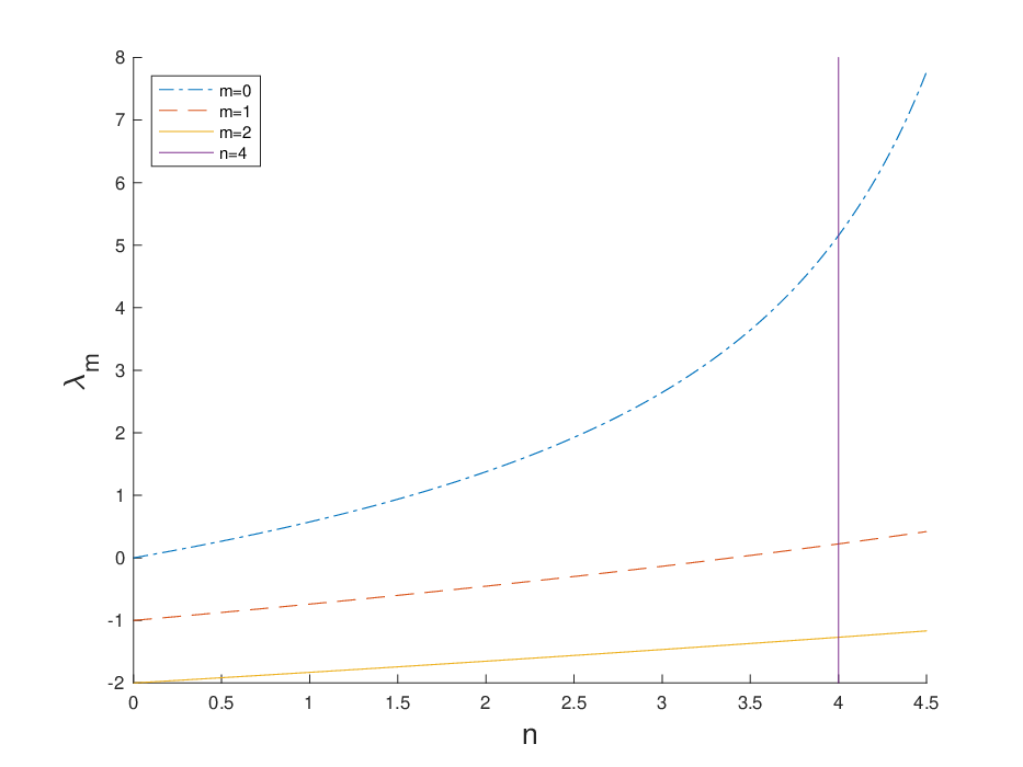
Using (33), when the largest Steklov eigenvalues are
| (34) |
and when the complex Steklov eigenvalues with largest imaginary parts are
| (35) |
5.1 Selfadjoint Cases
When the index of refraction is real, the problem is selfadjoint and all Steklov eigenvalues are real. We compute the six largest Steklov eigenvalues for on a series of uniformly refined meshes for each domain. The results are shown in Tables 1, 2, and 3. The mesh sizes are denoted by . The values are consistent with those in [12].
| 1st | 2nd | 3rd | 4th | 5th | 6th | |
|---|---|---|---|---|---|---|
| 0.2341 | 5.016606 | 0.206380 | 0.205917 | -1.294039 | -1.294339 | -2.561531 |
| 0.1208 | 5.116979 | 0.219175 | 0.219048 | -1.275370 | -1.275440 | -2.494866 |
| 0.0613 | 5.143045 | 0.222469 | 0.222436 | -1.270670 | -1.270687 | -2.478245 |
| 0.0309 | 5.149636 | 0.223301 | 0.223292 | -1.269493 | -1.269497 | -2.474088 |
| 0.0155 | 5.151289 | 0.223509 | 0.223507 | -1.269198 | -1.269199 | -2.473049 |
Note that for the unit disk, the first eigenvalues are given by (33) for . The values of the columns 2, 3, 4 in Table 1 approximate the intersections of and in Fig. 1.
| 1st | 2nd | 3rd | 4th | 5th | 6th | |
|---|---|---|---|---|---|---|
| 0.2441 | 2.191504 | -0.220113 | -0.220397 | -0.929022 | -2.856629 | -2.970847 |
| 0.1220 | 2.199625 | -0.214254 | -0.214327 | -0.913327 | -2.791699 | -2.819631 |
| 0.0610 | 2.201774 | -0.212756 | -0.212774 | -0.909377 | -2.774697 | -2.781648 |
| 0.0305 | 2.202323 | -0.212378 | -0.212383 | -0.908387 | -2.770389 | -2.772125 |
| 0.0153 | 2.202461 | -0.212284 | -0.212285 | -0.908139 | -2.769308 | -2.769742 |
| 1st | 2nd | 3rd | 4th | 5th | 6th | |
|---|---|---|---|---|---|---|
| 0.2383 | 2.507719 | 0.840066 | 0.117326 | -1.103880 | -1.112608 | -1.464999 |
| 0.1192 | 2.526360 | 0.851538 | 0.122637 | -1.090066 | -1.096900 | -1.429175 |
| 0.0596 | 2.531439 | 0.855499 | 0.124041 | -1.086500 | -1.092730 | -1.420001 |
| 0.0298 | 2.532762 | 0.856926 | 0.124402 | -1.085600 | -1.091620 | -1.417681 |
| 0.0149 | 2.533099 | 0.857457 | 0.124494 | -1.085374 | -1.091319 | -1.417098 |
In Fig. 2, we show the convergence rates of Steklov eigenvalues of three domains. Since we use the linear Lagrange finite element, the second order convergence is achieved for the unit circle and the square. For the L-shaped domain, which is non-convex, the convergence rate of the second Steklov eigenvalue is lower than , while the other eigenvalues have second order convergence.

|

|

|
Note that the convergence rate of the eigenvalues relates to the regularity of the associated eigenfunctions. The result in Fig. 2 implies that the eigenfunction associated with the second eigenvalues does not belong to .
5.2 Non-selfadjoint Cases
When is complex, the solution operator is non-selfadjoint. Consequently, we end up with non-Hermitian matrix eigenvalue problem. Computation of complex eigenvalues of non-Hermitian matrices are challenging, in particular, when there is no a priori spectral information on the number and distribution of eigenvalues. To this end, we use the new spectral indicator method introduced in the previous section to compute Steklov eigenvalues. For all examples, we take .
The left picture of Fig. 3 shows the distribution of Steklov eigenvalues for the unit disk on the complex plane. These are eigenvalues computed using Matlab ‘eig’ for the non-Hermitian matrix () resulting from the finite element method. The mesh size is . Note that ‘eig’ is a direct eigensolver and not suitable for larger matrices.

|

|
Since we are interested in eigenvalues close to the origin, we choose the search region on the complex plane to be the square . The right picture of Fig. 3 shows how S-RIM explores and finds the eigenvalues inside .
The computed complex eigenvalues for the three domains are shown in Tables 4, 5, and 6, respectively. We arrange the eigenvalues according to the decreasing order of their imaginary parts. Again, these values are consistent with the values given in [12], which are reconstructed by some inverse algorithm using scattering data.
| 1st | 2nd | 3rd | 4th | |
|---|---|---|---|---|
| 0.2341 | ||||
| 0.1208 | ||||
| 0.0613 | ||||
| 0.0310 | ||||
| 0.0155 |
| 1st | 2nd | 3rd | 4th | |
|---|---|---|---|---|
| 0.2441 | ||||
| 0.1220 | ||||
| 0.0610 | ||||
| 0.0305 | ||||
| 0.0151 |
| 1st | 2nd | 3rd | 4th | |
|---|---|---|---|---|
| 0.2383 | ||||
| 0.1192 | ||||
| 0.0596 | ||||
| 0.0298 | ||||
| 0.0149 |
In Fig. 4, we show the convergence rates of complex Steklov eigenvalues. The second order convergence is achieved for the unit circle and square. Similar to real , the second eigenvalue of the L-shaped domain has lower convergence rate indicating that the associated eigenfunction has lower regularity.

|

|

|
6 Conclusions and Future Works
In this paper, we study the computation of a non-selfadjoint Steklov eigenvalue problem arising from the inverse scattering theory. To the authors’ knowledge, this is the first numerical paper containing both theory and numerical examples. An early paper by Bramble and Osborn considered a similar but different non-selfadjoint Steklov eigenvalue problem [9]. The second order non-selfadjoint operator is assumed to be uniformly elliptic and no numerical results were reported therein.
The contribution of the paper is as follows. The convergence of Lagrange finite elements is proved using the spectral perturbation theory for compact operators. Due to the fact that the problem is non-selfadjoint and no a priori spectral information is available, the recently developed spectral indicator method RIM is considered for the resulting non-Hermitian matrix eigenvalue problems. To improve efficiency, we derive an equivalent but much smaller matrix eigenvalue problem involving only boundary unknowns. Then a modified version of RIM is developed to compute (complex) eigenvalues.
Non-selfadjoint Steklov eigenvalue problems have many important applications. Numerical computation of these problems is challenging. The problem considered in this paper is related to the Helmholtz equation. Similar problems exist for the Maxwell equation and elasticity equation. In future, we plan to extend the theory and algorithm here to these problems.
References
- [1] M.G. Armentano and C. Padra, A posteriori error estimates for the Steklov eigenvalue problem. Appl. Numer. Math. 58 (2008), no. 5, 593-601.
- [2] J. An, H. Bi, and Z. Luo, A highly efficient spectral-Galerkin method based on tensor product for fourth-order Steklov equation with boundary eigenvalue. J. Inequal. Appl. 2016, Paper No. 211, 12 pp.
- [3] A.B. Andreev and T.D. Todorov, Isoparametric finite-element approximation of a Steklov eigenvalue problem. IMA J. Numer. Anal. 24 (2004), no. 2, 309-322.
- [4] I. Babuška and J. Osborn, Eigenvalue Problems, Handbook of Numerical Analysis, Vol. II, Finite Element Methods (Part 1), Edited by P.G. Ciarlet and J.L. Lions, Elseveier Science Publishers B.V. (North-Holland), 1991.
- [5] W.J. Beyn, An integral method for solving nonlinear eigenvalue problems. Linear Algebra Appl. 436 (2012), no. 10, 3839–3863.
- [6] H. Bi, H. Li, and Y. Yang, An adaptive algorithm based on the shifted inverse iteration for the Steklov eigenvalue problem. Appl. Numer. Math. 105 (2016), 64-81.
- [7] H. Bi, Z. Li, and Y. Yang, Local and parallel finite element algorithms for the Steklov eigenvalue problem. Numer. Methods Partial Differential Equations 32 (2016), no. 2, 399-417.
- [8] D. Boffi, Finite element approximation of eigenvalue problems. Acta Numer. 19 (2010), 1-120.
- [9] J.H. Bramble and J.E. Osborn, Approximation of Steklov eigenvalues of non-selfadjoint second order elliptic operators. The mathematical foundations of the finite element method with applications to partial differential equations (Proc. Sympos., Univ. Maryland, Baltimore, Md., 1972), 387-408. Academic Press, New York.
- [10] J.H. Bramble and J.E. Osborn, Rate of convergence estimates for nonselfadjoint eigenvalue approximations. Math. Comp. 27 (1973), 525-549.
- [11] S.C. Brenner and L.R. Scott, The mathematical theory of finite element methods. Third edition. Texts in Applied Mathematics, 15. Springer, New York, 2008.
- [12] F. Cakoni, D. Colton, S. Meng, and P. Monk, Stekloff eigenvalues in inverse scattering. SIAM J. Appl. Math. 76 (2016), no. 4, 1737-1763.
- [13] J. A. Canavati and A. A. Minzoni, A discontinuous Steklov problem with an application to water waves. J. Math. Anal. Appl. 69 (1979), no. 2, 540-558.
- [14] L. Cao, L. Zhang, W. Allegretto, and Y. Lin, Multiscale asymptotic method for Steklov eigenvalue equations in composite media. SIAM J. Numer. Anal. 51 (2013), no. 1, 273-296.
- [15] D. Colton, P. Monk and J. Sun, Analytical and computational methods for transmission eigenvalues, Inverse Problems, Vol. 26 (2010) No. 4, 045011.
- [16] A. Dello Russo and A.E. Alonso, A posteriori error estimates for nonconforming approximations of Steklov eigenvalue problems. Comput. Math. Appl. 62 (2011), no. 11, 4100-4117.
- [17] P. Grisvard, Elliptic Problems in Non Smooth Domains, Pitman, Boston, 1985.
- [18] G.C. Hsiao, W.L. Wendland, Boundary integral equations. Applied Mathematical Sciences, 164. Springer-Verlag, Berlin, 2008.
- [19] R. Huang, A. Struthers, J. Sun and R. Zhang, Recursive integral method for transmission eigenvalues. Journal of Computational Physics, Vol. 327 (2016), 830-840.
- [20] R. Huang, J. Sun and C. Yang, Recursive Integral Method with Cayley Transformation - arXiv preprint arXiv:1705.01646, submitted.
- [21] S. Jia, F. Luo, and H. Xie, A posterior error analysis for the nonconforming discretization of Stokes eigenvalue problem. Acta Math. Sin. (Engl. Ser.) 30 (2014), no. 6, 949-967.
- [22] T. Kato, Perturbation Theory of Linear Operators, Classics in Mathematics, Springer-Verlag, Berlin, 1995.
- [23] P. Kumar and M. Kumar, Simulation of a nonlinear Steklov eigenvalue problem using finite-element approximation. Comput. Math. Model. 21 (2010), no. 1, 109-116.
- [24] N. Kuznetsov, T. Kulczycki, M. Kwaśnicki, A. Nazarov, S. Poborchi, I. Polterovich, and B. Siudeja, The legacy of Vladimir Andreevich Steklov. Notices Amer. Math. Soc. 61 (2014), no. 1, 9-22.
- [25] D. Mora, G. Rivera, and R. Rodríguez, A virtual element method for the Steklov eigenvalue problem. Math. Models Methods Appl. Sci. 25 (2015), no. 8, 1421-1445.
- [26] J. Osborn, Spectral Approximation for Compact Operators Mathematics of Computation, Vol. 29 (1975), No. 131, 712–725.
- [27] E. Polizzi, Density-matrix-based algorithms for solving eigenvalue problems. Phys. Rev. B., 79(2009), 115112 .
- [28] Y. Saad, Numerical Methods for Large Eigenvalue Problems, Classics in Applied Mathematics, 66. Society for Industrial and Applied Mathematics, Philadelphia, 2011.
- [29] T. Sakurai and H. Sugiura, A projection method for generalized eigenvalue problems using numerical integration. J. Comput. Appl. Math., 159 (2003), no. 1, 119–128.
- [30] J. Sun, Iterative methods for transmission eigenvalues. SIAM J. Numer. Anal., 49(5),1860-1874, 2011.
- [31] J. Sun and A. Zhou, Finite element methods for eigenvalue problems. CRC Press, Taylor & Francis Group, Boca Raton, London, New York, 2016.
- [32] H. Xie, A type of multilevel method for the Steklov eigenvalue problem. IMA Journal of Numerical Analysis, Vol. 34 (2014), 592-608.