跳到论文正文
W Papers独立论文阅读器 arXiv:1804.02393 论文正文 计算阅读时间 · 0%
引用这篇论文根据当前论文元数据生成,正式投稿前建议核对。


License: arXiv.org perpetual non-exclusive license
arXiv:1804.02393v1 [cs.AI] 06 Apr 2018

Formal Ways for Measuring Relations between Concepts in Conceptual SpacesThanks: This article is a revised and considerably extended version of a conference paper presented at SGAI 2017 [Bechberger and Kühnberger, 2017b].

Lucas Bechberger 🖂(0000-0002-1962-1777)    Kai-Uwe Kühnberger E-mail kai-uwe.kuehnberger@uni-osnabrueck.de Affiliation: Institute of Cognitive Science, Osnabrück University, Osnabrück, Germany , E-mail lucas.bechberger@uni-osnabrueck.de
Abstract

The highly influential framework of conceptual spaces provides a geometric way of representing knowledge. Instances are represented by points in a high-dimensional space and concepts are represented by regions in this space. In this article, we extend our recent mathematical formalization of this framework by providing quantitative mathematical definitions for measuring relations between concepts: We develop formal ways for computing concept size, subsethood, implication, similarity, and betweenness. This considerably increases the representational capabilities of our formalization and makes it the most thorough and comprehensive formalization of conceptual spaces developed so far. onceptual Spaces ·  Fuzzy Sets ·  Concept Size ·  Subsethood ·  Implication ·  Similarity ·  Betweenness

Keywords: 
C

1 Introduction

One common criticism of symbolic AI approaches is that the symbols they operate on do not contain any meaning: For the system, they are just arbitrary tokens that can be manipulated in some way. This lack of inherent meaning in abstract symbols is called the “symbol grounding problem” [Harnad, 1990]. One approach towards solving this problem is to devise a grounding mechanism that connects abstract symbols to the real world, i.e., to perception and action.

The cognitive framework of conceptual spaces [Gärdenfors, 2000, Gärdenfors, 2014] attempts to bridge this gap between symbolic and subsymbolic AI by proposing an intermediate conceptual layer based on geometric representations. A conceptual space is a similarity space spanned by a number of quality dimensions that are based on perception and/or subsymbolic processing. Regions in this space correspond to concepts and can be referred to as abstract symbols.

The framework of conceptual spaces has been highly influential in the last 15 years within cognitive science [Douven et al., 2011, Fiorini et al., 2013, Lieto et al., 2017]. It has also sparked considerable research in various subfields of artificial intelligence, ranging from robotics and computer vision [Chella et al., 2003] over the semantic web [Adams and Raubal, 2009b] to plausible reasoning [Derrac and Schockaert, 2015].

One important aspect of conceptual representations is however often ignored by these research efforts: Typically, the different features of a concept are correlated with each other. For instance, there is an obvious correlation between the color and the taste of an apple: Red apples tend to be sweet and green apples tend to be sour. Recently, we have proposed a formalization of the conceptual spaces framework that is capable of representing such correlations in a geometric way [Bechberger and Kühnberger, 2017a]. Our formalization not only contains a parametric definition of concepts, but also different operations to create new concepts from old ones (namely: intersection, unification, and projection).

In this article, we provide mathematical definitions for the notions of concept size, subsethood, implication, similarity, and betweenness. This considerably increases the representational power of our formalization by introducing measurable ways of describing relations between concepts.

The remainder of this article is structured as follows: Section 2 introduces the general framework of conceptual spaces along with our recent formalization. In Section 3, we extend this formalization with additional operations and in Section 4 we provide an illustrative example. Section 5 contains a summary of related work and Section 6 concludes the paper.

2 Conceptual Spaces

This section presents the cognitive framework of conceptual spaces as described by [Gärdenfors, 2000] and as formalized by [Bechberger and Kühnberger, 2017a].

2.1 Dimensions, Domains, and Distance

A conceptual space is a similarity space spanned by a set DD of so-called “quality dimensions”. Each of these dimensions d∈Dd\in D represents an interpretable way in which two stimuli can be judged to be similar or different. Examples for quality dimensions include temperature, weight, time, pitch, and hue. The distance between two points xx and yy with respect to a dimension dd is denoted as |xd−yd||x_{d}-y_{d}|.

A domain δ⊆D\delta\subseteq D is a set of dimensions that inherently belong together. Different perceptual modalities (like color, shape, or taste) are represented by different domains. The color domain for instance consists of the three dimensions hue, saturation, and brightness. Distance within a domain δ\delta is measured by the weighted Euclidean metric dEd_{E}.

The overall conceptual space C​SCS is defined as the product space of all dimensions. Distance within the overall conceptual space is measured by the weighted Manhattan metric dMd_{M} of the intra-domain distances. This is supported by both psychological evidence [Attneave, 1950, Shepard, 1964, Johannesson, 2001] and mathematical considerations [Aggarwal et al., 2001]. Let Δ\Delta be the set of all domains in C​SCS. The combined distance dCΔd_{C}^{\Delta} within C​SCS is defined as follows:

dCΔ​(x,y,W)=∑δ∈Δwδ⋅∑d∈δwd⋅|xd−yd|2d_{C}^{\Delta}(x,y,W)=\sum_{\delta\in\Delta}w_{\delta}\cdot\sqrt{\sum_{d\in\delta}w_{d}\cdot|x_{d}-y_{d}|^{2}}

The parameter W=⟨WΔ,{Wδ}δ∈Δ⟩W=\langle W_{\Delta},\{W_{\delta}\}_{\delta\in\Delta}\rangle contains two parts: WΔW_{\Delta} is the set of positive domain weights wδw_{\delta} with ∑δ∈Δwδ=|Δ|\textstyle\sum_{\delta\in\Delta}w_{\delta}=|\Delta|. Moreover, WW contains for each domain δ∈Δ\delta\in\Delta a set WδW_{\delta} of dimension weights wdw_{d} with ∑d∈δwd=1\textstyle\sum_{d\in\delta}w_{d}=1.

The similarity of two points in a conceptual space is inversely related to their distance. This can be written as follows :

Sim(x,y)=e−c⋅d(x,y)with a constantc>0and a given metricdSim(x,y)=e^{-c\cdot d(x,y)}\quad\text{with a constant}\;c>0\;\text{and a given metric}\;d

Betweenness is a logical predicate B⁡(x,y,z)B(x,y,z) that is true if and only if yy is considered to be between xx and zz. It can be defined based on a given metric dd:

Bd​(x,y,z):⇔d⁡(x,y)+d⁡(y,z)=d⁡(x,z)B_{d}(x,y,z):\iff d(x,y)+d(y,z)=d(x,z)

The betweenness relation based on dEd_{E} results in the line segment connecting the points xx and zz, whereas the betweenness relation based on dMd_{M} results in an axis-parallel cuboid between the points xx and zz. One can define convexity and star-shapedness based on the notion of betweenness:

Definition 1

(Convexity)
A set C⊆C​SC\subseteq CS is convex under a metric d:⇔d\;:\iff

∀x∈C,z∈C,y∈C​S:(Bd​(x,y,z)→y∈C)\forall{x\in C,z\in C,y\in CS}:\left(B_{d}(x,y,z)\rightarrow y\in C\right)

Definition 2

(Star-shapedness)
A set S⊆C​SS\subseteq CS is star-shaped under a metric dd with respect to a set P⊆S:⇔P\subseteq S\;:\iff

∀p∈P,z∈S,y∈C​S:(Bd​(p,y,z)→y∈S)\forall{p\in P,z\in S,y\in CS}:\left(B_{d}(p,y,z)\rightarrow y\in S\right)

2.2 Properties and Concepts

[Gärdenfors, 2000] observes that properties like “red”, “round”, and “sweet” can be defined on individual domains (e.g., color, shape, taste), whereas full-fleshed concepts like “apple” or “dog” involve multiple domains. Each domain involved in representing a concept has a certain importance, which is reflected by so-called “salience weights”. Another important aspect of concepts are the correlations between the different domains, which are important for both learning [Billman and Knutson, 1996] and reasoning [Murphy, 2002, Ch 8].

Based on the principle of cognitive economy, Gärdenfors argues that both properties and concepts should be represented as convex sets. However, as we demonstrated in [Bechberger and Kühnberger, 2017a], one cannot geometrically encode correlations between domains when using convex sets: The left part of Figure 1 shows two domains (age and height) with an intuitive sketch for the concepts of child and adult. As domains are combined with the Manhattan metric, a convex set corresponds in this case to an axis-parallel cuboid. One can easily see that this convex representation (middle part of Figure 1) is not satisfactory, because the correlation of the two domains is not encoded. We therefore proposed in [Bechberger and Kühnberger, 2017a] to relax the convexity criterion and to use star-shaped sets, which is illustrated in the right part of Figure 1. This enables a geometric representation of correlations while still being only a minimal departure from the original framework.

Refer to caption
Figure 1: Left: Intuitive way to define regions for the concepts of “adult” and “child”. Middle: Representation by using convex sets. Right: Representation by using star-shaped sets with central points marked by crosses.

We have based our formalization on axis-parallel cuboids that can be described by a triple ⟨ΔC,p−,p+⟩\langle\Delta_{C},p^{-},p^{+}\rangle consisting of a set of domains ΔC\Delta_{C} on which this cuboid CC is defined and two points p−p^{-} and p+p^{+}, such that

x∈C⇔∀δ∈ΔC:∀d∈δ:pd−≤xd≤pd+x\in C\iff\forall{\delta\in\Delta_{C}}:\forall{d\in\delta}:p_{d}^{-}\leq x_{d}\leq p_{d}^{+}

These cuboids are convex under dCΔd_{C}^{\Delta}. It is also easy to see that any union of convex sets that have a non-empty intersection is star-shaped [Smith, 1968]. We define the core of a concept as follows:

Definition 3

(Simple star-shaped set)
A simple star-shaped set SS is described as a tuple ⟨ΔS,{C1,…,Cm}⟩\langle\Delta_{S},\{C_{1},\dots,C_{m}\}\rangle. ΔS⊆Δ\Delta_{S}\subseteq\Delta is a set of domains on which the cuboids {C1,…,Cm}\{C_{1},\dots,C_{m}\} (and thus also SS) are defined. Moreover, it is required that the central region P:=⋂i=1mCi≠∅P:=\textstyle\bigcap_{i=1}^{m}C_{i}\neq\emptyset. Then the simple star-shaped set SS is defined as

S:=⋃i=1mCiS:=\bigcup_{i=1}^{m}C_{i}

In order to represent imprecise concept boundaries, we use fuzzy sets [Zadeh, 1965, Bělohlávek and Klir, 2011]. A fuzzy set is characterized by its membership function μ:C​S→[0,1]\mu:CS\rightarrow[0,1] that assigns a degree of membership to each point in the conceptual space. The membership of a point to a fuzzy concept is based on its maximal similarity to any of the points in the concept’s core:

Definition 4

(Fuzzy simple star-shaped set)
A fuzzy simple star-shaped set S~\widetilde{S} is described by a quadruple ⟨S,μ0,c,W⟩\langle S,\mu_{0},c,W\rangle where S=⟨ΔS,{C1,…,Cm}⟩S=\langle\Delta_{S},\{C_{1},\dots,C_{m}\}\rangle is a non-empty simple star-shaped set. The parameter μ0∈(0,1]\mu_{0}\in(0,1] controls the highest possible membership to S~\widetilde{S} and is usually set to 1. The sensitivity parameter c>0c>0 controls the rate of the exponential decay in the similarity function. Finally, W=⟨WΔS,{Wδ}δ∈ΔS⟩W=\langle W_{\Delta_{S}},\{W_{\delta}\}_{\delta\in\Delta_{S}}\rangle contains positive weights for all domains in ΔS\Delta_{S} and all dimensions within these domains, reflecting their respective importance. We require that ∑δ∈ΔSwδ=|ΔS|\textstyle\sum_{\delta\in\Delta_{S}}w_{\delta}=|\Delta_{S}| and that ∀δ∈ΔS:∑d∈δwd=1\forall{\delta\in\Delta_{S}}:\textstyle\sum_{d\in\delta}w_{d}=1. The membership function of S~\widetilde{S} is then defined as follows:

μS~(x)=μ0⋅maxy∈S(e−c⋅dCΔ(x,y,W))\mu_{\widetilde{S}}(x)=\mu_{0}\cdot\max_{y\in S}\left(e^{-c\cdot d_{C}^{\Delta}(x,y,W)}\right)

The sensitivity parameter cc controls the overall degree of fuzziness of S~\widetilde{S} by determining how fast the membership drops to zero. The weights WW represent not only the relative importance of the respective domain or dimension for the represented concept, but they also influence the relative fuzziness with respect to this domain or dimension. Note that if |ΔS|=1|\Delta_{S}|=1, then S~\widetilde{S} represents a property, and if |ΔS|>1|\Delta_{S}|>1, then S~\widetilde{S} represents a concept. Figure 2 illustrates this definition (the xx and yy axes are assumed to belong to different domains and are combined with dMd_{M} using equal weights).

Refer to caption
Figure 2: Left: Three cuboids C1,C2,C3C_{1},C_{2},C_{3} with nonempty intersection. Middle: Resulting simple star-shaped set SS based on these cuboids. Right: Fuzzy simple star-shaped set S~\tilde{S} based on SS with three α\alpha-cuts for α∈{1.0,0.5,0.25}\alpha\in\{1.0,0.5,0.25\}.

In our previous work [Bechberger and Kühnberger, 2017a], we have also provided a number of operations, which can be used to create new concepts from old ones, namely intersection, unification, and projection: The intersection of two concepts can be interpreted as the logical “and” – e.g., intersecting the property “green” with the concept “banana” results in the set of all objects that are both green and bananas. The unification of two concepts can be used to construct more abstract categories (e.g., defining “fruit” as the unification of “apple”, “banana”, “coconut”, etc.). Projecting a concept onto a subspace corresponds to focusing on certain domains while completely ignoring others.

3 Defining Additional Operations

3.1 Concept Size

The size of a concept gives an intuition about its specificity: Large concepts are more general and small concepts are more specific. This is one obvious aspect in which one can compare two concepts to each other.

One can use a measure MM to describe the size of a fuzzy set. It can be defined in our context as follows (cf. [Bouchon-Meunier et al., 1996]):

Definition 5

A measure MM on a conceptual space C​SCS is a function M:ℱ⁡(C​S)→ℝ0+M:\mathcal{F}(CS)\rightarrow\mathbb{R}^{+}_{0} with M⁡(∅)=0M(\emptyset)=0 and A~⊆B~⇒M⁡(A~)≤M⁡(B~)\widetilde{A}\subseteq\widetilde{B}\Rightarrow M(\widetilde{A})\leq M(\widetilde{B}), where ℱ⁡(C​S)\mathcal{F}(CS) is the fuzzy power set of C​SCS and where A~⊆B~:⇔∀x∈C​S:μA~​(x)≤μB~​(x)\widetilde{A}\subseteq\widetilde{B}:\iff\forall{x\in CS}:\mu_{\widetilde{A}}(x)\leq\mu_{\widetilde{B}}(x).

A common measure for fuzzy sets is the integral over the set’s membership function, which is equivalent to the Lebesgue integral over the fuzzy set’s α\alpha-cuts:

M⁡(A~):=∫C​SμA~​(x)​𝑑x=∫01V⁡(A~α)​𝑑αM(\widetilde{A}):=\int_{CS}\mu_{\widetilde{A}}(x)\;dx=\int_{0}^{1}V(\widetilde{A}^{\alpha})\;d\alpha (1)

We use V⁡(A~α)V(\widetilde{A}^{\alpha}) to denote the volume of a fuzzy set’s α\alpha-cut A~α={x∈C​S|μA~​(x)≥α}\widetilde{A}^{\alpha}=\{x\in CS\;|\;\mu_{\widetilde{A}}(x)\geq\alpha\}. We define for each cuboid Ci∈SC_{i}\in S its fuzzified version C~i\widetilde{C}_{i} (cf. Definition 4):

μC~i(x)=μ0⋅maxy∈Ci(e−c⋅dCΔ(x,y,W))\mu_{\widetilde{C}_{i}}(x)=\mu_{0}\cdot\max_{y\in C_{i}}\left(e^{-c\cdot d_{C}^{\Delta}(x,y,W)}\right)

It is obvious that μS~​(x)=maxCi∈S⁡μC~i​(x)\mu_{\widetilde{S}}(x)=\max_{C_{i}\in S}\mu_{\widetilde{C}_{i}}(x). It is also clear that the intersection of two fuzzified cuboids is again a fuzzified cuboid. Finally, one can easily see that we can use the inclusion-exclusion formula (cf. e.g., [Bogart, 1989]) to compute the overall measure of S~\widetilde{S} based on the measure of its fuzzified cuboids:

M⁡(S~)=∑l=1m((−1)l+1⋅∑{i1,…,il}⊆{1,…,m}M⁡(⋂i∈{i1,…,il}C~i))M(\widetilde{S})=\sum_{l=1}^{m}\left((-1)^{l+1}\cdot\sum_{\begin{subarray}{c}\{i_{1},\dots,i_{l}\}\\ \subseteq\{1,\dots,m\}\end{subarray}}M\left(\bigcap_{i\in\{i_{1},\dots,i_{l}\}}\widetilde{C}_{i}\right)\right) (2)

The outer sum iterates over the number of cuboids under consideration (with mm being the total number of cuboids in S) and the inner sum iterates over all sets of exactly ll cuboids. The overall formula generalizes the observation that |C~1∪C~2|=|C~1|+|C~2|−|C~1∩C~2||\widetilde{C}_{1}\cup\widetilde{C}_{2}|=|\widetilde{C}_{1}|+|\widetilde{C}_{2}|-|\widetilde{C}_{1}\cap\widetilde{C}_{2}| from two to mm sets.

In order to derive M⁡(S~)M(\widetilde{S}), we first describe how to compute V⁡(C~α)V(\widetilde{C}^{\alpha}), i.e., the size of a fuzzified cuboid’s α\alpha-cut. Using Equation 1, we can then derive M⁡(C~)M(\widetilde{C}), which we can in turn insert into Equation 2 to compute the overall size of S~\widetilde{S}.

Figure 3 illustrates the α\alpha-cut of a fuzzified two-dimensional cuboid both under dEd_{E} (left) and under dMd_{M} (right). Because the membership function is defined based on an exponential decay, one can interpret each α\alpha-cut as an ϵ\epsilon-neighborhood of the original cuboid C, where ϵ\epsilon depends on α\alpha:

x∈C~α⇔μ0⋅maxy∈C(e−c⋅dCΔ(x,y,W))≥α⇔miny∈CdCΔ(x,y,W)≤−1c⋅ln(αμ0)x\in{\widetilde{C}}^{\alpha}\iff\mu_{0}\cdot\max_{y\in C}\left(e^{-c\cdot d_{C}^{\Delta}(x,y,W)}\right)\geq\alpha\iff\min_{y\in C}d_{C}^{\Delta}(x,y,W)\leq-\frac{1}{c}\cdot\ln\left(\frac{\alpha}{\mu_{0}}\right)
Refer to caption
Figure 3: α\alpha-cut of a fuzzified cuboid under dEd_{E} (left) and dMd_{M} (right), respectively.

V⁡(C~α)V(\widetilde{C}^{\alpha}) can be described as a sum of different components. Let us use the shorthand notation bd:=pd+−pd−b_{d}:=p_{d}^{+}-p_{d}^{-}. Looking at Figure 3, one can see that all components of V⁡(C~α)V(\widetilde{C}^{\alpha}) can be described by ellipses: Component I is a zero-dimensional ellipse (i.e., a point) that was extruded in two dimensions with extrusion lengths of b1b_{1} and b2b_{2}, respectively. Component II consists of two one-dimensional ellipses (i.e., line segments) that were extruded in one dimension, and component III is a two-dimensional ellipse. Note that ellipses under dMd_{M} have the form of streched diamonds.

Let us denote by Δ{d1,…,di}\Delta_{\{d_{1},\dots,d_{i}\}} the domain structure obtained by eliminating from Δ\Delta all dimensions d∈D∖{d1,…,di}d\in D\setminus\{d_{1},\dots,d_{i}\}. Moreover, let V⁡(r,Δ,W)V(r,\Delta,W) be the hypervolume of a hyperball under dCΔ​(⋅,⋅,W)d_{C}^{\Delta}(\cdot,\cdot,W) with radius rr. In this case, a hyperball is the set of all points with a distance of at most rr (measured by dCΔ​(⋅,⋅,W)d_{C}^{\Delta}(\cdot,\cdot,W)) to a central point. Note that the weights WW will cause this ball to have the form of an ellipse. For instance, in Figure 3, we assume that wd1<wd2w_{d_{1}}<w_{d_{2}} which means that we allow larger differences with respect to d1d_{1} than with respect to d2d_{2}. This causes the hyperballs to be streched in the d1d_{1} dimension, thus obtaining the shape of an ellipse. We can in general describe V⁡(C~α)V(\widetilde{C}^{\alpha}) as follows:

V(C~α)=∑i=0n(∑{d1,…,di}⊆D(∏d∈D∖{d1,…,di}bd)⋅V(−1c⋅ln(αμ0),Δ{d1,…,di},W))V(\widetilde{C}^{\alpha})=\sum_{i=0}^{n}\left(\sum_{\begin{subarray}{c}\{d_{1},\dots,d_{i}\}\\ \subseteq D\end{subarray}}\left(\prod_{\begin{subarray}{c}d\in\\ D\setminus\{d_{1},\dots,d_{i}\}\end{subarray}}b_{d}\right)\cdot V\left(-\frac{1}{c}\cdot\ln\left(\frac{\alpha}{\mu_{0}}\right),\Delta_{\{d_{1},\dots,d_{i}\}},W\right)\right)

The outer sum of this formula runs over the number of dimensions with respect to which a given point x∈C~αx\in\widetilde{C}^{\alpha} lies outside of CC. We then sum over all combinations {d1,…,di}\{d_{1},\dots,d_{i}\} of dimensions for which this could be the case, compute the volume V⁡(⋅,⋅,⋅)V(\cdot,\cdot,\cdot) of the ii-dimensional hyperball under these dimensions and extrude this intermediate result in all remaining dimensions by multiplying with ∏d∈D∖{d1,…,di}bd\prod_{d\in D\setminus\{d_{1},\dots,d_{i}\}}b_{d}.

Let us illustrate this formula for the α\alpha-cuts shown in Figure 3: For i=0i=0, we can only select the empty set for the inner sum, so we end up with b1⋅b2b_{1}\cdot b_{2}, which is the size of the original cuboid (i.e., component I). For i=1i=1, we can either pick {d1}\{d_{1}\} or {d2}\{d_{2}\} in the inner sum. For {d1}\{d_{1}\}, we compute the size of the left and right part of component II by multiplying V(−1c⋅ln(αμ0),Δ{d1},W)V\left(-\frac{1}{c}\cdot\ln\left(\frac{\alpha}{\mu_{0}}\right),\Delta_{\{d_{1}\}},W\right) (i.e., their combined width) with b2b_{2} (i.e., their height). For {d2}\{d_{2}\}, we analogously compute the size of the upper and the lower part of component II. Finally, for i=2i=2, we can only pick {d1,d2}\{d_{1},d_{2}\} in the inner sum, leaving us with V(−1c⋅ln(αμ0),Δ,W)V\left(-\frac{1}{c}\cdot\ln\left(\frac{\alpha}{\mu_{0}}\right),\Delta,W\right), which is the size of component III. One can easily see that the formula for V⁡(C~α)V(\widetilde{C}^{\alpha}) also generalizes to higher dimensions.

Proposition 1

V⁡(r,Δ,W)=1∏δ∈Δwδ⋅∏d∈δwd⋅rnn!⋅∏δ∈Δ(|δ|!⋅π|δ|2Γ⁡(|δ|2+1))V(r,\Delta,W)=\frac{1}{\prod_{\delta\in\Delta}w_{\delta}\cdot\prod_{d\in\delta}\sqrt{w_{d}}}\cdot\frac{r^{n}}{n!}\cdot\prod_{\delta\in\Delta}\left(|\delta|!\cdot\frac{\pi^{\frac{|\delta|}{2}}}{\Gamma\left(\frac{|\delta|}{2}+1\right)}\right)

Proof

See Appendix A. ∎

Defining δ⁡(d)\delta(d) as the unique δ∈Δ\delta\in\Delta with d∈δd\in\delta, and ad:=wδ⁡(d)⋅wd⋅bd⋅ca_{d}:=w_{\delta(d)}\cdot\sqrt{w_{d}}\cdot b_{d}\cdot c, we can use Proposition 1 to rewrite V⁡(C~α)V(\widetilde{C}^{\alpha}):

V⁡(C~α)\displaystyle V(\widetilde{C}^{\alpha}) =1cn​∏d∈Dwδ⁡(d)​wd∑i=0n((−1)i⋅ln⁡(αμ0)ii!⋅∑{d1,…,di}⊆D(∏d∈D∖{d1,…,di}ad)⋅\displaystyle=\frac{1}{c^{n}\prod_{d\in D}w_{\delta(d)}\sqrt{w_{d}}}\sum_{i=0}^{n}\left(\frac{(-1)^{i}\cdot\ln\left(\frac{\alpha}{\mu_{0}}\right)^{i}}{i!}\cdot\sum_{\begin{subarray}{c}\{d_{1},\dots,d_{i}\}\\ \subseteq D\end{subarray}}\left(\prod_{\begin{subarray}{c}d\in\\ D\setminus\{d_{1},\dots,d_{i}\}\end{subarray}}a_{d}\right)\cdot\right.
OPEN∏δ∈Δ{d1,…,di}(|δ|!⋅π|δ|2Γ⁡(|δ|2+1)))\displaystyle\left.\hskip 128.0374pt\prod_{\begin{subarray}{c}\delta\in\\ \Delta_{\{d_{1},\dots,d_{i}\}}\end{subarray}}\left(|\delta|!\cdot\frac{\pi^{\frac{|\delta|}{2}}}{\Gamma\left(\frac{|\delta|}{2}+1\right)}\right)\right)

We can solve Equation 1 to compute M⁡(C~)M(\widetilde{C}) by using the following lemma:

Lemma 1

∀n∈ℕ:∫01ln⁡(x)n​𝑑x=(−1)n⋅n!\forall n\in\mathbb{N}:\int_{0}^{1}\ln(x)^{n}dx=(-1)^{n}\cdot n!

Proof

Substitute x=etx=e^{t} and s=−ts=-t, apply the definition of the Γ\Gamma function. ∎

Proposition 2

The measure of a fuzzified cuboid C~\widetilde{C} can be computed as follows:

M⁡(C~)\displaystyle M(\widetilde{C}) =μ0cn​∏d∈Dwδ⁡(d)​wd∑i=0n(∑{d1,…,di}⊆D(∏d∈D∖{d1,…,di}ad)⋅\displaystyle=\frac{\mu_{0}}{c^{n}\prod_{d\in D}w_{\delta(d)}\sqrt{w_{d}}}\sum_{i=0}^{n}\Bigg(\sum_{\begin{subarray}{c}\{d_{1},\dots,d_{i}\}\\ \subseteq D\end{subarray}}\left(\prod_{\begin{subarray}{c}d\in\\ D\setminus\{d_{1},\dots,d_{i}\}\end{subarray}}a_{d}\right)\cdot
OPEN∏δ∈Δ{d1,…,di}(|δ|!⋅π|δ|2Γ⁡(|δ|2+1)))\displaystyle\hskip 142.26378pt\prod_{\begin{subarray}{c}\delta\in\\ \Delta_{\{d_{1},\dots,d_{i}\}}\end{subarray}}\left(|\delta|!\cdot\frac{\pi^{\frac{|\delta|}{2}}}{\Gamma\left(\frac{|\delta|}{2}+1\right)}\right)\Bigg)
Proof

Substitute x=αμ0x=\frac{\alpha}{\mu_{0}} in Equation 1 and apply Lemma 1. ∎

Note that although the formula for M⁡(C~)M(\widetilde{C}) is quite complex, it can be easily implemented via a set of nested loops. As mentioned earlier, we can use the result from Proposition 2 in combination with the inclusion-exclusion formula (Equation 2) to compute M⁡(S~)M(\widetilde{S}) for any concept S~\widetilde{S}. Also Equation 2 can be easily implemented via a set of nested loops. Note that M⁡(S~)M(\widetilde{S}) is always computed only on ΔS\Delta_{S}, i.e., the set of domains on which S~\widetilde{S} is defined.

3.2 Subsethood

In order to represent knowledge about a hierarchy of concepts, one needs to be able to determine whether one concept is a subset of another concept. For instance, the fact that S~G​r​a​n​n​y​S​m​i​t​h⊆S~a​p​p​l​e\widetilde{S}_{GrannySmith}\subseteq\widetilde{S}_{apple} indicates that Granny Smith is a hyponym of apple.

The classic definition of subsethood for fuzzy sets reads as follows:

S~1⊆S~2:⇔∀x∈C​S:μS~1​(x)≤μS~2​(x)\widetilde{S}_{1}\subseteq\widetilde{S}_{2}:\iff\forall{x\in CS}:\mu_{\widetilde{S}_{1}}(x)\leq\mu_{\widetilde{S}_{2}}(x)

We can derive the following set of necessary and jointly sufficient conditions for subsethood of concepts:

Proposition 3

Let S~1=⟨S1,μ0(1),c(1),W(1)⟩,S~2=⟨S2,μ0(2),c(2),W(2)⟩\widetilde{S}_{1}=\langle S_{1},\mu_{0}^{(1)},c^{(1)},W^{(1)}\rangle,\widetilde{S}_{2}=\langle S_{2},\mu_{0}^{(2)},c^{(2)},W^{(2)}\rangle be two concepts. Then, S~1⊆S~2\widetilde{S}_{1}\subseteq\widetilde{S}_{2} if and only if the following conditions are true:

ΔS2⊆ΔS1\displaystyle\Delta_{S_{2}}\subseteq\Delta_{S_{1}} and ​μ0(1)≤μ0(2)​ and ​S1⊆S~2μ0(1)\displaystyle\text{ and }\mu_{0}^{(1)}\leq\mu_{0}^{(2)}\text{ and }S_{1}\subseteq{\widetilde{S}_{2}}^{\mu_{0}^{(1)}}
and ​∀d∈DS2:c(1)⋅wδ⁡(d)(1)⋅wd(1)≥c(2)⋅wδ⁡(d)(2)⋅wd(2)\displaystyle\text{ and }\forall d\in D_{S_{2}}:c^{(1)}\cdot w^{(1)}_{\delta(d)}\cdot\sqrt{w^{(1)}_{d}}\geq c^{(2)}\cdot w^{(2)}_{\delta(d)}\cdot\sqrt{w^{(2)}_{d}}
Proof

See Appendix B. ∎

Please note that S~1⊆S~2\widetilde{S}_{1}\subseteq\widetilde{S}_{2} either is true or false – which is a binary decision. It is however desirable to define a degree of subsethood in order to make more fine-grained distinctions. Many of the definitions for degrees of subsethood proposed in the fuzzy set literature [Bouchon-Meunier et al., 1996] require that the underlying universe is discrete. The following definition [Kosko, 1992] works also in a continuous space and is conceptually quite straightforward:

S​u​b​(S~1,S~2):=M⁡(S~1∩S~2)M⁡(S~1)with a measure ​MSub(\widetilde{S}_{1},\widetilde{S}_{2}):=\frac{M(\widetilde{S}_{1}\cap\widetilde{S}_{2})}{M(\widetilde{S}_{1})}\quad\text{with a measure }M

One can interpret this definition intuitively as the “percentage of S~1\widetilde{S}_{1} that is also in S~2\widetilde{S}_{2}”. It can be easily implemented based on the measure defined in Section 3.1 and the intersection defined in [Bechberger and Kühnberger, 2017a]. If S~1\widetilde{S}_{1} and S~2\widetilde{S}_{2} are not defined on the same domains, then we first project them onto their shared subset of domains before computing their degree of subsethood.

When computing the intersection of two concepts with different sensitivity parameters c(1),c(2)c^{(1)},c^{(2)} and different weights W(1),W(2)W^{(1)},W^{(2)}, one needs to define new parameters c′c^{\prime} and W′W^{\prime} for the resulting concept. In our earlier work [Bechberger and Kühnberger, 2017a], we have argued that the sensitivity parameter c′c^{\prime} should be set to the minimum of c(1)c^{(1)} and c(2)c^{(2)}. As a larger value for cc causes the membership function to drop faster, this means that the concept resulting from intersecting two imprecise concepts is at least as imprecise as the original concepts. Moreover, we defined the set of new salience weights W′W^{\prime} as a linear interpolation between W(1)W^{(1)} and W(2)W^{(2)}.

Now if c(1)>c(2)c^{(1)}>c^{(2)}, then c′=min⁡(c(1),c(2))=c(2)<c(1)c^{\prime}=\min(c^{(1)},c^{(2)})=c^{(2)}<c^{(1)}. It might thus happen that M⁡(S~1∩S~2)>M⁡(S~1)M(\widetilde{S}_{1}\cap\widetilde{S}_{2})>M(\widetilde{S}_{1}), and that therefore S​u​b​(S~1,S~2)>1Sub(\widetilde{S}_{1},\widetilde{S}_{2})>1. As we would like to confine S​u​b​(S~1,S~2)Sub(\widetilde{S}_{1},\widetilde{S}_{2}) to the interval [0,1][0,1], we should use the same cc and WW for computing both M⁡(S~1∩S~2)M(\widetilde{S}_{1}\cap\widetilde{S}_{2}) and M⁡(S~1)M(\widetilde{S}_{1}).

When judging whether S~1\widetilde{S}_{1} is a subset of S~2\widetilde{S}_{2}, we can think of S~2\widetilde{S}_{2} as setting the context by determining the relative importance of the different domains and dimensions as well as the degree of fuzziness. For instance, when judging whether tomatoes are vegetables, we focus our attention on the features that are crucial to the definition of the “vegetable” concept. We thus propose to use c(2)c^{(2)} and W(2)W^{(2)} when computing M⁡(S~1∩S~2)M(\widetilde{S}_{1}\cap\widetilde{S}_{2}) and M⁡(S~1)M(\widetilde{S}_{1}).

Please note that this ensures that S​u​b​(S~1,S~2)∈[0,1]Sub(\widetilde{S}_{1},\widetilde{S}_{2})\in[0,1] holds. However, by using the same cc and WW for both M⁡(S~1∩S~2)M(\widetilde{S}_{1}\cap\widetilde{S}_{2}) and M⁡(S~1)M(\widetilde{S}_{1}), we lose the guarantee that S​u​b​(S~1,S~2)=1.0⇒S~1⊆S~2Sub(\widetilde{S}_{1},\widetilde{S}_{2})=1.0\Rightarrow\widetilde{S}_{1}\subseteq\widetilde{S}_{2}: Let S~=⟨S,μ0,c,W⟩\widetilde{S}=\langle S,\mu_{0},c,W\rangle be a concept and define S~′:=⟨S,μ0,c′,W⟩\widetilde{S}^{\prime}:=\langle S,\mu_{0},c^{\prime},W\rangle with c′<cc^{\prime}<c. One can easily see that S​u​b​(S~′,S~)=1.0Sub(\widetilde{S}^{\prime},\widetilde{S})=1.0, but that S~′⊈S~\widetilde{S}^{\prime}\not\subseteq\widetilde{S}. In practical applications, however, this is not necessarily a problem: If S​u​b​(S~1,S~2)=1.0Sub(\widetilde{S}_{1},\widetilde{S}_{2})=1.0, we can use Proposition 3 to decide whether S~1⊆S~2\widetilde{S}_{1}\subseteq\widetilde{S}_{2}.

3.3 Implication

Implications play a fundamental role in rule-based systems and all approaches that use formal logics for knowledge representation. It is therefore desirable to define an implication function on concepts, such that one is able to express facts like a​p​p​l​e⇒r​e​dapple\Rightarrow red within our formalization.

In the fuzzy set literature [Mas et al., 2007], a fuzzy implication is defined as a generalization of the classical crisp implication. Computing the implication of two fuzzy sets typically results in a new fuzzy set which describes the local validity of the implication for each point in the space. In our setting, we are however more interested in a single number that indicates the overall validity of the implication a​p​p​l​e⇒r​e​dapple\Rightarrow red. We propose to reuse the definition of subsethood from Section 3.2: It makes intuitive sense in our geometric setting to say that a​p​p​l​e⇒r​e​dapple\Rightarrow red is true to the degree to which a​p​p​l​eapple is a subset of r​e​dred. We define:

I​m​p​l​(S~1,S~2):=S​u​b​(S~1,S~2)Impl(\widetilde{S}_{1},\widetilde{S}_{2}):=Sub(\widetilde{S}_{1},\widetilde{S}_{2})

3.4 Similarity

The similarity relation of concepts can be a valuable source for common-sense reasoning: If two concepts are similar, they are expected to have similar properties and behave in similar ways (e.g., pencils and crayons).

Whenever two concepts are defined on two different sets of domains Δ1≠Δ2\Delta_{1}\neq\Delta_{2}, we first project them onto their set of common domains Δ′=Δ1∩Δ2\Delta^{\prime}=\Delta_{1}\cap\Delta_{2} before computing their similarity value. We define their similarity to be 0 in case that Δ′=∅\Delta^{\prime}=\emptyset. This is motivated by the following example: The conceptual similarity of baseball and apple should not be zero, as both have similar shapes and sizes. However, while apples have a taste, the baseball concept does not include the taste domain. Thus, when judging the similarity of “baseball” and “apple”, we consider only their set of common domains.

Definition 6

A function S​i​m​(S~1,S~2)∈[0,1]Sim(\widetilde{S}_{1},\widetilde{S}_{2})\in[0,1] is called a similarity function, if it has the following properties for all concepts S~1,S~2\widetilde{S}_{1},\widetilde{S}_{2}:

  1. 1.

    S​i​m​(S~1,S~2)=1.0⇒S​u​b​(S~1,S~2)=1.0Sim(\widetilde{S}_{1},\widetilde{S}_{2})=1.0\Rightarrow Sub(\widetilde{S}_{1},\widetilde{S}_{2})=1.0

  2. 2.

    S~1=S~2⇒S​i​m​(S~1,S~2)=1.0\widetilde{S}_{1}=\widetilde{S}_{2}\Rightarrow Sim(\widetilde{S}_{1},\widetilde{S}_{2})=1.0

  3. 3.

    S~1⊆S~2⇒S​i​m​(S~1,S~2)≥S​i​m​(S~2,S~1)\widetilde{S}_{1}\subseteq\widetilde{S}_{2}\Rightarrow Sim(\widetilde{S}_{1},\widetilde{S}_{2})\geq Sim(\widetilde{S}_{2},\widetilde{S}_{1})

The first property in Defintion 6 links perfect similarity to a strong semantic relationship (namely, subsethood) between the two concepts. The second property requires that the similarity of a given concept to itself is always maximal. The third property finally prevents supersets from having a higher similarity to their subsets than the other way around.

If we base our definition of similarity on the distance between the two concepts’ cores (e.g., by computing their Hausdorff distance as proposed by [Aisbett and Gibbon, 2001], or the distance of their prototypical points as proposed by [Adams and Raubal, 2009a]), we always violate the first property: Consider S~=⟨S,μ0,c,W⟩\widetilde{S}=\langle S,\mu_{0},c,W\rangle and S~′=⟨S,μ0′,c,W⟩\widetilde{S}^{\prime}=\langle S,\mu_{0}^{\prime},c,W\rangle with μ0′<μ0\mu^{\prime}_{0}<\mu_{0}. Clearly, S​u​b​(S~,S~′)<1.0Sub(\widetilde{S},\widetilde{S}^{\prime})<1.0. However, as the cores are identical, their distance is zero. If we use Sim(S~1,S~2)=e−c⋅d(S1,S2)Sim(\widetilde{S}_{1},\widetilde{S}_{2})=e^{-c\cdot d(S_{1},S_{2})}, then S​i​m​(S~,S~′)=1.0Sim(\widetilde{S},\widetilde{S}^{\prime})=1.0, but S​u​b​(S~,S~′)<1.0Sub(\widetilde{S},\widetilde{S}^{\prime})<1.0.

Also if we define S​i​m​(S~1,S~2)=maxx∈S1⁡μS~2​(x)Sim(\widetilde{S}_{1},\widetilde{S}_{2})=\max_{x\in S_{1}}\mu_{\widetilde{S}_{2}}(x) (or analogously with min\min), we automatically violate the second property for S~1=S~2\widetilde{S}_{1}=\widetilde{S}_{2} with μ0<1.0\mu_{0}<1.0. We therefore exclude these potential definitions from our consideration.

The following two definitions fulfill all of our requirements:

Proposition 4

S​i​mS​(S~1,S~2):=S​u​b​(S~1,S~2)Sim_{S}(\widetilde{S}_{1},\widetilde{S}_{2}):=Sub(\widetilde{S}_{1},\widetilde{S}_{2}) is a similarity function according to Definition 6.

Proof

See Appendix C. ∎

Proposition 5

S​i​mJ​(S~1,S~2):=M⁡(S~1∩S~2)M⁡(S~1∪S~2)Sim_{J}(\widetilde{S}_{1},\widetilde{S}_{2}):=\frac{M(\widetilde{S}_{1}\cap\widetilde{S}_{2})}{M(\widetilde{S}_{1}\cup\widetilde{S}_{2})} is a similarity function according to Definition 6.

Proof

See Appendix C. ∎

S​i​mSSim_{S} simply reuses our definition of subsethood from Section 3.2 and S​i​mJSim_{J} is an implementation of the Jaccard index. Both proposed definitions are similar in the sense that they look at the overall fuzzy sets and not just at their cores. The symmetric nature of the Jaccard index S​i​mJSim_{J} might be more convincing from a mathematical perspective. On the other hand, the asymmetric nature of S​i​mSSim_{S} matches psychological evidence suggesting that similarity judgements by humans tend to be asymmetric [Tversky, 1977].

3.5 Betweenness

Conceptual betweenness can be a valuable source for common-sense reasoning [Derrac and Schockaert, 2015]: If one concept (e.g., “master student”) is conceptually between two other concepts (e.g., “bachelor student” and “PhD student”), then it is expected to share all properties and behaviors that the two other concepts have in common (e.g., having to pay an enrollment fee).

[Derrac and Schockaert, 2014, Derrac and Schockaert, 2015, Schockaert and Prade, 2011] have thoroughly studied betweenness in conceptual spaces as a basis for common-sense reasoning. They argue that betweenness is invariant under changes in context, which are typically reflected by changes of the salience weights in a conceptual space. [Schockaert and Prade, 2011] generalize the crisp betweenness relation from points to regions. [Derrac and Schockaert, 2014] propose different soft notions of betweenness for points and subsequently generalize them to regions as well. However, they assume that each region can be described by a finite set of points. As the concepts in our formalization cannot be described by a finite set of points, their definitions are not directly applicable.

Please note that a concept S~2\widetilde{S}_{2} can only be between two other concepts S~1\widetilde{S}_{1} and S~3\widetilde{S}_{3} if all of these concepts are defined on the same domains. One can for instance not say that “baseball” is conceptually between “apple” and “orange”, because it does not have a taste.

As stated in Section 2.1, we can define that a point yy is between two other points xx and zz like this:

B⁡(x,y,z):⇔d⁡(x,y)+d⁡(y,z)=d⁡(x,z)B(x,y,z):\Leftrightarrow d(x,y)+d(y,z)=d(x,z)

[Schockaert and Prade, 2011] generalize B⁡(x,y,z)B(x,y,z) from points to sets:

B⁡(S1,S2,S3):⇔∀y∈S2:∃x∈S1:∃z∈S3:B⁡(x,y,z)B(S_{1},S_{2},S_{3}):\Leftrightarrow\forall{y\in S_{2}}:\exists{x\in S_{1}}:\exists{z\in S_{3}}:B(x,y,z)

In order to generalize from crisp to fuzzy sets, we can simply require that B⁡(S~1α,S~2α,S~3α)B(\widetilde{S}_{1}^{\alpha},\widetilde{S}_{2}^{\alpha},\widetilde{S}_{3}^{\alpha}) is true for all α\alpha-cuts:

B⁡(S~1,S~2,S~3):\displaystyle B(\widetilde{S}_{1},\widetilde{S}_{2},\widetilde{S}_{3}): ⇔∀α∈[0,1]:B⁡(S~1α,S~2α,S~3α)\displaystyle\Leftrightarrow\forall{\alpha\in[0,1]}:B(\widetilde{S}_{1}^{\alpha},\widetilde{S}_{2}^{\alpha},\widetilde{S}_{3}^{\alpha})
⇔∀α∈[0,1]:∀y∈S~2α:∃x∈S~1α:∃z∈S~3α:B⁡(x,y,z)\displaystyle\Leftrightarrow\forall{\alpha\in[0,1]}:\forall{y\in\widetilde{S}_{2}^{\alpha}}:\exists{x\in\widetilde{S}_{1}^{\alpha}}:\exists{z\in\widetilde{S}_{3}^{\alpha}}:B(x,y,z)

If S~2α=∅\widetilde{S}_{2}^{\alpha}=\emptyset, then B⁡(S~1α,S~2α,S~3α)B(\widetilde{S}_{1}^{\alpha},\widetilde{S}_{2}^{\alpha},\widetilde{S}_{3}^{\alpha}) is true independent of S~1α\widetilde{S}_{1}^{\alpha} and S~3α\widetilde{S}_{3}^{\alpha}. If S~2α≠∅\widetilde{S}_{2}^{\alpha}\neq\emptyset, but S~1α=∅\widetilde{S}_{1}^{\alpha}=\emptyset or S~3α=∅\widetilde{S}_{3}^{\alpha}=\emptyset, then B⁡(S~1α,S~2α,S~3α)B(\widetilde{S}_{1}^{\alpha},\widetilde{S}_{2}^{\alpha},\widetilde{S}_{3}^{\alpha}) is false, and therefore also B⁡(S~1,S~2,S~3)B(\widetilde{S}_{1},\widetilde{S}_{2},\widetilde{S}_{3}).

This definition is binary and thus allows only for relatively coarse-grained distinctions. In order to derive a degree of betweenness for fuzzy sets, we use the following soft notion of betweenness for points [Derrac and Schockaert, 2014]:

Bs​o​f​t​(x,y,z):=d⁡(x,z)d⁡(x,y)+d⁡(y,z)B_{soft}(x,y,z):=\frac{d(x,z)}{d(x,y)+d(y,z)}

Please note that B⁡(x,y,z)⇔Bs​o​f​t​(x,y,z)=1.0B(x,y,z)\Leftrightarrow B_{soft}(x,y,z)=1.0 and that Bs​o​f​t​(x,y,z)∈[0,1]B_{soft}(x,y,z)\in[0,1].

We can use Bs​o​f​t​(x,y,z)B_{soft}(x,y,z) together with the extension principle [Zadeh, 1975] to generalize B⁡(S~1,S~2,S~3)B(\widetilde{S}_{1},\widetilde{S}_{2},\widetilde{S}_{3}) to a soft notion Bs​o​f​t​(S~1,S~2,S~3)B_{soft}(\widetilde{S}_{1},\widetilde{S}_{2},\widetilde{S}_{3}):

Bs​o​f​t​(S~1,S~2,S~3):=minα∈[0,1]⁡miny∈S~2α​maxx∈S~1α​maxz∈S~3α​Bs​o​f​t​(x,y,z)B_{soft}(\widetilde{S}_{1},\widetilde{S}_{2},\widetilde{S}_{3}):=\min_{\alpha\in[0,1]}\min_{y\in\widetilde{S}_{2}^{\alpha}}\max_{x\in\widetilde{S}_{1}^{\alpha}}\max_{z\in\widetilde{S}_{3}^{\alpha}}B_{soft}(x,y,z)

We simply replaced B⁡(x,y,z)B(x,y,z) with Bs​o​f​t​(x,y,z)B_{soft}(x,y,z), each existence quantor with a max\max, and each all quantor with a min\min. One can easily see that B⁡(S~1,S~2,S~3)⇔Bs​o​f​t​(S~1,S~2,S~3)=1.0B(\widetilde{S}_{1},\widetilde{S}_{2},\widetilde{S}_{3})\Leftrightarrow B_{soft}(\widetilde{S}_{1},\widetilde{S}_{2},\widetilde{S}_{3})=1.0. Moreover, if S~2⊆S~1\widetilde{S}_{2}\subseteq\widetilde{S}_{1}, then Bs​o​f​t​(S~1,S~2,S~3)=1.0B_{soft}(\widetilde{S}_{1},\widetilde{S}_{2},\widetilde{S}_{3})=1.0 as we can pick for each y∈S~2αy\in\widetilde{S}_{2}^{\alpha} always x=y∈S~1αx=y\in\widetilde{S}_{1}^{\alpha}.

Refer to caption

(a)                 (b)

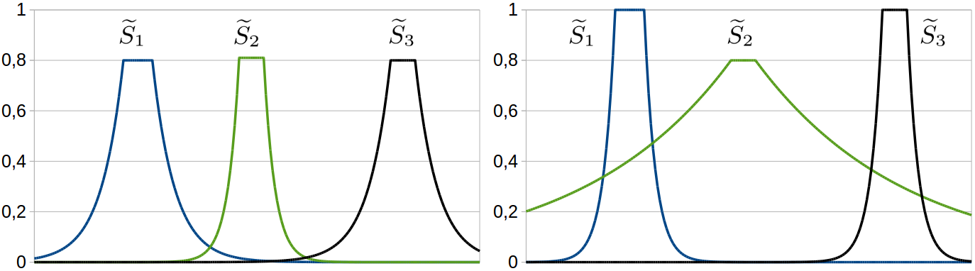
Figure 4: Two problematic cases for Bs​o​f​t​(S~1,S~2,S~3)B_{soft}(\widetilde{S}_{1},\widetilde{S}_{2},\widetilde{S}_{3}).

Unfortunately, this definition yields some unintutive results: If we consider the three concepts in Figure 4a, where μ0(1)=μ0(3)=0.80\mu_{0}^{(1)}=\mu_{0}^{(3)}=0.80 and μ0(2)=0.81\mu_{0}^{(2)}=0.81, then we get that Bs​o​f​t​(S~1,S~2,S~3)=0.0B_{soft}(\widetilde{S}_{1},\widetilde{S}_{2},\widetilde{S}_{3})=0.0, as for α=0.81\alpha=0.81, S~1α=S~3α=∅\widetilde{S}_{1}^{\alpha}=\widetilde{S}_{3}^{\alpha}=\emptyset. Also in the example shown in Figure 4b, we get Bs​o​f​t​(S~1,S~2,S~3)=0.0B_{soft}(\widetilde{S}_{1},\widetilde{S}_{2},\widetilde{S}_{3})=0.0: For α→0\alpha\rightarrow 0, S~2α\widetilde{S}_{2}^{\alpha} becomes much larger than S~1α\widetilde{S}_{1}^{\alpha} and S~3α\widetilde{S}_{3}^{\alpha} and we can select a point y∈S~2αy\in\widetilde{S}_{2}^{\alpha} for which Bs​o​f​t​(x,y,z)B_{soft}(x,y,z) becomes arbitrarily small independent of the choices for xx and zz.

In order to achieve a more generous degradation in cases like the ones depicted in Figure 4, we propose to aggregate over the α\alpha-cuts not by taking the minimum, but through an integration. As we integrate over α\alpha in the interval [0,1][0,1] and as the degree of betweenness computed for each α\alpha-cut also lies in the interval [0,1][0,1], the result of this integration is also a number between zero and one. We define:

Bs​o​f​ti​n​t​e​g​r​a​l​(S~1,S~2,S~3):=∫01miny∈S~2α⁡maxx∈S~1α​maxz∈S~3α​d⁡(x,z)d⁡(x,y)+d⁡(y,z)​𝑑αB_{soft}^{integral}(\widetilde{S}_{1},\widetilde{S}_{2},\widetilde{S}_{3}):=\int_{0}^{1}\min_{y\in\widetilde{S}_{2}^{\alpha}}\max_{x\in\widetilde{S}_{1}^{\alpha}}\max_{z\in\widetilde{S}_{3}^{\alpha}}\frac{d(x,z)}{d(x,y)+d(y,z)}\;d\alpha

All of the properties discovered above for Bs​o​f​t​(S~1,S~2,S~3)B_{soft}(\widetilde{S}_{1},\widetilde{S}_{2},\widetilde{S}_{3}) still hold for Bs​o​f​ti​n​t​e​g​r​a​l​(S~1,S~2,S~3)B_{soft}^{integral}(\widetilde{S}_{1},\widetilde{S}_{2},\widetilde{S}_{3}). However, in the examples from Figure 4 we do not get the unintuitive result of Bs​o​f​ti​n​t​e​g​r​a​l​(S~1,S~3,S~3)=0.0B_{soft}^{integral}(\widetilde{S}_{1},\widetilde{S}_{3},\widetilde{S}_{3})=0.0.

4 Illustrative Example

4.1 A Conceptual Space and its Concepts

We consider a very simplified conceptual space for fruits, consisting of the following domains and dimensions:

Δ={δc​o​l​o​r={dh​u​e},δs​h​a​p​e={dr​o​u​n​d},δt​a​s​t​e={ds​w​e​e​t}}\Delta=\left\{\delta_{color}=\left\{d_{hue}\right\},\delta_{shape}=\left\{d_{round}\right\},\delta_{taste}=\left\{d_{sweet}\right\}\right\}

dh​u​ed_{hue} describes the hue of the observation’s color, ranging from 0.000.00 (purple) to 1.001.00 (red). dr​o​u​n​dd_{round} measures the percentage to which the bounding circle of an object is filled. ds​w​e​e​td_{sweet} represents the relative amount of sugar contained in the fruit, ranging from 0.00 (no sugar) to 1.00 (high sugar content). As all domains are one-dimensional, the dimension weights wdw_{d} are always equal to 1.00 for all concepts. We assume that the dimensions are ordered like this: dh​u​e,dr​o​u​n​d,ds​w​e​e​td_{hue},d_{round},d_{sweet}. Table 1 defines several concepts in this space and Figure 5 visualizes them.

Table 1: Definitions of several concepts.
Concept ΔS\Delta_{S} p−p^{-} p+p^{+} μ0\mu_{0} cc WW
wδc​o​l​o​rw_{\delta_{color}} wδs​h​a​p​ew_{\delta_{shape}} wδt​a​s​t​ew_{\delta_{taste}}
Orange Δ\Delta (0.80, 0.90, 0.60) (0.90, 1.00, 0.70) 1.0 15.0 1.00 1.00 1.00
Lemon Δ\Delta (0.70, 0.45, 0.00) (0.80, 0.55, 0.10) 1.0 20.0 0.50 0.50 2.00
Granny Δ\Delta (0.55, 0.70, 0.35) (0.60, 0.80, 0.45) 1.0 25.0 1.00 1.00 1.00
Smith
Apple Δ\Delta (0.50, 0.65, 0.35) (0.80, 0.80, 0.50) 1.0 10.0 0.50 1.50 1.00
(0.65, 0.65, 0.40) (0.85, 0.80, 0.55)
(0.70, 0.65, 0.45) (1.00, 0.80, 0.60)
Red {δc​o​l​o​r}\{\delta_{color}\} (0.90, -∞\infty, -∞\infty) (1.00, +∞\infty, +∞\infty) 1.0 20.0 1.00 – –

Refer to caption
Figure 5: Top: Three-dimensional visualization of the fruit space (only cores). Bottom: Two-dimensional visualizations of the fruit space (cores and 0.5-cuts). The concepts are labeled as follows: red (1), apple (2), lemon (3), orange (4), Granny Smith (5).

4.2 Computations

Table 2: Computations of different relations. Note that S​u​b​(S~1,S~2)=I​m​p​l​(S~1,S~2)=S​i​mS​(S~1,S~2)Sub(\widetilde{S}_{1},\widetilde{S}_{2})=Impl(\widetilde{S}_{1},\widetilde{S}_{2})=Sim_{S}(\widetilde{S}_{1},\widetilde{S}_{2}).
S~1\widetilde{S}_{1} S~2\widetilde{S}_{2} M⁡(S~1)M(\widetilde{S}_{1}) M⁡(S~2)M(\widetilde{S}_{2}) S​u​b​(S~1,S~2)Sub(\widetilde{S}_{1},\widetilde{S}_{2}) S​u​b​(S~2,S~1)Sub(\widetilde{S}_{2},\widetilde{S}_{1}) S​i​mJ​(S~1,S~2)Sim_{J}(\widetilde{S}_{1},\widetilde{S}_{2}) S​i​mJ​(S~2,S~1)Sim_{J}(\widetilde{S}_{2},\widetilde{S}_{1})
Granny Smith Apple 0.0042 0.1048 1.0000 0.1171 0.2570 0.2570
Orange Apple 0.0127 0.1048 0.1800 0.0333 0.0414 0.0414
Lemon Apple 0.0135 0.1048 0.0422 0.0054 0.0073 0.0073
Red Apple 0.2000 0.1048 1.0000 0.3333 0.4286 0.4286
S~1\widetilde{S}_{1} S~2\widetilde{S}_{2} S~3\widetilde{S}_{3} Bs​o​f​t​(S~1,S~2,S~3)B_{soft}(\widetilde{S}_{1},\widetilde{S}_{2},\widetilde{S}_{3}) Bs​o​f​ti​n​t​e​g​r​a​l​(S~1,S~2,S~3)B_{soft}^{integral}(\widetilde{S}_{1},\widetilde{S}_{2},\widetilde{S}_{3})
Lemon Apple Orange 0.0000 0.8623
Lemon Granny Smith Orange 0.8254 0.9161
Granny Smith Apple Red 0.0000 0.0000
Apple Granny Smith Orange 1.0000 1.0000

Table 2 shows the results of using the definitions from Section 3 on the concepts defined in Section 4.1. Note that M⁡(S~l​e​m​o​n)≠M⁡(S~o​r​a​n​g​e)M(\widetilde{S}_{lemon})\neq M(\widetilde{S}_{orange}) because the two concepts have different weights and different sensitivity parameters. Also all relations involving the property “red” tend to yield relatively high numbers – this is because all computations only take place within the single domain on which “red” is defined. The numbers computed for the subsethood/implication relation nicely reflect our intuitive expectations. The numbers also nicely illustrate the difference between the asymmetric S​i​mSSim_{S} and the symmetric S​i​mJSim_{J} similarity functions. The values of S​i​mJ​(S~1,S~2)Sim_{J}(\widetilde{S}_{1},\widetilde{S}_{2}) are always between S​i​mS​(S~1,S~2)Sim_{S}(\widetilde{S}_{1},\widetilde{S}_{2}) and S​i​mS​(S~2,S~1)Sim_{S}(\widetilde{S}_{2},\widetilde{S}_{1}) while tending towards the smaller of the two numbers. Please note that for none of the examples we get a value for S​i​mJSim_{J} that is close to one. The numbers derived for the two betweenness relations show that Bs​o​f​ti​n​t​e​g​r​a​lB_{soft}^{integral} is always greater or equal than Bs​o​f​tB_{soft}. They agree on borderline cases: When computing the betweenness of concepts defined on different sets of domains (e.g., Granny Smith, apple, and red) they return zero, and when the middle concept is a subset of one of the outer concepts (e.e.g, apple, Granny Smith, and orange), they return one. The first example (lemon, apple, orange) shows the more generous degradation of Bs​o​f​ti​n​t​e​g​r​a​lB_{soft}^{integral} in a case similar to the one from Figure 4b.

5 Related Work

Our work is of course not the first attempt to devise an implementable formalization of the conceptual spaces framework.

An early formalization was done by [Aisbett and Gibbon, 2001]. Like we, they consider concepts to be regions in the overall conceptual space. However, they stick with the assumption of convexity and do not define concepts in a parametric way. The only operations they provide are distance and similarity of points and regions. Their formalization targets the interplay of symbols and geometric representations, but it is too abstract to be implementable.

[Rickard, 2006] provides a formalization based on fuzziness. He represents concepts as co-occurence matrices of their properties. By using some mathematical transformations, he interprets these matrices as fuzzy sets on the universe of ordered property pairs. Operations defined on these concepts include similarity judgements between concepts and between concepts and instances. Rickard’s representation of correlations is not geometrical: He first discretizes the domains (by defining properties) and then computes the co-occurences between these properties. Depending on the discretization, this might lead to a relatively coarse-grained notion of correlation. Moreover, as properties and concepts are represented in different ways, one has to use different learning and reasoning mechanisms for them. His formalization is also not easy to work with due to the complex mathematical transformations involved.

[Adams and Raubal, 2009a] represent concepts by one convex polytope per domain. This allows for efficient computations while being potentially more expressive than our cuboid-based approach. The Manhattan metric is used to combine different domains. However, correlations between different domains are not taken into account and cannot be expressed in this formalization as each convex polytope is only defined on a single domain. Adams and Raubal also define operations on concepts, namely intersection, similarity computation, and concept combination. This makes their formalization quite similar in spirit to ours.

[Lewis and Lawry, 2016] formalize conceptual spaces using random set theory. They define properties as random sets within single domains and concepts as random sets in a boolean space whose dimensions indicate the presence or absence of properties. In order to define this boolean space, a single property is taken from each domain. Their approach is similar to ours in using a distance-based membership function to a set of prototypical points. However, their work purely focuses on modeling conjunctive concept combinations and does not consider correlations between domains.

As one can see, none of the formalizations listed above provides a set of operations that is as comprehensive as the one offered by our extended formalization.

6 Conclusion and Future Work

In this paper, we extended our previous formalization of the conceptual spaces framework by providing ways to measure relations between concepts: concept size, subsethood, implication, similarity, and betweenness. This considerably extends our framework’s capabilities for representing knowledge and makes it (to the best of our knowledge) the most thorough and comprehensive formalization of conceptual spaces developed so far. A python implementation of our formalization is publicly available on GitHub under https://www.github.com/lbechberger/ConceptualSpaces [Bechberger, 2018].

Our overall research goal is to use machine learning in conceptual spaces. Therefore, our future work will focus on putting this formalization to practical use in a machine learning context.

References

  • [Adams and Raubal, 2009a] Adams, B. and Raubal, M. (2009a). A Metric Conceptual Space Algebra. In 9th International Conference on Spatial Information Theory, pages 51–68. Springer Berlin Heidelberg.
  • [Adams and Raubal, 2009b] Adams, B. and Raubal, M. (2009b). Conceptual Space Markup Language (CSML): Towards the Cognitive Semantic Web. 2009 IEEE International Conference on Semantic Computing.
  • [Aggarwal et al., 2001] Aggarwal, C. C., Hinneburg, A., and Keim, D. A. (2001). On the Surprising Behavior of Distance Metrics in High Dimensional Space. In 8th International Conference on Database Theory, pages 420–434. Springer Berlin Heidelberg.
  • [Aisbett and Gibbon, 2001] Aisbett, J. and Gibbon, G. (2001). A General Formulation of Conceptual Spaces as a Meso Level Representation. Artificial Intelligence, 133(1-2):189–232.
  • [Attneave, 1950] Attneave, F. (1950). Dimensions of Similarity. The American Journal of Psychology, 63(4):516–556.
  • [Bechberger, 2018] Bechberger, L. (2018). lbechberger/ConceptualSpaces: Version 1.2.0. https://doi.org/10.5281/zenodo.1200230.
  • [Bechberger and Kühnberger, 2017a] Bechberger, L. and Kühnberger, K.-U. (2017a). A Thorough Formalization of Conceptual Spaces. In Kern-Isberner, G., Fürnkranz, J., and Thimm, M., editors, KI 2017: Advances in Artificial Intelligence: 40th Annual German Conference on AI, Dortmund, Germany, September 25–29, 2017, Proceedings, pages 58–71. Springer International Publishing.
  • [Bechberger and Kühnberger, 2017b] Bechberger, L. and Kühnberger, K.-U. (2017b). Measuring Relations Between Concepts In Conceptual Spaces. In Bramer, M. and Petridis, M., editors, Artificial Intelligence XXXIV: 37th SGAI International Conference on Artificial Intelligence, AI 2017, Cambridge, UK, December 12-14, 2017, Proceedings, pages 87–100. Springer International Publishing.
  • [Bělohlávek and Klir, 2011] Bělohlávek, R. and Klir, G. J. (2011). Concepts and Fuzzy Logic. MIT Press.
  • [Billman and Knutson, 1996] Billman, D. and Knutson, J. (1996). Unsupervised Concept Learning and Value Systematicitiy: A Complex Whole Aids Learning the Parts. Journal of Experimental Psychology: Learning, Memory, and Cognition, 22(2):458–475.
  • [Bogart, 1989] Bogart, K. P. (1989). Introductory Combinatorics. Saunders College Publishing, Philadelphia, PA, USA, 2nd edition.
  • [Bouchon-Meunier et al., 1996] Bouchon-Meunier, B., Rifqi, M., and Bothorel, S. (1996). Towards General Measures of Comparison of Objects. Fuzzy Sets and Systems, 84(2):143–153.
  • [Chella et al., 2003] Chella, A., Frixione, M., and Gaglio, S. (2003). Anchoring Symbols to Conceptual Spaces: The Case of Dynamic Scenarios. Robotics and Autonomous Systems, 43(2-3):175–188.
  • [DeRise, 1992] DeRise, G. (1992). Some n-Dimensional Geometry. International Journal of Mathematical Education in Science and Technology, 23(3):371–379.
  • [Derrac and Schockaert, 2014] Derrac, J. and Schockaert, S. (2014). Enriching Taxonomies of Place Types Using Flickr. In Beierle, C. and Meghini, C., editors, Foundations of Information and Knowledge Systems: 8th International Symposium, FoIKS 2014, pages 174–192, Cham. Springer International Publishing.
  • [Derrac and Schockaert, 2015] Derrac, J. and Schockaert, S. (2015). Inducing Semantic Relations from Conceptual Spaces: A Data-Driven Approach to Plausible Reasoning. Artificial Intelligence, 228:66–94.
  • [Douven et al., 2011] Douven, I., Decock, L., Dietz, R., and Égré, P. (2011). Vagueness: A Conceptual Spaces Approach. Journal of Philosophical Logic, 42(1):137–160.
  • [Fiorini et al., 2013] Fiorini, S. R., Gärdenfors, P., and Abel, M. (2013). Representing Part-Whole Relations in Conceptual Spaces. Cognitive Processing, 15(2):127–142.
  • [Gärdenfors, 2000] Gärdenfors, P. (2000). Conceptual Spaces: The Geometry of Thought. MIT press.
  • [Gärdenfors, 2014] Gärdenfors, P. (2014). The Geometry of Meaning: Semantics Based on Conceptual Spaces. MIT Press.
  • [Harnad, 1990] Harnad, S. (1990). The Symbol Grounding Problem. Physica D: Nonlinear Phenomena, 42(1-3):335–346.
  • [Johannesson, 2001] Johannesson, M. (2001). The Problem of Combining Integral and Separable Dimensions. Technical Report HS-IDA-TR-01-002, University of Skövde, School of Humanities and Informatics.
  • [Kosko, 1992] Kosko, B. (1992). Neural Networks and Fuzzy Systems: A Dynamical Systems Approach to Machine Intelligence. Prentice Hall.
  • [Lewis and Lawry, 2016] Lewis, M. and Lawry, J. (2016). Hierarchical Conceptual Spaces for Concept Combination. Artificial Intelligence, 237:204–227.
  • [Lieto et al., 2017] Lieto, A., Radicioni, D. P., and Rho, V. (2017). Dual PECCS: a cognitive system for conceptual representation and categorization. Journal of Experimental & Theoretical Artificial Intelligence, 29(2):433–452.
  • [Mas et al., 2007] Mas, M., Monserrat, M., Torrens, J., and Trillas, E. (2007). A Survey on Fuzzy Implication Functions. IEEE Transactions on Fuzzy Systems, 15(6):1107–1121.
  • [Murphy, 2002] Murphy, G. (2002). The Big Book of Concepts. MIT Press.
  • [Rickard, 2006] Rickard, J. T. (2006). A Concept Geometry for Conceptual Spaces. Fuzzy Optimization and Decision Making, 5(4):311–329.
  • [Schockaert and Prade, 2011] Schockaert, S. and Prade, H. (2011). Qualitative Reasoning about Incomplete Categorization Rules Based on Interpolation and Extrapolation in Conceptual Spaces, pages 303–316. Springer Berlin Heidelberg, Berlin, Heidelberg.
  • [Shepard, 1964] Shepard, R. N. (1964). Attention and the Metric Structure of the Stimulus Space. Journal of Mathematical Psychology, 1(1):54–87.
  • [Silvester, 2000] Silvester, J. R. (2000). Determinants of Block Matrices. The Mathematical Gazette, 84(501):460–467.
  • [Smith, 1968] Smith, C. R. (1968). A Characterization of Star-Shaped Sets. The American Mathematical Monthly, 75(4):386.
  • [Tversky, 1977] Tversky, A. (1977). Features of Similarity. Psychological Review, 84(4):327.
  • [Zadeh, 1965] Zadeh, L. A. (1965). Fuzzy Sets. Information and Control, 8(3):338–353.
  • [Zadeh, 1975] Zadeh, L. A. (1975). The Concept of a Linguistic Variable and its Application to Approximate Reasoning. Information Sciences, 8(3):199–249.

Appendix 0.A Concept Size

0.A.1 Hyperballs under the Unweighted Metric

In general, a hyperball of radius rr around a point pp can be defined as the set of all points with a distance of at most rr to pp:

H={x∈C​S|d⁡(x,p)≤r}H=\{x\in CS\;|\;d(x,p)\leq r\}
Refer to caption
Figure 6: Left: Two-dimensional hyperball under the Euclidean metric. Middle: Two-dimensional hyperball under the Manhattan metric. Right: Three-dimensional hyperball under the combined metric (with domain structure Δ={δ1={d1,d2},δ2={d3}}\Delta=\{\delta_{1}=\{d_{1},d_{2}\},\delta_{2}=\{d_{3}\}\}).

If the Euclidean distance dEd_{E} is used, this corresponds to our intuitive notion of a ball – a round shape centered at pp. However, under the Manhattan distance dMd_{M}, hyperballs have the shape of diamonds. Under the combined distance dCΔd_{C}^{\Delta}, a hyperball in three dimensions has the shape of a double cone (cf. Figure 6).

As similarity is inversely related to distance, one can interpret a hyperball in a conceptual space as the set of all points that have a minimal similarity α\alpha to the central point pp, where α\alpha depends on the radius of the hyperball.

In this section, we assume an unweighted version of dCΔd_{C}^{\Delta}:

dCΔ​(x,y)=∑δ∈Δ∑d∈δ|xd−yd|2d_{C}^{\Delta}(x,y)=\sum_{\delta\in\Delta}\sqrt{\sum_{d\in\delta}|x_{d}-y_{d}|^{2}}

In order to derive a formula for the hypervolume of a hyperball under dCΔd_{C}^{\Delta}, we need to use the following three lemmata:

Lemma 2
∫02​π∫0π∫0π…​∫0πsinn−2⁡(ϕ1)​sinn−3⁡(ϕ2)​…​sin⁡(ϕn−2)​d​ϕ1​…​d​ϕn−1=2⋅πn2Γ⁡(n2)\int_{0}^{2\pi}\int_{0}^{\pi}\int_{0}^{\pi}\dots\int_{0}^{\pi}\sin^{n-2}(\phi_{1})\sin^{n-3}(\phi_{2})\dots\sin(\phi_{n-2})d\phi_{1}\dots d\phi_{n-1}=2\cdot\frac{\pi^{\frac{n}{2}}}{\Gamma\left(\frac{n}{2}\right)}

where Γ⁡(⋅)\Gamma(\cdot) is Euler’s Gamma function and n∈ℕn\in\mathbb{N}.

Proof
I\displaystyle I =∫02​π∫0π∫0π…​∫0πsinn−2⁡(ϕ1)​sinn−3⁡(ϕ2)​…​sin⁡(ϕn−2)​d​ϕ1​…​d​ϕn−1\displaystyle=\int_{0}^{2\pi}\int_{0}^{\pi}\int_{0}^{\pi}\dots\int_{0}^{\pi}\sin^{n-2}(\phi_{1})\sin^{n-3}(\phi_{2})\dots\sin(\phi_{n-2})d\phi_{1}\dots d\phi_{n-1}
=(∫02​π1dϕn−1)(∫0πsin(ϕn−2)dϕn−2)⋯(∫0πsinn−2(ϕ1)dϕ1)\displaystyle=\left(\int\displaylimits_{0}^{2\pi}1\;d\phi_{n-1}\right)\left(\int\displaylimits_{0}^{\pi}\sin(\phi_{n-2})\;d\phi_{n-2}\right)\cdots\left(\int\displaylimits_{0}^{\pi}\sin^{n-2}(\phi_{1})\;d\phi_{1}\right)
=(4⋅∫0π21dϕn−1)(2⋅∫0π2sin(ϕn−2)dϕn−2)⋯(2⋅∫0π2sinn−2(ϕ1)dϕ1)\displaystyle=\left(4\cdot\int\displaylimits_{0}^{\frac{\pi}{2}}1\;d\phi_{n-1}\right)\left(2\cdot\int\displaylimits_{0}^{\frac{\pi}{2}}\sin(\phi_{n-2})\;d\phi_{n-2}\right)\cdots\left(2\cdot\int\displaylimits_{0}^{\frac{\pi}{2}}\sin^{n-2}(\phi_{1})\;d\phi_{1}\right)

We can now use the definition of the Beta function, which is

B⁡(x,y)=2⋅∫0π2sin2​x−1⁡(ϕ)​cos2​y−1⁡(ϕ)​𝑑ϕB(x,y)=2\cdot\int\displaylimits_{0}^{\frac{\pi}{2}}\sin^{2x-1}(\phi)\cos^{2y-1}(\phi)\;d\phi

Using y=12y=\frac{1}{2}, we get:

I\displaystyle I =(4⋅∫0π21dϕn−1)(2⋅∫0π2sin(ϕn−2)dϕn−2)⋯(2⋅∫0π2sinn−2(ϕ1)dϕ1)\displaystyle=\left(4\cdot\int\displaylimits_{0}^{\frac{\pi}{2}}1\;d\phi_{n-1}\right)\left(2\cdot\int\displaylimits_{0}^{\frac{\pi}{2}}\sin(\phi_{n-2})\;d\phi_{n-2}\right)\cdots\left(2\cdot\int\displaylimits_{0}^{\frac{\pi}{2}}\sin^{n-2}(\phi_{1})\;d\phi_{1}\right)
=2⋅B(12,12)⋅B(1,12)⋯B(n−22,12)⋅B(n−12,12)\displaystyle=2\cdot B\left(\frac{1}{2},\frac{1}{2}\right)\cdot B\left(1,\frac{1}{2}\right)\cdots B\left(\frac{n-2}{2},\frac{1}{2}\right)\cdot B\left(\frac{n-1}{2},\frac{1}{2}\right)

Next, we use the identity B⁡(x,y)=Γ⁡(x)​Γ​(y)Γ⁡(x+y)B(x,y)=\frac{\Gamma(x)\Gamma(y)}{\Gamma(x+y)} with Euler’s Gamma function Γ\Gamma and the fact that Γ⁡(12)=π\Gamma(\frac{1}{2})=\sqrt{\pi}. We get:

I=2⋅Γ⁡(12)​Γ​(12)Γ⁡(1)⋅Γ⁡(1)​Γ​(12)Γ⁡(32)⋯Γ⁡(n−22)​Γ​(12)Γ⁡(n−12)⋅Γ⁡(n−12)​Γ​(12)Γ⁡(n2)=2⋅Γ​(12)nΓ⁡(n2)=2⋅πn2Γ⁡(n2)I=2\cdot\frac{\Gamma(\frac{1}{2})\Gamma(\frac{1}{2})}{\Gamma(1)}\cdot\frac{\Gamma(1)\Gamma(\frac{1}{2})}{\Gamma(\frac{3}{2})}\cdots\frac{\Gamma(\frac{n-2}{2})\Gamma(\frac{1}{2})}{\Gamma(\frac{n-1}{2})}\cdot\frac{\Gamma(\frac{n-1}{2})\Gamma(\frac{1}{2})}{\Gamma(\frac{n}{2})}=2\cdot\frac{\Gamma(\frac{1}{2})^{n}}{\Gamma(\frac{n}{2})}=2\cdot\frac{\pi^{\frac{n}{2}}}{\Gamma(\frac{n}{2})}

∎

Lemma 3

For any natural number j>0j>0 and any a,b∈ℝa,b\in\mathbb{R}, the following equation holds:

∫0r−∑i=1j−1rirja−1⋅(r−∑i=1jri)b​d​rj=B⁡(a,b+1)⋅(r−∑i=1j−1ri)a+b\int_{0}^{r-\sum_{i=1}^{j-1}r_{i}}r_{j}^{a-1}\cdot\left(r-\sum_{i=1}^{j}r_{i}\right)^{b}dr_{j}=B(a,b+1)\cdot\left(r-\sum_{i=1}^{j-1}r_{i}\right)^{a+b}
Proof

We can make a variable change by defining rj=(r−∑i=1j−1ri)⋅zr_{j}=\left(r-\sum_{i=1}^{j-1}r_{i}\right)\cdot z which gives d​rj=(r−∑i=1j−1ri)⋅d​zdr_{j}=\left(r-\sum_{i=1}^{j-1}r_{i}\right)\cdot dz. This results in:

∫0r−∑i=1j−1rirja−1⋅(r−∑i=1jri)b​d​rj\displaystyle\int_{0}^{r-\sum_{i=1}^{j-1}r_{i}}r_{j}^{a-1}\cdot\left(r-\sum_{i=1}^{j}r_{i}\right)^{b}dr_{j}
=∫01(r−∑i=1j−1ri)a−1⋅za−1⋅(r−∑i=1j−1ri−(r−∑i=1j−1ri)⋅z)b⋅(r−∑i=1j−1ri)​𝑑z\displaystyle=\int_{0}^{1}\left(r-\sum_{i=1}^{j-1}r_{i}\right)^{a-1}\cdot z^{a-1}\cdot\left(r-\sum_{i=1}^{j-1}r_{i}-\left(r-\sum_{i=1}^{j-1}r_{i}\right)\cdot z\right)^{b}\cdot\left(r-\sum_{i=1}^{j-1}r_{i}\right)dz
=(r−∑i=1j−1ri)a−1+b+1​∫01za−1​(1−z)b​𝑑z=(r−∑i=1j−1ri)a+b⋅B⁡(a,b+1)\displaystyle=\left(r-\sum_{i=1}^{j-1}r_{i}\right)^{a-1+b+1}\int_{0}^{1}z^{a-1}(1-z)^{b}dz=\left(r-\sum_{i=1}^{j-1}r_{i}\right)^{a+b}\cdot B(a,b+1)

The last transformation uses the fact that B⁡(x,y)=∫01tx−1​(1−t)y−1​𝑑tB(x,y)=\int_{0}^{1}t^{x-1}(1-t)^{y-1}dt. ∎

Lemma 4

For any natural number k>0k>0, any r1,…,rk,n1,…,nk>0r_{1},\dots,r_{k},n_{1},\dots,n_{k}>0, n=∑i=0knin=\sum_{i=0}^{k}n_{i}, r=∑i=0krir=\sum_{i=0}^{k}r_{i}, the following equation holds:

∫0rr1n1−1​∫0r−r1r2n2−1​…​∫0r−∑i=1k−1rirknk−1​d​rk​…​d​r1=rnΓ⁡(n+1)​∏i=1kΓ⁡(ni)\int_{0}^{r}r_{1}^{n_{1}-1}\int_{0}^{r-r_{1}}r_{2}^{n_{2}-1}\dots\int_{0}^{r-\sum_{i=1}^{k-1}r_{i}}r_{k}^{n_{k}-1}dr_{k}\dots dr_{1}=\frac{r^{n}}{\Gamma(n+1)}\prod_{i=1}^{k}\Gamma(n_{i})
Proof

Using Lemma 3, we can solve the innermost integral by setting j=k,a=nk,b=0j=k,a=n_{k},b=0, which gives us B⁡(nk,1)⋅(r−∑i=1k−1ri)nkB(n_{k},1)\cdot\left(r-\sum_{i=1}^{k-1}r_{i}\right)^{n_{k}}. Therefore:

I\displaystyle I =∫0rr1n1−1​∫0r−r1r2n2−1​…​∫0r−∑i=1k−1rirknk−1​d​rk​…​d​r1\displaystyle=\int_{0}^{r}r_{1}^{n_{1}-1}\int_{0}^{r-r_{1}}r_{2}^{n_{2}-1}\dots\int_{0}^{r-\sum_{i=1}^{k-1}r_{i}}r_{k}^{n_{k}-1}dr_{k}\dots dr_{1}
=B⁡(nk,1)⋅∫0rr1n1−1​…​∫0r−∑i=1k−2rirk−1nk−1−1⋅(r−∑i=1k−1ri)nk​d​rk−1​…​d​r1\displaystyle=B(n_{k},1)\cdot\int_{0}^{r}r_{1}^{n_{1}-1}\dots\int_{0}^{r-\sum_{i=1}^{k-2}r_{i}}r_{k-1}^{n_{k-1}-1}\cdot\left(r-\sum_{i=1}^{k-1}r_{i}\right)^{n_{k}}dr_{k-1}\dots dr_{1}

As one can see, we can again apply Lemma 3 to the innermost integral. Repeatedly applying Lemma 3 finally results in:

I=B⁡(nk,1)⋅B⁡(nk−1,nk+1)⋅⋯⋅B⁡(n1,n2+⋯+nk+1)⋅rn1+⋯+nkI=B(n_{k},1)\cdot B(n_{k-1},n_{k}+1)\cdot\dots\cdot B(n_{1},n_{2}+\dots+n_{k}+1)\cdot r^{n_{1}+\dots+n_{k}}

We use that B⁡(x,y)=Γ⁡(x)​Γ​(y)Γ⁡(x+y)B(x,y)=\frac{\Gamma(x)\Gamma(y)}{\Gamma(x+y)} in order to rewrite this equation:

I=rn1+⋯+nk⋅Γ⁡(nk)​Γ​(1)Γ⁡(nk+1)⋅Γ⁡(nk−1)​Γ​(nk+1)Γ⁡(nk−1+nk+1)⋯Γ⁡(n1)​Γ​(n2+⋯+nk+1)Γ⁡(n1+n2+⋯+nk+1)I=r^{n_{1}+\dots+n_{k}}\cdot\frac{\Gamma(n_{k})\Gamma(1)}{\Gamma(n_{k}+1)}\cdot\frac{\Gamma(n_{k-1})\Gamma(n_{k}+1)}{\Gamma(n_{k-1}+n_{k}+1)}\cdots\frac{\Gamma(n_{1})\Gamma(n_{2}+\dots+n_{k}+1)}{\Gamma(n_{1}+n_{2}+\dots+n_{k}+1)}

Because Γ⁡(1)=1\Gamma(1)=1 and because most of the terms cancel out, this reduces to:

I=rn1+⋯+nk⋅Γ(nk)⋯Γ(n1)⋅1Γ⁡(n1+⋯+nk+1)=rnΓ⁡(n+1)∏i=1kΓ(ni)I=r^{n_{1}+\dots+n_{k}}\cdot\Gamma(n_{k})\cdots\Gamma(n_{1})\cdot\frac{1}{\Gamma(n_{1}+\dots+n_{k}+1)}=\frac{r^{n}}{\Gamma(n+1)}\prod_{i=1}^{k}\Gamma(n_{i})

∎

Using these three lemata, we can now derive the size of a hyperball in a conceptual space without domain and dimension weights:

Lemma 5

The hypervolume of a hyperball with radius rr in a space with the unweighted combined metric dCΔd_{C}^{\Delta} and the domain structure Δ\Delta can be computed in the following way, where nn is the overall number of dimensions and nδn_{\delta} is the number of dimensions in domain δ\delta:

V⁡(r,Δ)=rnn!​∏δ∈Δ(nδ!​πnδ2Γ⁡(nδ2+1))V(r,\Delta)=\frac{r^{n}}{n!}\prod_{\delta\in\Delta}\left(n_{\delta}!\frac{\pi^{\frac{n_{\delta}}{2}}}{\Gamma\left(\frac{n_{\delta}}{2}+1\right)}\right)
Proof

The hyperball can be defined as the set of all points that have a distance of maximally rr to the origin, i.e.,

H={x∈C​S|dCΔ​(x,0)=∑δ∈Δ∑d∈δxd2≤r}H=\Big\{x\in CS\;|\;d_{C}^{\Delta}(x,0)=\sum_{\delta\in\Delta}\sqrt{\sum_{d\in\delta}x_{d}^{2}}\leq r\Big\}

If we define ∀δ∈Δ:rδ:=∑d∈δxd2\forall\delta\in\Delta:r_{\delta}:=\sqrt{\sum_{d\in\delta}x_{d}^{2}}, we can easily see that ∑δ∈Δrδ≤r\sum_{\delta\in\Delta}r_{\delta}\leq r. The term rδr_{\delta} can be interpreted as the distance between xx and the origin within the domain δ\delta. The constraint ∑δ∈Δrδ≤r\sum_{\delta\in\Delta}r_{\delta}\leq r then simply means that the sum of domain-wise distances is less than the given radius. One can thus interpret rδr_{\delta} as the radius within domain δ\delta.

We would ultimately like to compute

V⁡(r,Δ)=∫…​∫H1​𝑑HV(r,\Delta)=\int\dots\int_{H}1\;dH

This integration becomes much easier if we use spherical coordinates instead of the Cartesian coordinates provided by our conceptual space.

Let us first consider the case of a single domain δ\delta of size nδn_{\delta}. A single domain corresponds to a standard Euclidean space, therefore we can use the standard procedure of changing to spherical coordinates (cf., e.g., [DeRise, 1992]). Let us index the dimensions of δ\delta as d1,…,dnδd_{1},\dots,d_{n_{\delta}}. The coordinate change within the domain δ\delta then looks like this:

x1\displaystyle x_{1} =t⋅cos⁡(ϕ1)\displaystyle=t\cdot\cos(\phi_{1})
x2\displaystyle x_{2} =t⋅sin⁡(ϕ1)⋅cos⁡(ϕ2)\displaystyle=t\cdot\sin(\phi_{1})\cdot\cos(\phi_{2})
⋮\displaystyle\hskip 5.69046pt\vdots
xnδ−1\displaystyle x_{{n_{\delta}}-1} =t⋅sin(ϕ1)⋯sin(ϕnδ−2)⋅cos(ϕnδ−1)\displaystyle=t\cdot\sin(\phi_{1})\cdots\sin(\phi_{{n_{\delta}}-2})\cdot\cos(\phi_{{n_{\delta}}-1})
xnδ\displaystyle x_{{n_{\delta}}} =t⋅sin(ϕ1)⋯sin(ϕnδ−2)⋅sin(ϕnδ−1)\displaystyle=t\cdot\sin(\phi_{1})\cdots\sin(\phi_{{n_{\delta}}-2})\cdot\sin(\phi_{{n_{\delta}}-1})

In order to switch the integral to spherical coordinates, we need to calucalate the volume element. This can be found by looking at the determinant of the transformation’s Jacobian matrix. The Jacobian matrix of the transformation of a single domain δ\delta can be written as follows:

Jδ=[δ​x1δ​tδ​x1δ​ϕ1…δ​x1δ​ϕnδ−1δ​x2δ​tδ​x2δ​ϕ1…δ​x2δ​ϕnδ−1⋮⋮⋱⋮δ​xnδδ​tδ​xnδδ​ϕ1…δ​xnδδ​ϕnδ−1]=\displaystyle J_{\delta}=\left[{\begin{array}[]{cccc}\frac{\delta x_{1}}{\delta t}&\frac{\delta x_{1}}{\delta\phi_{1}}&\dots&\frac{\delta x_{1}}{\delta\phi_{{n_{\delta}}-1}}\\ \frac{\delta x_{2}}{\delta t}&\frac{\delta x_{2}}{\delta\phi_{1}}&\dots&\frac{\delta x_{2}}{\delta\phi_{{n_{\delta}}-1}}\\ \vdots&\vdots&\ddots&\vdots\\ \frac{\delta x_{{n_{\delta}}}}{\delta t}&\frac{\delta x_{{n_{\delta}}}}{\delta\phi_{1}}&\dots&\frac{\delta x_{{n_{\delta}}}}{\delta\phi_{{n_{\delta}}-1}}\\ \end{array}}\right]=
[cos⁡(ϕ1)−t​sin⁡(ϕ1)00…0sin⁡(ϕ1)​cos⁡(ϕ2)t​cos⁡(ϕ1)​cos⁡(ϕ2)−t​sin⁡(ϕ1)​sin⁡(ϕ2)0…0⋮⋮⋮⋮⋮⋮sin(ϕ1)⋯sin(ϕnδ−2)cos(ϕnδ−1)…………−tsin(ϕ1)⋯sin(ϕnδ−2)sin(ϕnδ−1)sin(ϕ1)⋯sin(ϕnδ−2)sin(ϕnδ−1)…………tsin(ϕ1)⋯sin(ϕnδ−2)cos(ϕnδ−1)]\displaystyle\hskip-5.69046pt\left[{\tiny\begin{array}[]{cccccc}\cos(\phi_{1})&-t\sin(\phi_{1})&0&0&\dots&0\\ \sin(\phi_{1})\cos(\phi_{2})&t\cos(\phi_{1})\cos(\phi_{2})&-t\sin(\phi_{1})\sin(\phi_{2})&0&\dots&0\\ \vdots&\vdots&\vdots&\vdots&\vdots&\vdots\\ \sin(\phi_{1})\cdots\sin(\phi_{{n_{\delta}}-2})\cos(\phi_{{n_{\delta}}-1})&\dots&\dots&\dots&\dots&-t\sin(\phi_{1})\cdots\sin(\phi_{{n_{\delta}}-2})\sin(\phi_{{n_{\delta}}-1})\\ \sin(\phi_{1})\cdots\sin(\phi_{{n_{\delta}}-2})\sin(\phi_{{n_{\delta}}-1})&\dots&\dots&\dots&\dots&t\sin(\phi_{1})\cdots\sin(\phi_{{n_{\delta}}-2})\cos(\phi_{{n_{\delta}}-1})\end{array}}\right]

The determinant of this matrix can be computed like this:

det(Jδ)=tnδ−1⋅sinnδ−2(ϕ1)⋅sinnδ−3(ϕ2)⋯sin(ϕnδ−2)det(J_{\delta})=t^{{n_{\delta}}-1}\cdot\sin^{{n_{\delta}}-2}(\phi_{1})\cdot\sin^{{n_{\delta}}-3}(\phi_{2})\cdots\sin(\phi_{{n_{\delta}}-2})

We can now perform the overall switch from Cartesian to spherical coordinates by performing this coordinate change for each domain individually. Let us index the Cartesian coordinates of a point xx in domain δ\delta by xδ,1,…,xδ,nδx_{\delta,1},\dots,x_{\delta,n_{\delta}}. Let us further index the spherical coordinates of domain δ\delta by rδr_{\delta} and ϕδ,1,…,ϕδ,nδ−1\phi_{\delta,1},\dots,\phi_{\delta,n_{\delta}-1}. Let k=|Δ|k=|\Delta| denote the total number of domains.

Because xδ,jx_{\delta,j} is defined independently from rδ′r_{\delta^{\prime}} and ϕδ′,j′\phi_{\delta^{\prime},j^{\prime}} for different domains δ≠δ′\delta\neq\delta^{\prime}, any derivative xδ,jrδ′\frac{x_{\delta,j}}{r_{\delta^{\prime}}} or xδ,jϕδ′,j′\frac{x_{\delta,j}}{\phi_{\delta^{\prime},j^{\prime}}} will be zero. If we apply the coordinate change to all domains at once, the Jacobian matrix of the overall transformation has therefore the structure of a block matrix:

J=[J10…00J2…0⋮⋮⋱⋮00…Jk]J=\left[{\begin{array}[]{cccc}J_{1}&0&\dots&0\\ 0&J_{2}&\dots&0\\ \vdots&\vdots&\ddots&\vdots\\ 0&0&\dots&J_{k}\\ \end{array}}\right]

The blocks on the diagonal are the Jacobian matrices of the individual domains as defined above, and all other blocks are filled with zeroes because all cross-domain derivatives are zero. Because the overall JJ is a block matrix, we get that d​e​t​(J)=∏δ∈Δd​e​t​(Jδ)det(J)=\prod_{\delta\in\Delta}det(J_{\delta}) (cf. [Silvester, 2000]). Our overall volume element is thus

det(J)=∏δ∈Δdet(Jδ)=∏δ∈Δrδnδ−1sinnδ−2(ϕδ,1)sinnδ−3(ϕδ,2)⋯sin(ϕδ,nδ−2)det(J)=\prod_{\delta\in\Delta}det(J_{\delta})=\prod_{\delta\in\Delta}r_{\delta}^{n_{\delta}-1}\sin^{n_{\delta}-2}(\phi_{\delta,1})\sin^{n_{\delta}-3}(\phi_{\delta,2})\cdots\sin(\phi_{\delta,n_{\delta}-2})

The limits of the angle integrals are [0,2​π][0,2\pi] for the outermost and [0,π][0,\pi] for all other integrals. Based on our constraint ∑δ∈Δrδ≤r\sum_{\delta\in\Delta}r_{\delta}\leq r, we can derive the limits for the integrals over the rδr_{\delta} as follows, assuming an arbitrarily ordered indexing δ1,…,δk\delta_{1},\dots,\delta_{k} of the domains:

r1\displaystyle r_{1} ∈[0,r]\displaystyle\in[0,r]
r2\displaystyle r_{2} ∈[0,r−r1]\displaystyle\in[0,r-r_{1}]
r3\displaystyle r_{3} ∈[0,r−r1−r2]\displaystyle\in[0,r-r_{1}-r_{2}]
⋮\displaystyle\hskip 5.69046pt\vdots
rk\displaystyle r_{k} ∈[0,r−∑i=1k−1ri]\displaystyle\in[0,r-\sum_{i=1}^{k-1}r_{i}]

The overall coordinate change therefore looks like this:

V\displaystyle V (r,Δ)=∫…​∫H1​𝑑H\displaystyle(r,\Delta)=\int\dots\int_{H}1\;dH
=∫ϕ1,n1−1=02​π∫ϕ1,n1−2=0π⋯∫ϕ1,1=0π∫r1=0r⏟δ=1⋯∫ϕk,nk−1=02​π∫ϕk,nk−2=0π⋯∫ϕk,1=0π∫rk=0r−∑i=1k−1ri⏟δ=k\displaystyle=\underbrace{\int\displaylimits_{\phi_{1,n_{1}-1}=0}^{2\pi}\int\displaylimits_{\phi_{1,n_{1}-2}=0}^{\pi}\cdots\int\displaylimits_{\phi_{1,1}=0}^{\pi}\int\displaylimits_{r_{1}=0}^{r}}_{\delta=1}\cdots\underbrace{\int\displaylimits_{\phi_{k,n_{k}-1}=0}^{2\pi}\int\displaylimits_{\phi_{k,n_{k}-2}=0}^{\pi}\cdots\int\displaylimits_{\phi_{k,1}=0}^{\pi}\int\displaylimits_{r_{k}=0}^{r-\sum_{i=1}^{k-1}r_{i}}}_{\delta=k}
r1n1−1sinn1−2(ϕ1,1)⋯sin(ϕ1,n1−2)⏟δ=1⋯rknk−1sinnk−2(ϕk,1)⋯sin(ϕk,nk−2)⏟δ=k\displaystyle\hskip 22.76228pt\underbrace{r_{1}^{n_{1}-1}\sin^{n_{1}-2}(\phi_{1,1})\cdots\sin(\phi_{1,n_{1}-2})}_{\delta=1}\cdots\underbrace{r_{k}^{n_{k}-1}\sin^{n_{k}-2}(\phi_{k,1})\cdots\sin(\phi_{k,n_{k}-2})}_{\delta=k}
d​rk​d​ϕk,1​…​d​ϕk,nk−1⏟δ=k​…​d​r1​d​ϕ1,1​…​d​ϕ1,n1−1⏟δ=1\displaystyle\hskip 22.76228pt\underbrace{dr_{k}d\phi_{k,1}\dots d\phi_{k,n_{k}-1}}_{\delta=k}\dots\underbrace{dr_{1}d\phi_{1,1}\dots d\phi_{1,n_{1}-1}}_{\delta=1}
=∫02​π∫0π⋯∫0πsinn1−2(ϕ1,1)⋯sin(ϕ1,n1−2)dϕ1,1…dϕ1,n1−1⏟δ=1\displaystyle=\underbrace{\int\displaylimits_{0}^{2\pi}\int\displaylimits_{0}^{\pi}\cdots\int\displaylimits_{0}^{\pi}\sin^{n_{1}-2}(\phi_{1,1})\cdots\sin(\phi_{1,n_{1}-2})\;d\phi_{1,1}\dots d\phi_{1,n_{1}-1}}_{\delta=1}
⋯∫02​π∫0π⋯∫0πsinnk−2(ϕk,1)⋯sin(ϕk,nk−2)dϕk,1…dϕk,nk−1⏟δ=k\displaystyle\hskip 28.45274pt\cdots\quad\underbrace{\int\displaylimits_{0}^{2\pi}\int\displaylimits_{0}^{\pi}\cdots\int\displaylimits_{0}^{\pi}\sin^{n_{k}-2}(\phi_{k,1})\cdots\sin(\phi_{k,n_{k}-2})\;d\phi_{k,1}\dots d\phi_{k,n_{k}-1}}_{\delta=k}
∫0rr1n1−1⋯∫0r−∑i=1k−1rirknk−1dr1…drk\displaystyle\hskip 28.45274pt\int\displaylimits_{0}^{r}r_{1}^{n_{1}-1}\cdots\int\displaylimits_{0}^{r-\sum_{i=1}^{k-1}r_{i}}r_{k}^{n_{k}-1}\;dr_{1}\dots dr_{k}

By applying Lemma 2 and Lemma 4, we can write this as:

V⁡(r,Δ)\displaystyle V(r,\Delta) =(2⋅πn12Γ⁡(n12))⋯(2⋅πnk2Γ⁡(nk2))⋅rnΓ⁡(n+1)∏i=1kΓ(ni)\displaystyle=\left(2\cdot\frac{\pi^{\frac{n_{1}}{2}}}{\Gamma(\frac{n_{1}}{2})}\right)\cdots\left(2\cdot\frac{\pi^{\frac{n_{k}}{2}}}{\Gamma(\frac{n_{k}}{2})}\right)\cdot\frac{r^{n}}{\Gamma(n+1)}\prod_{i=1}^{k}\Gamma(n_{i})
=rnΓ⁡(n+1)⋅∏i=1k(2⋅πni2⋅Γ⁡(ni)Γ⁡(ni2))\displaystyle=\frac{r^{n}}{\Gamma(n+1)}\cdot\prod_{i=1}^{k}\left(2\cdot\pi^{\frac{n_{i}}{2}}\cdot\frac{\Gamma(n_{i})}{\Gamma(\frac{n_{i}}{2})}\right)

We can simplify this formula further by using the identity ∀n∈ℕ:Γ⁡(n+1)=n!\forall n\in\mathbb{N}:\Gamma(n+1)=n! and the rewrite ∏i=0k=^∏δ∈Δ\prod_{i=0}^{k}\widehat{=}\prod_{\delta\in\Delta}:

V⁡(r,Δ)\displaystyle V(r,\Delta) =rnn!⋅∏δ∈Δ(2⋅πnδ2⋅(nδ−1)!Γ⁡(nδ2))=rnn!⋅∏δ∈Δ(2nδ⋅nδ!⋅πnδ2Γ⁡(nδ2))\displaystyle=\frac{r^{n}}{n!}\cdot\prod_{\delta\in\Delta}\left(2\cdot\pi^{\frac{n_{\delta}}{2}}\cdot\frac{(n_{\delta}-1)!}{\Gamma(\frac{n_{\delta}}{2})}\right)=\frac{r^{n}}{n!}\cdot\prod_{\delta\in\Delta}\left(\frac{2}{n_{\delta}}\cdot n_{\delta}!\cdot\frac{\pi^{\frac{n_{\delta}}{2}}}{\Gamma(\frac{n_{\delta}}{2})}\right)
=rnn!⋅∏δ∈Δ(nδ!⋅πnδ2nδ2⋅Γ⁡(nδ2))=rnn!⋅∏δ∈Δ(nδ!⋅πnδ2Γ⁡(nδ2+1))\displaystyle=\frac{r^{n}}{n!}\cdot\prod_{\delta\in\Delta}\left(n_{\delta}!\cdot\frac{\pi^{\frac{n_{\delta}}{2}}}{\frac{n_{\delta}}{2}\cdot\Gamma(\frac{n_{\delta}}{2})}\right)=\frac{r^{n}}{n!}\cdot\prod_{\delta\in\Delta}\left(n_{\delta}!\cdot\frac{\pi^{\frac{n_{\delta}}{2}}}{\Gamma(\frac{n_{\delta}}{2}+1)}\right)

The last transformation uses the fact that ∀x∈ℝ+:Γ⁡(x)⋅x=Γ⁡(x+1)\forall x\in\mathbb{R}^{+}:\Gamma(x)\cdot x=\Gamma(x+1). ∎

0.A.2 Hyperballs under the Weighted Metric

We now generalize our results from the previous section from the unweighted to the weighted combined metric dCΔd_{C}^{\Delta}.

Proposition 6

The hypervolume of a hyperball with radius rr in a space with the weighted combined metric dCΔd_{C}^{\Delta}, the domain structure Δ\Delta, and the set of weights WW can be computed by the following formula, where nn is the overall number of dimensions and nδn_{\delta} is the number of dimensions in domain δ\delta:

V⁡(r,Δ,W)=1∏δ∈Δwδ⋅∏d∈δwd⋅rnn!⋅∏δ∈Δ(nδ!⋅πnδ2Γ⁡(nδ2+1))V(r,\Delta,W)=\frac{1}{\prod_{\delta\in\Delta}w_{\delta}\cdot\prod_{d\in\delta}\sqrt{w_{d}}}\cdot\frac{r^{n}}{n!}\cdot\prod_{\delta\in\Delta}\left(n_{\delta}!\cdot\frac{\pi^{\frac{n_{\delta}}{2}}}{\Gamma(\frac{n_{\delta}}{2}+1)}\right)
Proof

As [Gärdenfors, 2000, Chapter 1.6.4] has argued, putting weights on dimensions in a conceptual space is equivalent to stretching each dimension of the unweighted space by the weight assigned to it.

If the overall radius of a ball is rr, and some dimension has the weight ww, then the farthest away any point xx can be from the origin on this dimension must satisfy w⋅x=rw\cdot x=r, i.e., x=rwx=\frac{r}{w}. That is, the ball needs to be stretched by a factor 1w\frac{1}{w} in the given dimension, thus its hypervolume also changes by a factor of 1w\frac{1}{w}. A hyperball under the weighted metric is thus equivalent to a hyperellipse under the unweighted metric.

In our case, the weight for any dimension dd within a domain δ\delta corresponds to wδ⋅wdw_{\delta}\cdot\sqrt{w_{d}}: If we look at a point xx with coordinates (0,…,0,xd,0,…,0)(0,\dots,0,x_{d},0,\dots,0), then d⁡(0,x)=wδ⋅wd⋅xd2=wδ⋅wd⋅|xd|d(0,x)=w_{\delta}\cdot\sqrt{w_{d}\cdot x_{d}^{2}}=w_{\delta}\cdot\sqrt{w_{d}}\cdot|x_{d}| (with δ\delta being the domain to which the dimension dd belongs). If we multiply the size of the hyperball by 1wδ⋅wd\frac{1}{w_{\delta}\cdot\sqrt{w_{d}}} for each dimension dd, we get:

V⁡(r,Δ,W)\displaystyle V(r,\Delta,W) =1∏δ∈Δ∏d∈δwδ​wd⋅V⁡(r,Δ)\displaystyle=\frac{1}{\prod_{\delta\in\Delta}\prod_{d\in\delta}w_{\delta}\sqrt{w_{d}}}\cdot V(r,\Delta)
=1∏δ∈Δ∏d∈δwδ​wd⋅rnn!⋅∏δ∈Δ(nδ!⋅πnδ2Γ⁡(nδ2+1))\displaystyle=\frac{1}{\prod_{\delta\in\Delta}\prod_{d\in\delta}w_{\delta}\sqrt{w_{d}}}\cdot\frac{r^{n}}{n!}\cdot\prod_{\delta\in\Delta}\left(n_{\delta}!\cdot\frac{\pi^{\frac{n_{\delta}}{2}}}{\Gamma(\frac{n_{\delta}}{2}+1)}\right)

This is the hypervolume of a hyperball under the weighted combined metric. ∎

Appendix 0.B Subsethood

Proposition 3

Let S~1=⟨S1,μ0(1),c(1),W(1)⟩,S~2=⟨S2,μ0(2),c(2),W(2)⟩\widetilde{S}_{1}=\langle S_{1},\mu_{0}^{(1)},c^{(1)},W^{(1)}\rangle,\widetilde{S}_{2}=\langle S_{2},\mu_{0}^{(2)},c^{(2)},W^{(2)}\rangle be two concepts. Then, S~1⊆S~2\widetilde{S}_{1}\subseteq\widetilde{S}_{2} if and only if the following conditions are true:

ΔS2⊆ΔS1\displaystyle\Delta_{S_{2}}\subseteq\Delta_{S_{1}} and ​μ0(1)≤μ0(2)​ and ​S1⊆S~2μ0(1)\displaystyle\text{ and }\mu_{0}^{(1)}\leq\mu_{0}^{(2)}\text{ and }S_{1}\subseteq{\widetilde{S}_{2}}^{\mu_{0}^{(1)}}
and ​∀d∈DS2:c(1)⋅wδ⁡(d)(1)⋅wd(1)≥c(2)⋅wδ⁡(d)(2)⋅wd(2)\displaystyle\text{ and }\forall d\in D_{S_{2}}:c^{(1)}\cdot w^{(1)}_{\delta(d)}\cdot\sqrt{w^{(1)}_{d}}\geq c^{(2)}\cdot w^{(2)}_{\delta(d)}\cdot\sqrt{w^{(2)}_{d}}
Proof

We show the two directions individually.

𝐒~𝟏⊆𝐒~𝟐⇒ conditions\mathbf{\widetilde{S}_{1}\subseteq\widetilde{S}_{2}\Rightarrow}\textbf{ conditions}
Let S~1⊆S~2\widetilde{S}_{1}\subseteq\widetilde{S}_{2}, i.e., ∀x∈C​S:μS~1​(x)≤μS~2​(x)\forall{x\in CS}:\mu_{\widetilde{S}_{1}}(x)\leq\mu_{\widetilde{S}_{2}}(x). We show the different parts of the implication individually:

  • –

    𝝁𝟎\boldsymbol{\mu_{0}}: If μ0(1)>μ0(2)\mu_{0}^{(1)}>\mu_{0}^{(2)}, then ∃x∈S1:μS~1​(x)=μ0(1)>μ0(2)≥μS~2​(x)\exists x\in S_{1}:\mu_{\widetilde{S}_{1}}(x)=\mu_{0}^{(1)}>\mu_{0}^{(2)}\geq\mu_{\widetilde{S}_{2}}(x), which is a contradiction to S~1⊆S~2\widetilde{S}_{1}\subseteq\widetilde{S}_{2}. Therefore, μ0(1)≤μ0(2)\mu_{0}^{(1)}\leq\mu_{0}^{(2)}.

  • –

    𝑺\boldsymbol{S}: If S1⊈S~2μ0(1)S_{1}\not\subseteq{\widetilde{S}_{2}}^{\mu_{0}^{(1)}}, then ∃x∈S1:μS~1​(x)=μ0(1)>μS~2​(x)\exists x\in S_{1}:\mu_{\widetilde{S}_{1}}(x)=\mu_{0}^{(1)}>\mu_{\widetilde{S}_{2}}(x), which is a contradiction to S~1⊆S~2\widetilde{S}_{1}\subseteq\widetilde{S}_{2}. Therefore, S1⊆S~2μ0(1)S_{1}\subseteq{\widetilde{S}_{2}}^{\mu_{0}^{(1)}}.

  • –

    𝚫\boldsymbol{\Delta}: If ΔS2⊈ΔS1\Delta_{S_{2}}\not\subseteq\Delta_{S_{1}}, then ∃δ∈ΔS2:δ∉ΔS1\exists\delta\in\Delta_{S_{2}}:\delta\notin\Delta_{S_{1}}. Pick any d∈δd\in\delta and any x∈C​Sx\in CS. Even if μS~1​(x)≤μS~1​(x)\mu_{\widetilde{S}_{1}}(x)\leq\mu_{\widetilde{S}_{1}}(x), we can modify xdx_{d} in such a way that xd≫pd+x_{d}\gg p_{d}^{+} for all C∈S2C\in S_{2}. Thus, even for small wδ,wdw_{\delta},w_{d}, we can arbitrarily increase dCΔ​(x,S2,W(2))d_{C}^{\Delta}(x,S_{2},W^{(2)}) by choosing xdx_{d} large enough. As δ∉ΔS1\delta\notin\Delta_{S_{1}}, the modification of xdx_{d} does not change dCΔ​(x,S1,W(1))d_{C}^{\Delta}(x,S_{1},W^{(1)}). Therefore, at some point we get dCΔ​(x,S2,W(2))≫dCΔ​(x,S1,W(1))d_{C}^{\Delta}(x,S_{2},W^{(2)})\gg d_{C}^{\Delta}(x,S_{1},W^{(1)}) and thus μS~1​(x)>μS~2​(x)\mu_{\widetilde{S}_{1}}(x)>\mu_{\widetilde{S}_{2}}(x), which is a contradiction to S~1⊆S~2\widetilde{S}_{1}\subseteq\widetilde{S}_{2}. Therefore, ΔS2⊆ΔS1\Delta_{S_{2}}\subseteq\Delta_{S_{1}}.

  • –

    𝑾\boldsymbol{W}: We know that for all x∈C​Sx\in CS:

    μS~1(x)=μ0(1)⋅e−c(1)⋅dCΔS1(x,S1,W(1))≤μ0(2)⋅e−c(2)⋅dCΔS2(x,S2,W(2))=μS~2(x)\mu_{\widetilde{S}_{1}}(x)=\mu_{0}^{(1)}\cdot e^{-c^{(1)}\cdot d_{C}^{\Delta_{S_{1}}}(x,S_{1},W^{(1)})}\leq\mu_{0}^{(2)}\cdot e^{-c^{(2)}\cdot d_{C}^{\Delta_{S_{2}}}(x,S_{2},W^{(2)})}=\mu_{\widetilde{S}_{2}}(x)

    Assume for some d∗∈DS2d^{*}\in D_{S_{2}} that c(1)⋅wδ⁡(d∗)(1)⋅wd∗(1)<c(2)⋅wδ⁡(d∗)(2)⋅wd∗(2)c^{(1)}\cdot w^{(1)}_{\delta(d^{*})}\cdot\sqrt{w^{(1)}_{d^{*}}}<c^{(2)}\cdot w^{(2)}_{\delta(d^{*})}\cdot\sqrt{w^{(2)}_{d^{*}}}. Assume for now also that S1=S2S_{1}=S_{2}. Pick y(1)=y(2)∈S1=S2y^{(1)}=y^{(2)}\in S_{1}=S_{2} on the upper border of S1S_{1} with respect to d∗d^{*} and define ∀d∈D∖{d∗}:xd:=yd\forall d\in D\setminus\{d^{*}\}:x_{d}:=y_{d} and xd∗>yd∗x_{d^{*}}>y_{d^{*}}.

    μS~2​(x)\displaystyle\mu_{\widetilde{S}_{2}}(x) =μ0(2)⋅e−c(2)⋅miny∈S2∑δ∈Δ2wδ(2)⋅∑d∈δwd(2)⋅|xd−yd|2\displaystyle=\mu_{0}^{(2)}\cdot e^{-c^{(2)}\cdot\min_{y\in S_{2}}\sum_{\delta\in\Delta_{2}}w_{\delta}^{(2)}\cdot\sqrt{\sum_{d\in\delta}w_{d}^{(2)}\cdot|x_{d}-y_{d}|^{2}}}
    =μ0(2)⋅e−min⁡∑δ∈Δ2y∈S2⁡∑d∈δ(c(2)⋅wδ(2)⋅wd(2))2⋅|xd−yd|2\displaystyle=\mu_{0}^{(2)}\cdot e^{-\min_{y\in S_{2}}\sum_{\delta\in\Delta_{2}}\sqrt{\sum_{d\in\delta}\left(c^{(2)}\cdot w_{\delta}^{(2)}\cdot\sqrt{w_{d}^{(2)}}\right)^{2}\cdot\left|x_{d}-y_{d}\right|^{2}}}
    =(i)μ0(2)⋅e−(c(2)⋅wδ⁡(d∗)(2)⋅wd∗(2))⋅|xd∗−yd∗|\displaystyle\stackrel{{\scriptstyle(i)}}{{=}}\mu_{0}^{(2)}\cdot e^{-\left(c^{(2)}\cdot w_{\delta(d^{*})}^{(2)}\cdot\sqrt{w_{d^{*}}^{(2)}}\right)\cdot\left|x_{d^{*}}-y_{d^{*}}\right|}
    =(i​i)μ0(2)⋅e−(c(1)⋅wδ⁡(d∗)(1)⋅wd∗(1)+ϵ)⋅|xd∗−yd∗|\displaystyle\stackrel{{\scriptstyle(ii)}}{{=}}\mu_{0}^{(2)}\cdot e^{-\left(c^{(1)}\cdot w_{\delta(d^{*})}^{(1)}\cdot\sqrt{w_{d^{*}}^{(1)}}+\epsilon\right)\cdot\left|x_{d^{*}}-y_{d^{*}}\right|}
    =μ0(2)⋅e−(c(1)⋅wδ⁡(d∗)(1)⋅wd∗(1))⋅|xd∗−yd∗|⋅e−ϵ⋅|xd∗−yd∗|\displaystyle=\mu_{0}^{(2)}\cdot e^{-\left(c^{(1)}\cdot w_{\delta(d^{*})}^{(1)}\cdot\sqrt{w_{d^{*}}^{(1)}}\right)\cdot\left|x_{d^{*}}-y_{d^{*}}\right|}\cdot e^{-\epsilon\cdot\left|x_{d^{*}}-y_{d^{*}}\right|}

    In step (i)(i) we used that ∀d∈D∖{d∗}:xd=yd\forall d\in D\setminus\{d^{*}\}:x_{d}=y_{d} and in step (i​i)(ii) we used that c(1)⋅wδ⁡(d∗)(1)⋅wd∗(1)<c(2)⋅wδ⁡(d∗)(2)⋅wd∗(2)c^{(1)}\cdot w^{(1)}_{\delta(d^{*})}\cdot\sqrt{w^{(1)}_{d^{*}}}<c^{(2)}\cdot w^{(2)}_{\delta(d^{*})}\cdot\sqrt{w^{(2)}_{d^{*}}}.

    μS~2(x)<μ0(1)⋅e−(c(1)⋅wδ⁡(d∗)(1)⋅wd∗(1))⋅|xd∗−yd∗|=μS~1(x)\displaystyle\mu_{\widetilde{S}_{2}}(x)<\mu_{0}^{(1)}\cdot e^{-\left(c^{(1)}\cdot w_{\delta(d^{*})}^{(1)}\cdot\sqrt{w_{d^{*}}^{(1)}}\right)\cdot\left|x_{d^{*}}-y_{d^{*}}\right|}=\mu_{\widetilde{S}_{1}}(x)
    ⇔μ0(2)⋅e−ϵ⋅|xd∗−yd∗|<μ0(1)⇔|xd∗−yd∗|>−1ϵln(μ0(1)μ0(2))\displaystyle\Leftrightarrow\mu_{0}^{(2)}\cdot e^{-\epsilon\cdot\left|x_{d^{*}}-y_{d^{*}}\right|}<\mu_{0}^{(1)}\Leftrightarrow\left|x_{d^{*}}-y_{d^{*}}\right|>-\frac{1}{\epsilon}\ln\left(\frac{\mu_{0}^{(1)}}{\mu_{0}^{(2)}}\right)

    If we pick xd∗x_{d^{*}} large enough, then μS~1​(x)>μS~2​(x)\mu_{\widetilde{S}_{1}}(x)>\mu_{\widetilde{S}_{2}}(x), which is a contradiction to S~1⊆S~2\widetilde{S}_{1}\subseteq\widetilde{S}_{2}.

    Let us now remove the simplifying assumption of S1=S2S_{1}=S_{2}. If we construct xx based on y(1)∈S1y^{(1)}\in S_{1} then we still know that ∀d∈D∖{d∗}:|xd−yd(1)|=0\forall d\in D\setminus\{d^{*}\}:\left|x_{d}-y_{d}^{(1)}\right|=0. However, for the optimal y(2)∈S2y^{(2)}\in S_{2}, we only know that |xd−yd(2)|≥0=|xd−yd(1)|\left|x_{d}-y_{d}^{(2)}\right|\geq 0=\left|x_{d}-y_{d}^{(1)}\right|. This means that the distance from xx to the closest y(2)∈S2y^{(2)}\in S_{2} with respect to all dimensions d∈D∖{d∗}d\in D\setminus\{d^{*}\} is as least as large as its distance to the closest y(1)∈S1y^{(1)}\in S_{1}. However, we can no longer assume that |xd∗−yd∗(1)|=|xd∗−yd∗(2)|\left|x_{d^{*}}-y_{d^{*}}^{(1)}\right|=\left|x_{d^{*}}-y_{d^{*}}^{(2)}\right|. We can still ensure that

    c(1)​wδ⁡(d∗)(1)​wd∗(1)​|xd∗−yd∗(1)|\displaystyle c^{(1)}w_{\delta(d^{*})}^{(1)}\sqrt{w_{d^{*}}^{(1)}}\left|x_{d^{*}}-y_{d^{*}}^{(1)}\right| <c(2)​wδ⁡(d∗)(2)​wd∗(2)​|xd∗−yd∗(2)|\displaystyle<c^{(2)}w_{\delta(d^{*})}^{(2)}\sqrt{w_{d^{*}}^{(2)}}\left|x_{d^{*}}-y_{d^{*}}^{(2)}\right|
    =(c(1)​wδ⁡(d∗)(1)​wd∗(1)+ϵ)​|xd∗−yd∗(2)|\displaystyle\quad=\left(c^{(1)}w_{\delta(d^{*})}^{(1)}\sqrt{w_{d^{*}}^{(1)}}+\epsilon\right)\left|x_{d^{*}}-y_{d^{*}}^{(2)}\right|

    if and only if

    ϵ(xd∗−yd∗(2))>c(1)wδ⁡(d∗)(1)wd∗(1)(|xd∗−yd∗(1)|−|xd∗−yd∗(2)|)⏟=:a\epsilon\left(x_{d^{*}}-y_{d^{*}}^{(2)}\right)>c^{(1)}w_{\delta(d^{*})}^{(1)}\sqrt{w_{d^{*}}^{(1)}}\underbrace{\left(\left|x_{d^{*}}-y_{d^{*}}^{(1)}\right|-\left|x_{d^{*}}-y_{d^{*}}^{(2)}\right|\right)}_{=:a}

    In the formula above, aa is a constant indepentent of xd∗x_{d^{*}} and c(1)​wδ⁡(d∗)(1)​wd∗(1)c^{(1)}w_{\delta(d^{*})}^{(1)}\sqrt{w_{d^{*}}^{(1)}} is positive and constant as well. Also ϵ\epsilon is guaranteed to be positive. If aa is negative, then the right hand side of the formula becomes negative as well and we can pick any xd∗≥yd∗(2)x_{d^{*}}\geq y_{d^{*}}^{(2)} in order to make the formula true. If aa is positive, we can still choose xd∗≫yd∗(2)x_{d^{*}}\gg y_{d^{*}}^{(2)} large enough to make the above inequality true.

    So if c(1)⋅wδ⁡(d∗)(1)⋅wd∗(1)<c(2)⋅wδ⁡(d∗)(2)⋅wd∗(2)c^{(1)}\cdot w^{(1)}_{\delta(d^{*})}\cdot\sqrt{w^{(1)}_{d^{*}}}<c^{(2)}\cdot w^{(2)}_{\delta(d^{*})}\cdot\sqrt{w^{(2)}_{d^{*}}} for any d∗∈DS2d^{*}\in D_{S_{2}}, then we can find an x∈C​Sx\in CS with μS~2​(x)<μS~1​(x)\mu_{\widetilde{S}_{2}}(x)<\mu_{\widetilde{S}_{1}}(x), thus S~1⊈S~2\widetilde{S}_{1}\not\subseteq\widetilde{S}_{2}. Therefore, ∀d∈DS2:c(1)⋅wδ⁡(d)(1)⋅wd(1)≥c(2)⋅wδ⁡(d)(2)⋅wd(2)\forall d\in D_{S_{2}}:c^{(1)}\cdot w^{(1)}_{\delta(d)}\cdot\sqrt{w^{(1)}_{d}}\geq c^{(2)}\cdot w^{(2)}_{\delta(d)}\cdot\sqrt{w^{(2)}_{d}}.

conditions ⇒𝐒~𝟏⊆𝐒~𝟐\textbf{conditions }\mathbf{\Rightarrow\widetilde{S}_{1}\subseteq\widetilde{S}_{2}}
Let S~1,S~2\widetilde{S}_{1},\widetilde{S}_{2} with the properties as proposed, and let x∈C​Sx\in CS be arbitrary but fixed.

μS~1​(x)\displaystyle\mu_{\widetilde{S}_{1}}(x) =μ0(1)⋅e−c(1)⋅miny∈S1∑δ∈Δ1wδ(1)⋅∑d∈δwd(1)⋅|xd−yd|2\displaystyle=\mu_{0}^{(1)}\cdot e^{-c^{(1)}\cdot\min_{y\in S_{1}}\sum_{\delta\in\Delta_{1}}w_{\delta}^{(1)}\cdot\sqrt{\sum_{d\in\delta}w_{d}^{(1)}\cdot|x_{d}-y_{d}|^{2}}}
≤(i)μ0(1)⋅e−c(1)⋅miny∈S~2μ0(1)∑δ∈Δ1wδ(1)⋅∑d∈δwd(1)⋅|xd−yd|2\displaystyle\stackrel{{\scriptstyle(i)}}{{\leq}}\mu_{0}^{(1)}\cdot e^{-c^{(1)}\cdot\min_{y\in\widetilde{S}_{2}^{\mu_{0}^{(1)}}}\sum_{\delta\in\Delta_{1}}w_{\delta}^{(1)}\cdot\sqrt{\sum_{d\in\delta}w_{d}^{(1)}\cdot|x_{d}-y_{d}|^{2}}}
≤(i​i)μ0(1)⋅e−c(1)⋅miny∈S~2μ0(1)∑δ∈Δ2wδ(1)⋅∑d∈δwd(1)⋅|xd−yd|2\displaystyle\stackrel{{\scriptstyle(ii)}}{{\leq}}\mu_{0}^{(1)}\cdot e^{-c^{(1)}\cdot\min_{y\in\widetilde{S}_{2}^{\mu_{0}^{(1)}}}\sum_{\delta\in\Delta_{2}}w_{\delta}^{(1)}\cdot\sqrt{\sum_{d\in\delta}w_{d}^{(1)}\cdot|x_{d}-y_{d}|^{2}}}
=μ0(1)⋅e−min⁡∑δ∈Δ2y∈S~2μ0(1)⁡∑d∈δ(c(1)⋅wδ(1)⋅wd(1))2⋅|xd−yd|2\displaystyle=\mu_{0}^{(1)}\cdot e^{-\min_{y\in\widetilde{S}_{2}^{\mu_{0}^{(1)}}}\sum_{\delta\in\Delta_{2}}\sqrt{\sum_{d\in\delta}\left(c^{(1)}\cdot w_{\delta}^{(1)}\cdot\sqrt{w_{d}^{(1)}}\right)^{2}\cdot|x_{d}-y_{d}|^{2}}}
≤(i​i​i)μ0(1)⋅e−min⁡∑δ∈Δ2y∈S~2μ0(1)⁡∑d∈δ(c(2)⋅wδ(2)⋅wd(2))2⋅|xd−yd|2\displaystyle\stackrel{{\scriptstyle(iii)}}{{\leq}}\mu_{0}^{(1)}\cdot e^{-\min_{y\in\widetilde{S}_{2}^{\mu_{0}^{(1)}}}\sum_{\delta\in\Delta_{2}}\sqrt{\sum_{d\in\delta}\left(c^{(2)}\cdot w_{\delta}^{(2)}\cdot\sqrt{w_{d}^{(2)}}\right)^{2}\cdot|x_{d}-y_{d}|^{2}}}
=μ0(1)⋅e−c(2)⋅miny∈S~2μ0(1)∑δ∈Δ2⋅wδ(2)⋅∑d∈δwd(2)⋅|xd−yd|2=:f(x)\displaystyle=\mu_{0}^{(1)}\cdot e^{-c^{(2)}\cdot\min_{y\in\widetilde{S}_{2}^{\mu_{0}^{(1)}}}\sum_{\delta\in\Delta_{2}}\cdot w_{\delta}^{(2)}\cdot\sqrt{\sum_{d\in\delta}w_{d}^{(2)}\cdot|x_{d}-y_{d}|^{2}}}=:f(x)

In step (i) we use that S1⊆S~2μ0(1)S_{1}\subseteq\widetilde{S}_{2}^{\mu_{0}^{(1)}} and in step (ii) that ΔS2⊆ΔS1\Delta_{S_{2}}\subseteq\Delta_{S_{1}}. In step (iii) we use that ∀d∈DS2:c(1)⋅wδ⁡(d)(1)⋅wd(1)≥c(2)⋅wδ⁡(d)(2)⋅wd(2)\forall d\in D_{S_{2}}:c^{(1)}\cdot w^{(1)}_{\delta(d)}\cdot\sqrt{w^{(1)}_{d}}\geq c^{(2)}\cdot w^{(2)}_{\delta(d)}\cdot\sqrt{w^{(2)}_{d}}.

For all x∈S~2μ0(1)x\in\widetilde{S}_{2}^{\mu_{0}^{(1)}} we get that f⁡(x)=μ0(1)≤μS~2​(x)f(x)=\mu_{0}^{(1)}\leq\mu_{\widetilde{S}_{2}}(x). Let now x∉S~2μ0(1)x\notin\widetilde{S}_{2}^{\mu_{0}^{(1)}}. It is easy to see that for the point y∈S2y\in S_{2} with the smallest distance to xx, there is an z∈C​Sz\in CS with B⁡(x,z,y)B(x,z,y) and μS~2​(z)=μ0(1)\mu_{\widetilde{S}_{2}}(z)=\mu_{0}^{(1)}. Then:

μS~2​(x)\displaystyle\mu_{\widetilde{S}_{2}}(x) =μ0(2)⋅e−c(2)⋅dCΔS2(x,y,W(2))=μ0(2)⋅e−c(2)⋅(dCΔS2(x,z,W(2))+dCΔS2(z,y,W(2)))\displaystyle=\mu_{0}^{(2)}\cdot e^{-c^{(2)}\cdot d_{C}^{\Delta_{S_{2}}}(x,y,W^{(2)})}=\mu_{0}^{(2)}\cdot e^{-c^{(2)}\cdot\left(d_{C}^{\Delta_{S_{2}}}(x,z,W^{(2)})+d_{C}^{\Delta_{S_{2}}}(z,y,W^{(2)})\right)}
=μ0(2)⋅e−c(2)⋅dCΔS2(z,y,W(2))⏟=μ0(1)⋅e−c(2)⋅dCΔS2(x,z,W(2))\displaystyle=\underbrace{\mu_{0}^{(2)}\cdot e^{-c^{(2)}\cdot d_{C}^{\Delta_{S_{2}}}(z,y,W^{(2)})}}_{=\mu_{0}^{(1)}}\;\cdot\;e^{-c^{(2)}\cdot d_{C}^{\Delta_{S_{2}}}(x,z,W^{(2)})}

Instead of calculating μS~2​(x)\mu_{\widetilde{S}_{2}}(x) based on the distance between xx and S2S_{2}, we can calculate μS~2​(x)\mu_{\widetilde{S}_{2}}(x) based on the distance between xx and S~2μ0(1)\widetilde{S}_{2}^{\mu_{0}^{(1)}} and rescale the result such that it is at most μ0(1)\mu_{0}^{(1)}. Therefore, for x∉S~2μ0(1)x\notin\widetilde{S}_{2}^{\mu_{0}^{(1)}}, we get that f​(x)=μS~2​(x)f(x)=\mu_{\widetilde{S}_{2}}(x). Thus, μS~1​(x)≤f⁡(x)≤μS~2​(x)\mu_{\widetilde{S}_{1}}(x)\leq f(x)\leq\mu_{\widetilde{S}_{2}}(x) for all x∈C​Sx\in CS and therefore S~1⊆S~2\widetilde{S}_{1}\subseteq\widetilde{S}_{2}.∎

Appendix 0.C Similarity

Definition 6

A function S​i​m​(S~1,S~2)∈[0,1]Sim(\widetilde{S}_{1},\widetilde{S}_{2})\in[0,1] is called a similarity function, if it has the following properties for all concepts S~1,S~2\widetilde{S}_{1},\widetilde{S}_{2}:

  1. 1.

    S​i​m​(S~1,S~2)=1.0⇒S​u​b​(S~1,S~2)=1.0Sim(\widetilde{S}_{1},\widetilde{S}_{2})=1.0\Rightarrow Sub(\widetilde{S}_{1},\widetilde{S}_{2})=1.0

  2. 2.

    S~1=S~2⇒S​i​m​(S~1,S~2)=1.0\widetilde{S}_{1}=\widetilde{S}_{2}\Rightarrow Sim(\widetilde{S}_{1},\widetilde{S}_{2})=1.0

  3. 3.

    S~1⊆S~2⇒S​i​m​(S~1,S~2)≥S​i​m​(S~2,S~1)\widetilde{S}_{1}\subseteq\widetilde{S}_{2}\Rightarrow Sim(\widetilde{S}_{1},\widetilde{S}_{2})\geq Sim(\widetilde{S}_{2},\widetilde{S}_{1})

Proposition 4

S​i​mS​(S~1,S~2):=S​u​b​(S~1,S~2)Sim_{S}(\widetilde{S}_{1},\widetilde{S}_{2}):=Sub(\widetilde{S}_{1},\widetilde{S}_{2}) is a similarity function according to Definition 6.

Proof

We show the different properties individually.

  1. 1.

    Trivial.

  2. 2.

    Let S~1=S~2\widetilde{S}_{1}=\widetilde{S}_{2}. Then also S~1⊆S~2\widetilde{S}_{1}\subseteq\widetilde{S}_{2} and thus S​i​mS​(S~1,S~2)=S​u​b​(S~1,S~2)=1.0Sim_{S}(\widetilde{S}_{1},\widetilde{S}_{2})=Sub(\widetilde{S}_{1},\widetilde{S}_{2})=1.0

  3. 3.

    S~1⊆S~2\widetilde{S}_{1}\subseteq\widetilde{S}_{2} implies that S​u​b​(S~1,S~2)=1.0Sub(\widetilde{S}_{1},\widetilde{S}_{2})=1.0 which means by definition that S​i​mS​(S~1,S~2)=1.0Sim_{S}(\widetilde{S}_{1},\widetilde{S}_{2})=1.0. As S​i​mS​(S~2,S~1)∈[0,1]Sim_{S}(\widetilde{S}_{2},\widetilde{S}_{1})\in[0,1], we get that S​i​mS​(S~1,S~2)≥S​i​mS​(S~2,S~1)Sim_{S}(\widetilde{S}_{1},\widetilde{S}_{2})\geq Sim_{S}(\widetilde{S}_{2},\widetilde{S}_{1}). ∎

Proposition 5

S​i​mJ​(S~1,S~2):=M⁡(S~1∩S~2)M⁡(S~1∪S~2)Sim_{J}(\widetilde{S}_{1},\widetilde{S}_{2}):=\frac{M(\widetilde{S}_{1}\cap\widetilde{S}_{2})}{M(\widetilde{S}_{1}\cup\widetilde{S}_{2})} is a similarity function according to Definition 6.

Proof

We show the different properties individually.

  1. 1.

    Let S~I:=I⁡(S~1,S~2)\widetilde{S}_{I}:=I(\widetilde{S}_{1},\widetilde{S}_{2}) be the intersection of S~1\widetilde{S}_{1} and S~2\widetilde{S}_{2} as defined in [Bechberger and Kühnberger, 2017a] and S~U:=U⁡(S~1,S~2)\widetilde{S}_{U}:=U(\widetilde{S}_{1},\widetilde{S}_{2}) their unification. As we know from the definitions of intersection and unification [Bechberger and Kühnberger, 2017a], c(I)=c(U)c^{(I)}=c^{(U)} and W(I)=W(U)W^{(I)}=W^{(U)}. It is easly to see that μ0(I)≤μ0(U)\mu_{0}^{(I)}\leq\mu_{0}^{(U)} and that |SI|≤|SU||S_{I}|\leq|S_{U}|. Therefore, S​i​mJ​(S~1,S~2)=1.0Sim_{J}(\widetilde{S}_{1},\widetilde{S}_{2})=1.0 can only happen if S~I=S~U\widetilde{S}_{I}=\widetilde{S}_{U} (which implies that also μ0(I)=μ0(U)\mu_{0}^{(I)}=\mu_{0}^{(U)}). The observation that μ0(I)=μ0(U)\mu_{0}^{(I)}=\mu_{0}^{(U)} implies that μ0(1)=μ0(2)\mu_{0}^{(1)}=\mu_{0}^{(2)} (as μ0(I)≤min⁡(μ0(1),μ0(2))\mu_{0}^{(I)}\leq\min(\mu_{0}^{(1)},\mu_{0}^{(2)}) and μ0(U)=max⁡(μ0(1),μ0(2))\mu_{0}^{(U)}=\max(\mu_{0}^{(1)},\mu_{0}^{(2)})) and that S1∩S2≠∅S_{1}\cap S_{2}\neq\emptyset. If S~I=S~U\widetilde{S}_{I}=\widetilde{S}_{U}, then also SI=SUS_{I}=S_{U}. Then, I⁡(S1,S2)=SII(S_{1},S_{2})=S_{I} (because S1∩S2≠∅S_{1}\cap S_{2}\neq\emptyset and μ0(1)=μ0(2)\mu_{0}^{(1)}=\mu_{0}^{(2)}) and U⁡(S1,S2)=SUU(S_{1},S_{2})=S_{U} (by definition of the unification). Thus, I⁡(S1,S2)=U⁡(S1,S2)I(S_{1},S_{2})=U(S_{1},S_{2}). This is only possible if S1=S2S_{1}=S_{2}. Then, S​u​b​(S~1,S~2)=M​(I⁡(S~1,S~2))2M​(S~1)2=M​(S~1)2M​(S~1)2=1.0Sub(\widetilde{S}_{1},\widetilde{S}_{2})=\frac{M(I(\widetilde{S}_{1},\widetilde{S}_{2}))_{2}}{M(\widetilde{S}_{1})_{2}}=\frac{M(\widetilde{S}_{1})_{2}}{M(\widetilde{S}_{1})_{2}}=1.0 (where we use M​(S~)iM(\widetilde{S})_{i} to denote that W(i)W^{(i)} and c(i)c^{(i)} are used for computing the measure, cf. Section 3.2).

  2. 2.

    Let S~1=S~2\widetilde{S}_{1}=\widetilde{S}_{2}. Obviously, I⁡(S~1,S~2)=S~1=U⁡(S~1,S~2)I(\widetilde{S}_{1},\widetilde{S}_{2})=\widetilde{S}_{1}=U(\widetilde{S}_{1},\widetilde{S}_{2}). We therefore get S​i​mJ​(S~1,S~2)=M⁡(I⁡(S~1,S~2))M⁡(U⁡(S~1,S~2))=1.0Sim_{J}(\widetilde{S}_{1},\widetilde{S}_{2})=\frac{M(I(\widetilde{S}_{1},\widetilde{S}_{2}))}{M(U(\widetilde{S}_{1},\widetilde{S}_{2}))}=1.0.

  3. 3.

    Because I⁡(S~1,S~2)=I⁡(S~2,S~1)I(\widetilde{S}_{1},\widetilde{S}_{2})=I(\widetilde{S}_{2},\widetilde{S}_{1}) and U⁡(S~1,S~2)=U⁡(S~2,S~1)U(\widetilde{S}_{1},\widetilde{S}_{2})=U(\widetilde{S}_{2},\widetilde{S}_{1}), we get that S​i​mJ​(S~1,S~2)=S​i​mJ​(S~2,S~1)Sim_{J}(\widetilde{S}_{1},\widetilde{S}_{2})=Sim_{J}(\widetilde{S}_{2},\widetilde{S}_{1}) for all S~1,S~2\widetilde{S}_{1},\widetilde{S}_{2}. Thus the consequent of the implication is always true. ∎