A Holistic Approach for Soundness Verification
of Decision-Aware Process Models
(extended version)
Abstract
The last decade has witnessed an increasing transformation in the design, engineering, and mining of processes, moving from a pure control-flow perspective to more integrated models where also data and decisions are explicitly considered. This calls for methods and techniques able to ascertain the correctness of such integrated models. Differently from previous approaches, which mainly focused on the local interplay between decisions and their corresponding outgoing branches, we introduce a holistic approach to verify the end-to-end soundness of a Petri net-based process model, enriched with case data and decisions. In particular, we present an effective, implemented technique that verifies soundness by translating the input net into a colored Petri net with bounded color domains, which can then be analyzed using conventional tools. We prove correctness and termination of this technique. In addition, we relate our contribution to recent results on decision-aware soundness, showing that our approach can be readily applied there.
1 Introduction
The fundamental problem of verifying the correctness of business process models has been traditionally tackled by exclusively considering the control flow perspective. This means that correctness is assessed by only considering the ordering relations among activities present in the model. In this setting, one of the most investigated formal notions of correctness is that of soundness, originally introduced by van der Aalst in the context of workflow nets (a special class of Petri nets that is suitable to capture the control flow of business processes) [21]. Intuitively, soundness guarantees the two good properties of “possibility of clean termination” and of “absence of deadlocks”. On the one hand, it ensures that whenever a process instance is being executed, it always has the possibility of reaching the completion of the process, and if it does so, then no running concurrent thread is still active in the process. On the other hand, it captures that all parts of the process can be executed in some scenario, that is, the process does not contain dead activities that are impossible to enact.
The control-flow perspective is certainly of high importance as it can be considered the main process backbone; however, many other perspectives should also be taken into account. In fact, the last decade has witnessed an increasing transformation in the design, engineering, and mining of processes, moving from a pure control-flow perspective to more integrated models where also data and decisions are explicitly considered. The fact that the incorporation of decisions within process models is gaining momentum is also testified by the recent introduction and development of the Decision Model and Notation (DMN), an OMG standard [1]. This calls for methods and techniques able to ascertain the correctness of such integrated models, which is important not only during the design phase of the business process lifecycle, but also when it comes to decision and guard mining [8], as well as compliance checking [12].
Previous approaches to analyze correctness of decision-aware processes have typically focused on single decisions [5] or on the local interplay between decisions and their corresponding outgoing branches [3]. More recent efforts have tackled this locality problem by holistically considering soundness of the overall, end-to-end process in the presence of data and decisions, but have mainly stayed at the foundational level [16, 2]. In particular, they do not come with actual techniques to effectively carry out the verification of soundness. In this work, we overcome this limitation by introducing a holistic, formal and operational approach to verify the end-to-end soundness of Data Petri nets (DPNs) [7]. DPNs combine workflow nets with case data, decisions and conditional data updates, achieving a suitable balance between expressiveness and simplicity. Thanks to their solid formal foundation, DPNs come with a clear execution semantics, and consequently allow us to unambiguously extend the notion of soundness to incorporate the decision perspective. In addition, they combine the main ingredients that are needed to formally capture conventional process modelling notations, such as the combination of BPMN control- and data-flow with DMN decisions.
In the general case, verifying soundness of DPNs is undecidable, due to the presence of case data and the possibility of manipulating them so as to reconstruct Turing-powerful computational devices. This applies, in particular, when case data can be updated using arithmetical operators. We isolate here a decidable class of DPNs that employs both non-numerical and numerical domains, and is expressive enough to capture data-aware process models equipped with S-FEEL DMN decisions [1], such as those recently proposed in [3, 2]. Importantly, such DPNs cannot be directly analyzed algorithmically: due to the presence of data and corresponding updates, they in fact induce a state space that may have infinitely many states even when the control-flow is expressed by a bounded workflow net. To tame this infinity, we take inspiration from the technique of predicate abstraction [6], and in particular the approach adopted in [12], and present an effective technique that verifies soundness by translating the input net into a colored Petri net (CPN) with bounded color domains, which induces a finite state space and can be consequently analyzed using conventional tools. This technique has been implemented as a plug-in of the well-established ProM process mining framework.
The paper is organized as follows. In Section 2 we discuss related work; in Section 3 we provide the necessary background on DPNs and a precise formalisation of its execution semantics; In Section 4 we discuss the relation between DPNs and the DMN S-FEEL language; in Section 5 we illustrate an effective technique for translating a given DPN into a special colored Petri net with bounded color domains and which can be thus studied using standard tools, and then finally prove that we can analyze it to assess the properties of the original DPN, including soundness. Section 6 discusses the ProM implementation and reports on a number of experiments based on models of real-life processes, some of which were designed by hand and others were a combination of hand-design and of process discovery. Experiments show that the technique is operationally effective and can be applied to real-life case studies. Finally, Section 7 concludes the paper and delineates avenues of future research.
2 Related Work
Within the field of database theory, many approaches have been proposed to formalize and verify very sophisticated variants of data-aware processes [4], also considering data-aware extensions of soundness [16]. However, such works are mainly foundational, and do not currently come with effective verification algorithms and implementations. Within the field of business process management and information systems engineering, a plethora of techniques and tools exists for verifying soundness of process models that only capture the control-flow perspective, but not much research has been carried out to incorporate the data and decision perspective in the analysis. Sadiq et al. [18] were among the first to acknowledge the importance of incorporating the data perspective within soundness analysis, but they did not propose any technique to carry out the verification. Sidorova et al. proposed a conceptual extension of workflow nets, equipping them with an abstract, high-level data model [19, 20]. In this approach, data are captured abstractly, and it is assumed that activities read and write entire guards, instead of reading and writing data variables that affect the satisfaction of guards. This abstract approach certainly simplifies the analysis because reading and writing guards is equivalent to reading and writing boolean values, which corresponds to a sort of a-priori propositionalization of the data. This is, however, not realistic: as testified by modern process modeling notations, such as BPMN and DMN, the data perspective requires (at least) to have data variables and full-fledged guards and updates over them. [5] focuses on single DMN decision, in particular verifying whether a DMN table is correct, or contains instead inconsistencies, missing and overlapping rules. This certainly fits in the context of data-aware soundness, but it is only a minor portion of it, since the analysis is only conducted locally to decision points in the process, and local forms of analysis do not suffice to guarantee good behavioral properties of the entire process [12]. A similar drawback is also present in [3], where the contribution of decisions in the verification of soundness is also local, and limits itself to the interaction between decisions and their immediate outgoing sequence flows. As mentioned in the introduction, soundness verification plays a key role in decision and guard mining [8]. In this setting, an initial process model is discovered by solely considering the control-flow perspective. In a second phase, decision points present in the model are enriched with decisions and conditions again inferred from the event data present in the log. This “local enrichment” does not guarantee that the overall model is indeed sound, so soundness verification techniques should be inserted in the loop to discard incorrect results and guide discovery towards the extraction of models that are correct by design.
The two closest works to our contribution are [2, 12]. In [2], the authors consider the interplay between BPMN and DMN, providing different notions of data-aware soundness on top of such process models (once the BPMN component is encoded into a Petri net, which can be seamlessly tackled by known techniques [9, 11]). As shown in Section 4, our approach is expressive enough to capture the process models studied in [2]. In addition, our verification technique based on an encoding into CPNs does not only preserve the notion of soundness we introduce, but it actually guarantees that the obtained CPN is behaviorally equivalent to the input DPN. This, in turn, implies that all variants of soundness defined in [2] can be actually verified using this approach.
In [12], the authors introduce an abstraction approach that shares the same spirit of our technique: it is faithful (i.e., it preserves properties), and it is based on the idea of considering only boundedly many representative values in place of the entire data domains. There are however four fundamental differences between our setting and that of [12]. First of all, in [12] abstractions are used to shrink the state space of the analysis, while in our case they are employed to tame the infinity brought by the presence of data and the possibility of updating them. Second, [12] defines abstract process graphs that do not come with a formal execution semantics, and consequently do not allow one to formally prove that the abstraction technique is indeed correct. Since our approach is expressive enough to capture the model of [12] (see Section 4.2), our correctness result captured in Section 5.3 can be actually lifted to [12] as well. Third, [12] focuses on compliance checking against LTL-based compliance rules, which are unable to capture soundness (in particular, the “possibility of termination”, which has an intrinsic branching nature); on the other hand, since our encoding produces a CPN that is behaviorally equivalent to the original DPN, it also preserves all the runs and, in turn, all LTL properties. Finally, while [12] translates the problem of compliance checking into a temporal model checking problem, we resort to Petri net-based techniques.
3 Syntax and Semantics of DPNs
We provide the necessary background on the DPN model [7], precisely defining its execution semantics and introducing a running example. We then lift the standard notion of soundness to the more sophisticated setting of DPNs. Assume an infinite universe of possible values .
Definition 1 (Domain)
A domain domain is a couple where is a set of possible values and is the set of binary predicates on .
We consider a set of domains , and in particular the notable domains , , , which, respectively, account for real numbers, integers, booleans, and strings ( denotes here the infinite set of all strings).
Consider a set of variables. Given a variable write or to denote that the variable is read or written, hence we consider two distinct sets and defined as and . When we do need to distinguish, we still use the symbol to denote any member of . To talk about the possible values variables may assume, we need to associate domains to variables. If a variable is assigned a domain , for brevity we denote by the corresponding typed variable, that is a shorthand to specify that can only assume values in .
Variables provide the basic building block to define logical conditions (formally, guards) on data.
Definition 2 (Guards)
Given a set of typed variables for a set , the set of possible guards is the largest set containing the following:
- •
iff ;
- •
iff and ;
- •
and iff and are guards in .
A variable assignment is a function , which assigns a value to read and written variables, with the restriction that is a possible value for , that is if is the corresponding typed variable then . The symbol is used to denote an undefined value, i.e., that the variable is not set. Given a variable assignment and a guard , we say that evaluates to true when variables are substituted as per , written , iff:
- •
if then ;
- •
if , then for ;
- •
if then and ;
- •
if then or .
In words, a guard is satisfied by evaluating it after assigning values to read and written variables, as specified by . We can now define our DPNs.
A state variable assignment, abbreviated hereafter as SV assignment, is instead a function , which assigns values to each variable , with the restriction that . Note that this is different from variable assignments, which are defined over . We can now define DPNs.
Definition 3 (Data Petri Net)
Let be the set of process variables. A Data Petri Net (DPN) is a Petri net with additional components, used to describe the additional perspectives of the process model:
- •
is a finite set of process variables;
- •
is a function assigning a domain to each ;
- •
is the initial SV assignment;
- •
returns the set of variable read by a transition;
- •
returns the set of variable written by a transition;
- •
returns a guard associated with the transition, so that appears in only if , and appears in only if , for every .
3.1 Execution Semantics
By considering the usual semantics for the underlying Petri net together with the guards associated to each of its transitions, we define the resulting execution semantics for DPNs. First, let as above be a DPN. Then the set of possible states of is formed by all pairs where:
- •
11 1 indicates the set of all multisets of elements of , i.e., is the marking of the Petri net , and
- •
is a SV assignment, defined as in the previous section.
In any state, zero or more transitions of a DPN may be able to fire. Firing a transition updates the marking, reads the variables specified in and selects a new, suitable value for those in . We model this through a variable assignment for the transition, which assigns a value to all and only those variables that are read or written. A pair is called transition firing.
Definition 4 (Legal transition firing)
A DPN evolves from state to state via the transition firing with iff:
- •
if : assigns values as for read variables;
- •
the new SV assignment is s.t.
namely the new SV assignment is as but updated as per ; - •
is valid, namely : the guard is satisfied under ;
- •
each input place of contains at least one token: for any .
- •
the new marking is calculated as usual, namely .
We denote this by writing . We extend this to sequences of legal transition firings, called traces, an denote the corresponding run by or equivalently by . By restricting to the initial marking of a DPN together with the initial variable assignment , we define the process traces of as the set of sequences as above, of any length, such that for some and , and the trace set of as the set of process traces such that for some , where is the final marking of .
Example 1
Figure 1 shows a DPN representing a process for managing credit requests and corresponding loans. The DPN employs two case variables, and , respectively used to capture whether the credit request is accepted or not, and what is the requested amount. The process starts by acquiring the amount of the credit request (thus writing ), which must be positive. Then a verification step is performed, determining whether to accept of reject the request (thus writing ). In the rejection case, a new verification may be performed provided that the requested amount exceeds euros (skip assessment followed by renegotiate request). In the acceptance case, depending on the requested amount, a simple or advanced assessment is performed. The second phase of the process then deals, concurrently, with the opening of a loan (which can only be executed if the request is accepted), and with a communication sent to the customer, which depends again on the combination of data hold by the case variables. In Figure 2 we compactly represent some run fragments. As shown in the figure, the number of legal runs is infinite (e.g., the number of possible values for is infinite) and also their length may be unbounded (due to cycles in the process).
We are interested in characterising properties of DPNs. For this reason, is it useful to compare these nets by looking at their behaviour, i.e. their trace set.
This is achieved in two steps. We first define the notion of trace-equivalence, which will also be helpful for proving our results.
Definition 5 (Trace-equivalence between DPNs)
Given two runs and of two DPNs and , respectively, these runs are trace-equivalent iff and for any we have that , namely the transitions are the same.
Similarly, two DPNs and are trace-equivalent iff for every legal run of there exists a trace-equivalent run of and vice-versa.
Note that for any DPN, given a state and a legal transition firing from that state, there exists exactly one successor state such that , namely the DPN is transition-deterministic (for a given binding). As a consequence, two runs that are trace-equivalent also traverse the same markings, namely , .
3.2 Data-aware Soundness
We now lift the standard notion of soundness [21] to the case of DPNs. This requires to quantify not only over the markings of the net, but also on the assignments of its case variables, thus making soundness data-aware (we use ‘data-aware’ to distinguish our notion from the one of decision-aware soundness in the literature – see Section5.4). In what follows, we write to implicitly quantify existentially on sequences .
Definition 6 (Data-aware soundness)
A DPN is data-aware sound iff the following properties hold:
- P1:
. .
- P2:
. ()
- P3:
. .
The first condition checks the reachability of the output state, that is, whether it is always possible to reach the final marking of by suitably choosing a continuation of the current run (i.e., transitions and variable assignments). The second condition captures that the output state is reached in a clean way, i.e., that cannot reach the final marking while in addition having other tokens in other places. The third condition verifies the absence of dead transitions, where a transition is considered dead if there is no way of assigning the case variables so as to enable it.
Example 2
Consider again the DPN in Figure 1. Such a DPN is unsound for a number of reasons, related to the concurrent section in the second phase of the process. Suppose that the verification step assigns to false. Once the execution assigns a token to , and the following AND-split transition is fired, two tokens are produced, respectively placing them in and . Since the guard of open credit loan is false, token cannot be consumed, and thus it is not possible to properly complete the execution. In addition, if the requested amount is less than , the same occurs also for the token placed in .
4 Modeling with DPNs
From now on, we always consider DPNs working over the notable set of domains introduced at the beginning of Section 3. We show that this class of DPNs is expressive enough to directly incorporate in the model decisions expressed using the OMG standard DMN S-FEEL language [1, 5]. Specifically, we first discuss how DPNs can be enriched with such decision constructs, arguing that the so-obtained extended model captures those studied in the literature [3, 2]. We then show that such an extension is syntactic sugar, as it can be encoded back into standard DPNs. This implies that the results presented in this paper can be seamlessly used to formalize the interesting decision-aware process models studied in [3, 2], and check their soundness considering the different variants of soundness as defined in [2], as we will show in Section 5.4.
4.1 DPNs with DMN Decisions
The integration of DMN decision with models capturing the control flow of a process, such as workflow nets, has been recently studied in [3, 2]. As argued in [3, 2], using Petri nets to capture the process control flow does not incur in loss of generality: the integration can be in fact conceptually captured at a higher level of abstraction, such as that of the combination of DMN with BPMN, then applying standard control-flow translation mechanisms [9] to encode the control flow of the input BPMN model into a corresponding Petri net.
The standard way of incorporating a DMN decision into a BPMN process is to introduce a business rule task in the process. This task, in turn, is linked to the DMN decision. Whenever the business rule task is reached during the execution of a process instance, the inputs of the decision are bound to specific values, and the corresponding output result is calculated and incorporated into the state of the process instance for further use. This also corresponds to the notion of decision fragment in [2]. In the context of DPNs, the natural incorporation of a DMN decision consequently amounts to introduce a special decision transition that is linked to a DMN decision. Since DPNs are natively equipped with case data, we assume that the inputs and outputs of the decision coincide with (some of) the case variables of the DPN.
Example 3
Consider a variant of the DPN shown in Figure 1, where we want to explicitly track the type of assessment that must be conducted on a given credit request, from place . Therefore, we can transform the three transitions from into the rows of a decision table, and use an additional case variable , of type string, as output of the table and consequently in the conditions of the branches of the split-gateway, as shown in Figure 4. Such a variable can be assigned to one among the strings , , , respectively indicating no assessment, normal assessment, and advanced assessment. To do so, we extract the decision logic distributed over the outgoing arcs from place in Figure 1, and combine the conditions therein into a single DMN decision, which indicates how the value is computed depending on the values of the two input variables and . Then, we attach this DMN decision to a dedicated decision transition, which is in turn inserted in the net between the verification and assessment steps. Finally, we update the three assessment transitions, associating each of them to its corresponding value for . The resulting decision fragment is shown in Figure 4.
This extension of DPNs with DMN-based decision transitions captures the decision-aware models recently studied in [3, 2]. On the one hand, we reconstruct the decision transitions defined there. On the other hand, we explicitly account for case variables and for (guarded) updates of their values, introducing a source of nondeterminism that depends on picking a new value for the updated variable among a possibly infinite set of potential values.
When considering BPMN as an input specification language, we produce a corresponding DPN as follows:
- •
- •
For each data object name in the BPMN model, we introduce a case variable with the same name. We only deal with data object collections whose (largest) size is known a-priori, so that a dedicated case variable is produced for each element of the collection.
- •
Whenever a BPMN activity connects to a data object with name , we ensure that the corresponding DPN transition writes the variable mirroring that data object, i.e., we set its guard to be the formula ;
- •
If the BPMN diagram predicates over the states of an object with name , we introduce in the DPN a “state” variable of type string, to keep track of the current state of .
- •
If a BPMN activity requires an object with name to be in a given state prior execution, we guard the corresponding DPN transition with condition .
- •
If a BPMN activity updates an object with name to state upon completion, we guard the corresponding DPN transition with condition .
4.2 Encoding DPNs with DMN Decisions to Normal DPNs
We now show that the DMN S-FEEL extension proposed in Section 4.1 is actually syntactic sugar, in the sense that its induced decision logic can be mimicked by a normal DPN. In what follows, we restrict the attention to decision tables with unique hit policies, although other policies can be considered as well by introducing a case variable for each subset of possible outputs of the decision table. This however generates a combinatorial explosion.
We describe here the transformation intuitively, because a formal description would be too cumbersome. Consider a DPN extended with DMN decision transitions. Intuitively, we need to transform the application of each rule in the decision table, together with the successive branch in the split-gateway which covers it, into a simple transition with encoding all the condition of the rule on both input variables (read variables) and output variables (written variables). In Figure 4 we show an intuitive example. Notice that, whenever there exist more than one decision tasks in that are possible from the same place, to correctly preserve the independence of these tasks (and that of their decision tables), we need to introduce internal transitions.
5 Soundness Verification
Coloured Petri Nets (CPNs) are an extension to Data Petri Nets that have a better support for time and resource [10]. Furthermore, CPNs can be simulated through CPN Tools [17], which makes it possible to build on existing techniques to compute soundness. Differently from Data Petri Nets where variables are global, CPNs encode the data aspects in the tokens, allowing tokens to have a data value, called color, attached to them. Each place in a CPNs usually contain tokens of one type, and this type is called color set of the place.
Figure 5 illustrates a CPNs. Differently from Petri nets and DPNs, tokens are associated with values (e.g. low or high in our example). When a transition fires, e.g. check_low, tries to consume one of the tokens, e.g. the token with value high, and assign the token value to the variable on the arc, i.e. variable takes on value high. This variable assignment (a.k.a. binding) is valid if it does not violate the possible guard. In the example, the guard states the must be given value low. This means that tokens with value high cannot be consumed by transition check_low. Conversely, tokens with value high can be consumed by transition check_high. All places in this example of CPN are allowed to contain tokens associated with an enumerated type , with the latter being the so-called color set associated with every place of this CPN.
Definition 7 provides a definition of a CPN, which is a simplifying version of the original definition to keep the explanation simple. Yet, it covers all the cases necessary in this paper. It is worth highlighting that tokens can also be associated with no values. To cover this case, we introduce the colorset , which namely corresponds to black tokens in normal Petri nets.
Definition 7 (CPN)
A CPN is a tuple where:
- •
are sets of places, transitions and direct arcs, respectively;
- •
is a set of color sets defined within the CPN model and a set of variables;
- •
is a color function from places to a color set in ;
- •
is a node function that maps each arc to either a pair indicating that the arc is between a place to a , or indicating that the arc connects to ;
- •
is an arc expression function, assigning variables to arcs;
- •
is a guard function that maps each transition to an expression with the additional constraint that can only employ variables with which arcs entering are annotated: ;
- •
is an initialisation function assigning color values to places. For a place , indicates the color of the tokens in at the initial marking, with .
Variable is a special variable that is intended to only take on one value, namely . In general, for any arc , expression can be more complex than just being a single variable. However, this simplification covers all the cases of arc’s expressions we consider here. The concept of a marking can be easily extended to CPN as where is a multiset of elements, each of which it is the data (a.k.a. color in CPN) associated to a different token in .
A CPN run is of the form where where, for all , is the so-called binding function. Function is defined over the set of variables of the arcs entering transition . When firing transition in marking , only legal bindings are possible. A binding is legal for a transition if:22 2 In the remainder, given a transition , we denote and
- 1.
Each variable associated with an arc s.t. for some is in the domain of :
- 2.
takes on a value that is associated with one of the tokens in every place that has an arc to that is annotated with : , s.t. with and , .
- 3.
The guard of evaluates to true when variables are substituted as per :
Firing with in marking leads to a marking , denoted as , that is constructed as follows:33 3 Notation denotes the arc s.t. and cannot be employed if such an arc does not exist. Set-difference operator is overridden for multisets: given two multisets and , for each element with cardinality in and cardinality in , the cardinality of in is ; moreover, .
A firing is legal if is a valid binding of . A CPN run is legal if it is a sequence of legal firings.
5.1 Translating DPNs into Colored Petri Nets
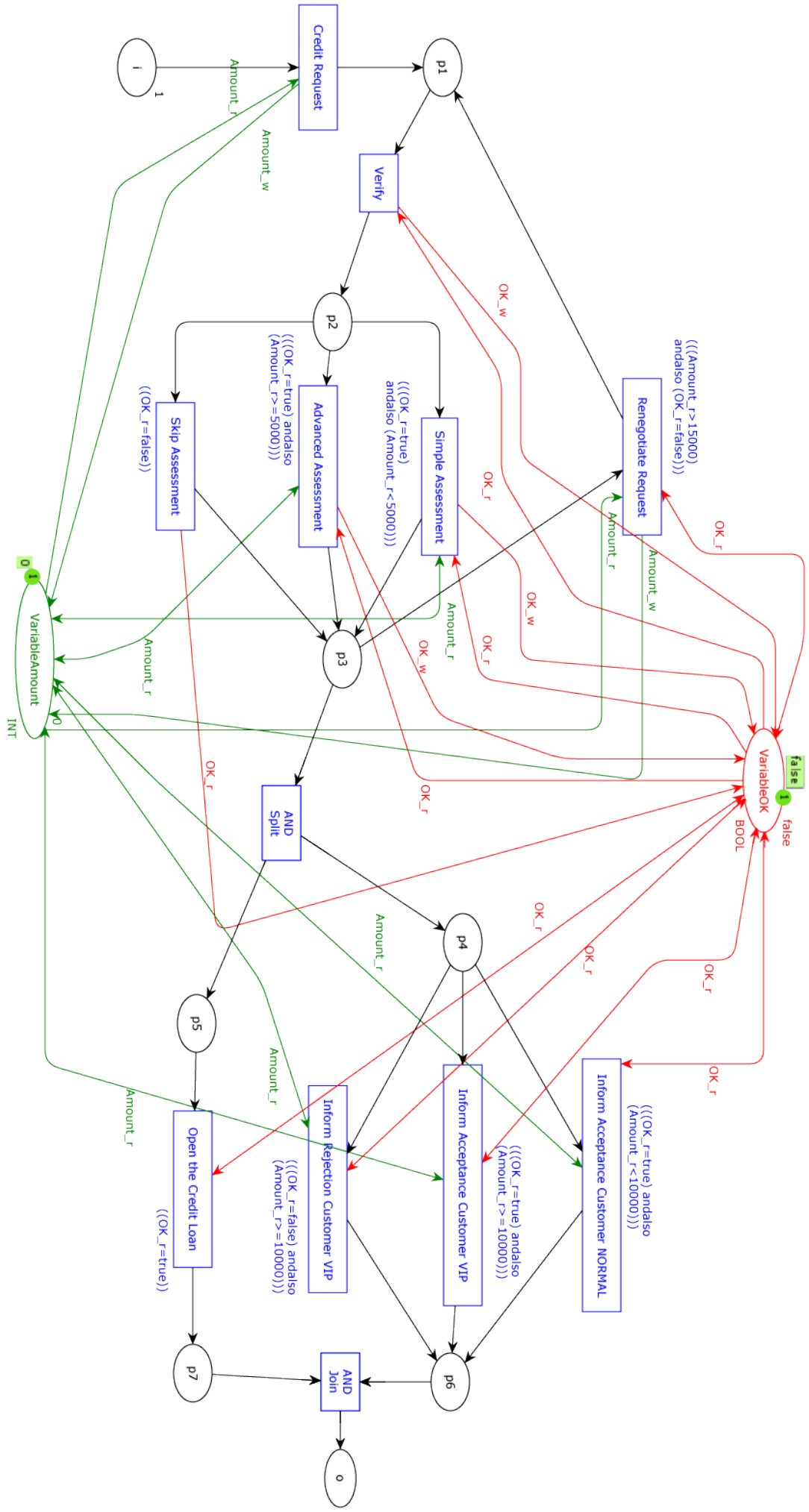
This section illustrates how a DPN can be converted into a CPN . Intuitively, as exemplified in Figure 6, the transitions and places of the DPN become transitions and places of the CPN. Each variable of the DPN becomes one variable place that is associated with the same colorset as the variable type of (place in example in Figure 6 (right). These places always contain exactly one token, holding the current value of the variable. Guards are exactly the same as the guards of the CPN, and if a transition writes a variable , the token in the variable place for is consumed and a new token generated to model that is the value of is updated. For instance, the fact that transition of the DPN Figure 6 (left) writes a new value for variable (denoted ) is modelled in Figure 6 (right) through the two red arcs annotated with and that respectively enters and exits transition : this allows the token holding the value of to change value when returned back to the place. The read operations can be modelled as the blue arcs as in Figure 6 (right), with the same annotation, so that the token from the variable place is consumed and then put back. The initial marking of the DPN becomes part of the initial marking of the CPN: each variable place is initialized with a token that holds the initial value of the variable. In Figure 6 (right), the place contains a token with value , assuming . The following formalizes this intuition.
Places. The places of the CPN consist of all places of the DPN, plus one dedicated extra place , hereafter called variable place, for each DPN variable ;
. A variable place always has one token, and precisely the one holding the current value of variable at each step of the simulation of the CPN.
Transitions. The transitions of the CPN and DPN are the same: .
Arcs. Each arc in is preserved, and for any transition and variable read and/or written in , we add two extra arcs: ,
and the node function is defined as for any .
Color sets. The CPN supports the same variable types as the DPN, and we consider the color sets corresponding to the domains defined at the beginning of Section 3 for integers, reals, booleans and strings, respectively. Variables. For each variable the CPN considers the variables and , i.e.,
, where is the special dummy variable with the only possible value .
Color functions. Recalling the shorthand notation for typed variables in , each place is associated with a color set as follows. If then , otherwise:
Guards. Guards are not changed: for each .
Arc expressions. The expression associated with any arc between a source node
and a target with is as follows. If then , otherwise:
The first case refers to arcs of the CPN that are also present in the original DPN (e.g. in the set of arcs ); the places involved in these arcs contain tokens with no value associated and, which we represent by , and thus the arcs are annotated with the variable. The remaining cases refer to arcs connecting the variable places for each to a transition . If is written by then the incoming arc and the outgoing arc are annotated with and , respectively. This allows the token holding the value of to change value when returned back to .
If instead is not written by then both arcs are annotated with the same inscription , guaranteeing that the value of token does not change.
Initialization. Let be the initial marking of the DPN. Places that are also in the DPN take on the same number of tokens as in the DPN, whereas each variable place is initialized with a token holding the value specified by the initial SV assignment of the DPN. Namely, if , i.e., is a place in the original net, otherwise where .
This translation is correct: a DPN is sound if and only if its translation to CPN is sound, and it also allows one to leverage on standard techniques [21]. Specifically, in this paper we resort on building and analysing the reachability graph of the CPN, on which the conditions as in Definition 6 can be checked as follows: properties P1 and P2 can be assessed by verifying that, for any state of the reachability graph, it is possible to reach a final marking. Property P3 can be checked by assessing whether the reachability graph contains at east one edge for every transition.
Example 4
Figure 7 illustrates how the working example is translated into a CPN. The red the green elements implements the operations of reading and updating (i.e. writing) of the variables and , respectively.
5.2 Taming Infinity via Representatives
However, although the translation is correct, it is easy to see that the reachability graph can have infinitely many distinct states. There source of infiniteness is twofold: on the one hand, the original DPN itself and thus the CPN can have an unbounded number of tokens; on the other hand, the process variables of the original DPN determine color sets in the CPN over possibly infinite domains. While the former can be tackled by standard techniques, the infiniteness of the process data makes them ineffective, and it does not give us any insight on whether soundness can be actually verified and, if so, how.
Definition 8 (Constants of the process)
The set of constants related to a typed variable of a DPN is defined as the set of all the values such that either or appears in any guard of any , with .
Observing that each such set is finite and ordered, for each of these we partition the universe into intervals of values in which can be partitioned wrt , and for each elect a representative, which can be chosen arbitrarily among the values in the interval. To correctly handle the case in which the domain of a variable has no minimal or maximal elements, we define the set as with either or both of these two elements added, when needed. Hence the set of representatives for is computed as: where is a deterministic function returning a representative value in the specified interval, excluding the endpoints.44 4 For dense domains such as real numbers such intervals are always nonempty, whereas for non-dense domains they might be empty. In this case, we consider undefined. For a given value in the original domain , we denote its representative as , namely iff , otherwise implies both and . For , we define .
Let . We define a SV assignment restricted to as a function , with the restriction that for any . Given a SV assignment on the original domain of any variable , we compute its restriction as .
By considering a finite number of representative values, we can verify the soundness of a DPN by checking the soundness of the corresponding CPN if one restricts the values which can be assigned to each to the set . As we are going to show, although this cannot guarantee the reachability graph of the CPN to be finite-state in general, it suitably eliminates the infiniteness originating from the process data. To ensure this, we need to add further constraints to the CPN as follows. For each variable in the DPN, we add an additional place to the set places of the CPN, which is meant to represent the restricted set of possible values of , namely . To this end, is assigned the same colorset as that of the variable place , and it holds one token for each possible representative value in . This is achieved through the initialisation function of , by imposing . Then, for any transition and for each variable , the representative value held by one token in is used to update the value of the token in the variable place .
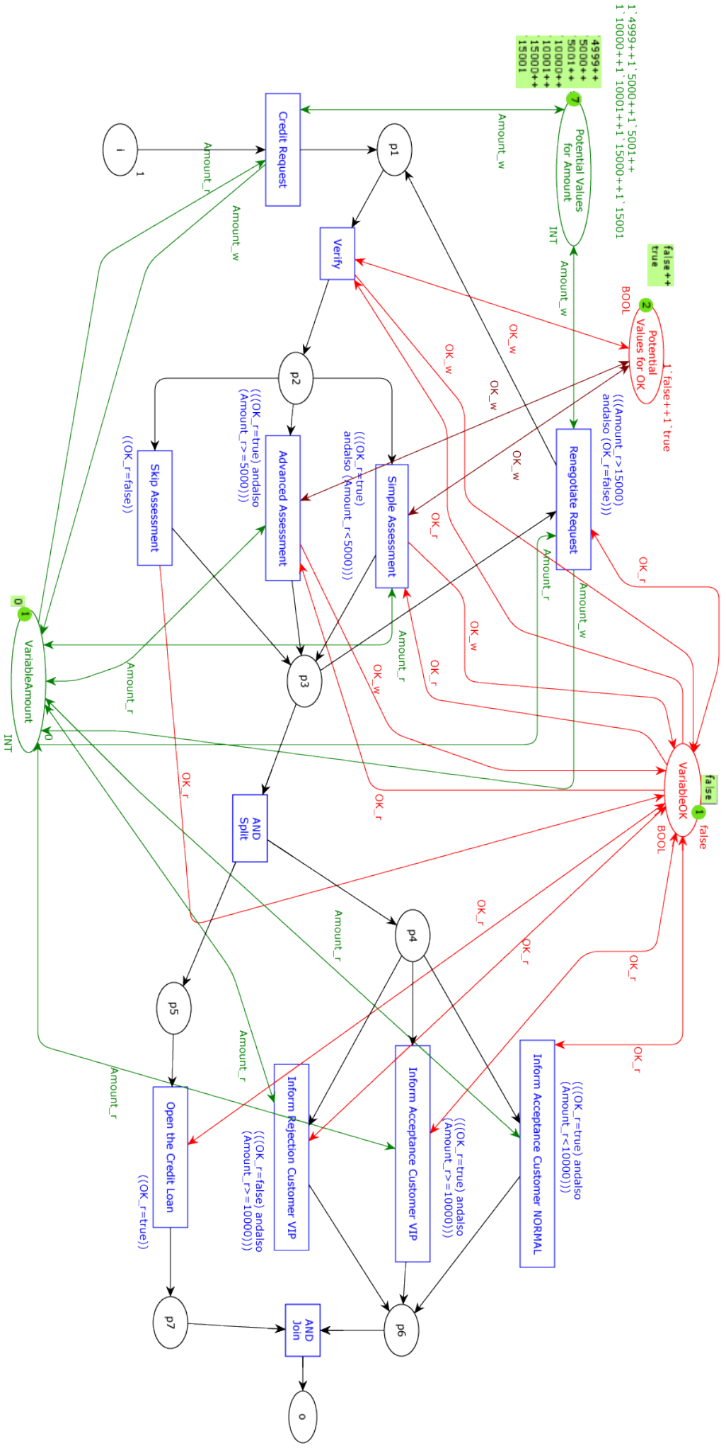
Example 5
Consider, e.g., the transition Credit Request in the model in Figure 7. This transition writes the integer variable . If we inspect all the guards, it is easy to see that the set of constants related to is the set , from which we select the set of representatives by including an arbitrary value for each interval (e.g., in this case, was arbitrarily chosen to represent all the values in the interval ), and a token for each element of is created in . As it can be seen in Figure 8, which depicts the resulting CPN , is called Potential values for Amount and its tokens can be used as possible values for the variable , which the transition Credit Request produces in the variable place , there called VariableAmount.
More formally, we add two arcs to : an arc from to the newly-introduced place and a second arc , and define the expression function so that, for transition and , .
5.3 Correctness of the Translation
We now discuss the correctness of the approach, showing that the CPN defined above preserves the soundness properties of the original DPN. In order to do so, we could show that the CPN built in the previous section (namely obtained by translating the original DPN first into a CPN and thus into ) preserve soundness. This would be hard, as it implies not only comparing a DPN with a CPN that is syntactically very different but also handling infinite domains for case variables. Instead, we first restrict the traces of so as to describe a new DPN through the formal notion of restriction of variable domains introduced before, and only then show that there is indeed a tight relationship between such and the CPN introduced in the last section. This is illustrated in Figure 9.
In the previous section we have shown how any state assignment can be restricted to the state assignment which only selects representatives from for each variable . Intuitively, this allows us to redefine the domain associated to as , and to consider a new DPN that is as the original DPN but in which states are of the form , including the initial state . Similarly, transition firings are as in , with the difference that given a transition firing in , the state assignment for any is if and otherwise.
The following theorem shows that the abstraction step from to depicted in Figure 9 preserves trace-equivalence.
Theorem 5.1
Given a DPN , then is trace-equivalent to .
The intuition behind this result is that for any possible legal process trace of we compare the run of with the run of , with , so that these runs are trace equivalent, where and are the restrictions of and with respect to , for each . Then, we show how for every legal transition firing from the last state of , its restriction is legal from the last state of and that is still trace-equivalent to . The proof proceeds by induction on the length of runs, as the claim trivially holds for runs of length : it is easy to show that if the claim does not hold then either is not legal or it is indeed possible to simply consider the restriction of and thus obtain a run and for which the claim holds. Similarly for the other direction.
Proof
First, observe that the claim holds for runs of length . Then, assume it holds also for runs of length but not for length , and consider and as above. Then it means that for some legal firing from the last state of we cannot find a legal firing from the last state of so that the condition above holds. Or vice-versa. We address these two cases. First, Recall that trace-equivalent runs traverse the same markings, which implies , hence we simply write .
(1): If is legal from but is not legal from , then either cannot be defined as it is not possible to select a representative for for some or the transition firing is not legal from . If is true then but . By definition, this means that and that there are no two consecutive with . This is only possible if the open interval is empty, which contradicts the fact that . If , by definition we have that, considering , either is not satisfied, or it is not true that . If is true then for some either and or is of the form but it is not the case that for . In the former case it follows that also and , while the latter is not possible because if is a constant in then it must be as , whereas if it is a representative value in the interval then there must exist another constant in that is also in , which implies that these are not consecutive constants, unless of course it is also false that . Finally, if () is true then is not legal.
(2:) The proof for the other direction is analogous, proving that for every legal firing from the last state of in there exists a legal firing from the last state of so that is still equivalent to .
We now address the relationship between and the corresponding CPN , built from following the construction illustrated in Section 5.2. As depicted in Figure 9, our goal is to show that the CPN captures all and only the possible runs of , so that we can indeed analyse in ProM, as explained in the next section, to verify properties of the original DPN .
First, with a little abuse of terminology, we extend the notion of trace-equivalence also for comparing DPNs and CPNs.
Definition 9 (Trace-equivalence between DPNs and CPNs)
We say that a DPN run is trace-equivalent to a CPN run iff for each , namely if the runs perform the same transitions ( is the initial marking of the CPN).
Similarly, a DPN and a CPN are trace-equivalent if for every legal run of there exists a trace-equivalent run of and vice-versa.
Theorem 5.2
For any DPN , the corresponding and the CPN defined as in the previous section are trace-equivalent.
It is easy to see that the extra place , included in for any , makes it possible to generate a reachability graph composed of runs that do not distinguish distinct values of variables as long as these are represented by the same representative value in . However, one main difference in addressing the trace-equivalence between a run of a DPN and a run of the corresponding CPN , with respect to the same notion between two DPNs as for the previous theorem, is that their respective markings are structurally different. In markings are of the form whereas for they are computed by a function of the form . We thus need to define a correspondence relation between these two notions of markings, and more precisely between states of a DPN (the same applies to and ) and markings of the corresponding CPN , defined as follows. Given a state of a DPN, for any place we have that and for any we have . Similarly, given a marking of , the corresponding state of the DPN is so that for any place we have and for any we have . With such a notion of correspondence at hand, which we denote by writing , we prove our result.
Proof
(1): We proceed by induction on the length of runs of , with . First, it is easy to see that by construction (see Section 5.1). Then, assume that and that there exists a legal transition firing from such state so that but there is no firing of such that and . Then, either () any possible is not legal from or () it is the case that . The former case is not possible. First, must be enabled in because for every and for any , with arcs between and places and as described in the definition of . Second, we can pick such that for all , which is equivalent to say that for read variables and for written variables . This must be possible or otherwise would not be legal. Third, and for the same reason, if such binding is so that the guard is not satisfied, then the same would hold for (which agrees with for read variables, namely for each ), which would imply that is not legal from . Since it follows that () is also not possible, as and the binding as above is consistent with and : specifically, for places we have , and for places we have , where agrees with the marking , namely selects a value from when , and selects a value from when , with for .
(2): The type of reasoning for the other direction is analogous.
Putting the theorems together, as depicted intuitively in Figure 8, the following theorem holds, as the property of trace-equivalence between runs is clearly transitive.
Theorem 5.3
For any DPN , the corresponding CPN obtained with the construction so far described is trace-equivalent to .
We thus turn to the question of determining whether the property of trace equivalence stated in the previous theorems allow one to transfer interesting properties. However, note that we cannot evaluate the same properties on both and without a translation for CPNs. The translation is intuitive although cumbersome, and it is left to the reader (an example is provided in the next section).
Corollary 1
The soundness properties in Definition 6 hold in iff their translations hold in , hence is sound iff is sound.
The proof is quite intuitive, and relies on observations already used in the proofs above. By the proof of the Theorem 5.1, it follows that the reachability graphs of and have the same branching structure with respect to transitions in : at each step, any task that is enabled in in a given run fragment is also enabled in the corresponding trace-equivalent run in . Similarly, by the proof of Theorem 5.3, trace-equivalent runs of and traverse markings that are in correspondence, as defined earlier. Therefore, at every step, every enabled transition in the must be enabled in the corresponding state of the .
Example 6
Consider again the running example from Example 1 depicted in Figure 1. As already anticipated (see Example 2), the net is unsound as it is possible to reach a deadlock (e.g. having a token in and ). Note that the same happens in its resulting representative CPN which uses representative values, shown in Figure 8. The key point is that, while in the original DPN there exists an infinite number of values (e.g. for the requested credit) for which a deadlock can be reached, all these are correctly represented by a finite number of runs in .
5.4 Relating Data-aware soundness and Decision-aware soundness
The previous result suggests that our technique is in fact not limited to data-aware soundness, but it can be applied to any property that does not rely on specific identity values of case variables (because is insensible to the assignments of variables, as it uses representative values). We consider here the properties in [2] which characterise various notions of decision-aware soundness.
Corollary 2
The truth value of all the properties in [2] is the same in and .
The rest of this section is devoted to support this claim. First, we now look at the decision-aware properties from [2], adapting them to our case, where DMN decisions are represented in a DPN as transitions that are used to model the business rule task that is associated to the decision table (we consider here a unique hit policy for decision tables, see Section 4).
We start by addressing the two fundamental properties of conditional completeness and conditional output coverage. As shown in Section 4.2, a decision fragment is modelled in a DPN as a set of transitions, as exemplified in Figure 4. We denote one such set as , and all these decisions as . This notation allows us to refer to all the transitions that belong to the same decision.
Also, for convenience of notation, given a DPN we consider the set defined as the set for a given DPN , that is, the set of all states reachable through legal runs, which are intrinsically data-aware.
Conditional completeness (P4). As explained in Section 4, decision fragments are captured by transitions with guards encoding the rules of decision tables (see for instance Figure 4). A set of transitions, one for each rule in a table, is therefore said to be conditionally complete iff at least one can legally fire from any reachable state in which it is enabled my the marking. This is captured by the property . . The property simply states that from any reachable state from which transitions corresponding to a decision task are available, then for each decision there exists at least one transition from the same set that is legally executable. It however immediate to see that is implied by , which prescribes that from any reachable state it is always possible to complete the process, irrespective of the SV assignments and thus irrespective of the values of variables that transitions produce along the run.
Conditional output coverage (P5). The property holds for a decision table when all outputs are covered by conditions in the succeeding gateway. In our formalism, this correspond to check that for every possible legal transition firing , from the last state of a legal run fragment, we have that the resulting state is not a dead-end. Hence: . (. . The property is true in iff it is true for all . Again, note that this property is implied by .
State-Based Decision Deadlock Freedom. It requires that every transition , such that is legal from the last state of a legal run fragment, is conditionally complete and all its outputs are conditionally covered. Hence, the property corresponds to checking and .
State-based Dead Branch Absence. It requires that along any branch in each decision fragment there is an output of the decision model such that this branch is selected for execution. As we represent a transitions both the business rule task and the following conditions, this is a relaxation of , limited to those transitions that follow one in .
Decision-Aware Soundness. A DPN is decision-aware sound iff it is classically sound, it is decision deadlock free and state-based dead branch free. Note that, under such conditions, the three properties of classical soundness [3] are guaranteed also with respect to the possible decision-aware paths of the process. In our setting, this corresponds to - together with and . However, recall that implies and , and hence this definition is equivalent to data-aware soundness (Definition 6).
Decision-Aware Relaxed Soundness. It requires relaxed soundness, state-based decision deadlock freedom and state-based dead branch absence. The first specifies that every transition can participate in at least one sound firing sequence, which is captured by and in out setting already implies state-based dead branch absence. The property thus corresponds to , , .
Decision-Aware Weak Soundness. It requires classical weak soundness, which is less strict than decision-aware soundness as it allows dead transitions (although any transition that can fire must always lead to a proper termination) and state-based decision deadlock freedom. As weak soundness is captured by and , the property corresponds to checking , , ( is implied).
Decision-Aware Lazy Soundness. It allows the net to be lazy in the sense that there can be tokens left in the net after a token appeared on the final place (i.e. violating ). When considering our execution semantics, it requires that from every (legally) reachable state the end transition (i.e., leading to the output place of ) can be reached exactly once. We can express this as the conjunction of with a simple relaxation of , namely . .
Decision-Aware Easy Soundness. It requires classical easy soundness and that at least one run (hence trace) to be state-based decision deadlock free and state-based dead branch free. We provide here the most reasonable interpretation of this definition. Since easy soundness simply requires that for at least one token on the initial place a token will eventually appear on the final place, the requirement is captured by checking the existence of at least one run in which a relaxation of holds ( and are guaranteed by the legality of the selected trace). : .
With arguments very similar to those applied for the proof of Theorem 5.3, it can be easily seen that these properties hold in iff they hold in (once rewritten for CPNs), due to trace-equivalence. Indeed, they are all based on legal runs and legally reachable states, which are all accounted for in . We exemplify such reasoning for , as the argument is akin to those for , and .
Proof
(Sketch.) First, we express the corresponding requirement on CPNs for any set of transitions as . Assume that is satisfied in for every set . Then for every run in with for some and we have for some and , which agrees with by construction. Since they are trace-equivalent, this implies that there exists a trace in with for each , which implies that for any place we have and for any we have . Hence it must also be that is enabled in , namely for some and or otherwise the trace-equivalence would be violated. Therefore is satisfied for . A similar argument holds for the other direction.
We conclude by noting that, shown in Figure 10, the same relationships between all the notions presented in [2] are correctly reconstructed, as expected. In particular, as shown in the figure, it turns out that our notion of data-aware soundness for DPNs is equivalent to that of decision-aware soundness for processes associated with DMN decision models. That is, if we either (a) check decision-aware soundness on processes with DMN decisions or (b) translate them into a DPNs and then check data-aware soundness, then we get the same result. This supports the claim that data-aware soundness in indeed suitable for capturing the soundness of Petri net-based process models enriched with case data and decisions. It requires the existence of at least one way of completing a process through the execution of a legal sequence of transition firings, in any possible case that is allowed by both the control-flow and the data-flow of the process. This is a very strong property: it is guaranteed irrespective of the values that may be written along the execution.
At the same time, note that data-aware soundness does not rely on the specific structure of the process: while decision-aware soundness, as studied in [2], assumes that decisions are represented as decision fragments, thus fixing a specific shape of the process, data-aware soundness is evaluated on generic DPNs. This allows one to consider processes with arbitrary conditions on the data they manipulate, which makes our approach more general. Moreover, the execution semantics defined here is itself data-aware, as opposed to imposing additional requirements on the decision tables, in addition to checking classical soundness.
6 Implementation And Experiments


Our soundness-checking technique has been implemented as a Java plug-ins for ProM, an established open-source framework for implementing process mining algorithms and tools (see http://www.promtools.org/), which supports both the PNML and the BPMN file formats to load process models in those two formats. ProM also implements numerous algorithms for discovering process models that integrate the decision perspective (e.g. [8]). Thanks to this, we can employ our technique to validate the soundness of models where the decision perspective is mined from event data and models can be expressed in the two mentioned notations. In particular, the soundness-checking technique is available in the ProM nightly build after ensuring that the ProM package DataPetriNets is installed. The plug-in is named Compute Soundness of a Data Petri Net and takes a DPN as input. Figure 11 refers to the output for the working example in Figure 1. The output illustrates the list of dead transitions as well as the undesired deadlocks, namely the list of markings in which no transitions are enabled although they are not final. For the working example the only undesired deadlock is the marking with one token in and . Clicking on the deadlock, at the bottom the plug-in shows an example of execution that leads to that marking, namely when is 5000 and is false.
We performed a number of experiments with data-aware models of real-life processes that were used in previous publications and theses:
- 1.
We used the model of the real-life process for the management of road-traffic fines, which is illustrated in Figures 7 and 8 of [14]. Space limitation prevents us from showing the models here. Figure 12 shows the feedback screen the ProM plug-in for soundness checking: no transition is dead and two deadlock markings can be identified. By clicking on any of the deadlock, an example of execution that leads to that deadlock is shown at the bottom. By inspecting the model, one can easily observe that the deadlock at the top (i.e. with a token in place ) is caused by the fact that transition Appeal to Judge can assign any value to variable dismissal. This transition is followed by a XOR split where two alternative transitions are possible, depending on the value of variable dismissal: NIL or #. However, the model does not impede Appeal to Judge to assign other values, e.g. G, thereby causing a deadlock.
- 2.
We checked the soundness of the data-aware models reported in Figures 13.6 and 15.6 of the Ph.D. thesis by Mannhardt [13]. Both models refer to processes that are executed within hospitals: the former is about curing patients with sepsis and the latter manages the hospital billing to patients. These models were partly hand designed and partly mined through process-discovery techniques.
Figure 13: A data-aware Petri Net that models a road-traffic fine management process. The structure of the transitions and places of the net is manually designed and the guards are discovered through decision-mining techniques. The read and write operations are not shown and long guards are partly cut in order to maintain some readability. - 3.
We use the same model as at point 1 but, instead of keeping in the pre-existing guards, we employed the guard discovery technique discussed in [15], which does not formally guarantee that the discovered models comply the properties of Definition 6. The resulting model is in Figure 13, which is data-aware sound. The analysis has not indeed reported dead transitions or deadlocks.
The models at points 1 and 2 were analysed for deadlocks and dead transitions in a matter of seconds. The model at point 3 required 1.9 hours to return the analysis results. This difference is due to the fact that the model at point 3 is likely over-precise for what concerns the decisions. Therefore, the decisions are modelled through complex guards with several atoms; as a consequence, the search space to visit grows significantly.
7 Conclusions
In this paper we have introduced a holistic, formal and operational approach to verify the end-to-end soundness of Data Petri nets, which we called data-aware soundness. Thanks to the solid formal foundation of DPNs, we defined a notion of soundness for these nets to incorporate the decision perspective, and developed a technique for assessing such property that can be directly implemented on existing tools. We also characterised how our definition of data-aware soundness is related to known notions of decision-aware soundness in the literature. In future work, we plan to address more sophisticated guard languages than the one considered in this paper, for instance by allowing to compare variables through guards such as . Note however that this goes beyond DMN S-FEEL and thus requires more sophisticated encoding techniques, although we believe this to be a decidable setting. Further, we aim at extending our results to other data domains. This is a quite delicate task, since even minimal extensions may lead to undecidability. For instance, by enriching integer domains by a successor predicate, we immediately get an undecidability result for soundness, even in the simple case of DPNs with two case variables. Finally, we also have some intriguing ideas on how to optimize the technique presented in this paper. In its current form, nondeterminism is managed eagerly, that is, by generated branches for possible values as soon as a variable is written. It appears instead promising to manage nondeterminism lazily, i.e., by postponing such choice to the moment where the variable actually appears in a guard, hence considering sets of possible representatives at the same time. This would not preserve trace-equivalence, but could still preserve soundness.
References
- [1] Decision model and notation (DMN) v1.1, 2016.
- [2] K. Batoulis, S. Haarmann, and M. Weske. Various notions of soundness for decision-aware business processes. In Proc. of ER 2017, volume 10650 of LNCS, pages 403–418. Springer, 2017.
- [3] K. Batoulis and M. Weske. Soundness of decision-aware business processes. In Proc. of BPM Forum 2017, pages 106–124. Springer, 2017.
- [4] D. Calvanese, G. De Giacomo, and M. Montali. Foundations of data aware process analysis: A database theory perspective. In Proc. of PODS 2013. ACM, 2013.
- [5] D. Calvanese, M. Dumas, Ü. Laurson, F. M. Maggi, M. Montali, and I. Teinemaa. Semantics and analysis of DMN decision tables. volume 9850 of LNCS, pages 217–233. Springer, 2016.
- [6] E. M. Clarke, O. Grumberg, and D. E. Long. Model checking and abstraction. ACM Trans. Program. Lang. Syst., 16(5):1512–1542, 1994.
- [7] M. de Leoni, J. Munoz-Gama, J. Carmona, and W. M. P. van der Aalst. Decomposing Alignment-Based Conformance Checking of Data-Aware Process Models, pages 3–20. Springer, 2014.
- [8] M. de Leoni and W. M. P. van der Aalst. Data-aware process mining: Discovering decisions in processes using alignments. In SAC 2013, pages 1454–1461. ACM, 2013.
- [9] R. M. Dijkman, M. Dumas, and C. Ouyang. Semantics and analysis of business process models in BPMN. Information & Software Technology, 50(12):1281–1294, 2008.
- [10] K. Jensen and L. M. Kristensen. Coloured Petri Nets: Modelling and Validation of Concurrent Systems. Springer Publishing Company, Incorporated, 1st edition, 2009.
- [11] A. A. Kalenkova, W. M. P. van der Aalst, I. A. Lomazova, and V. A. Rubin. Process mining using bpmn: Relating event logs and process models. In Proc. of MODELS 2016, pages 123–123. ACM, 2016.
- [12] D. Knuplesch, L. T. Ly, S. Rinderle-Ma, H. Pfeifer, and P. Dadam. On enabling data-aware compliance checking of business process models. volume 6412 of LNCS, pages 332–346. Springer, 2010.
- [13] F. Mannhardt. Multi-perspective process mining. Ph.d. thesis, Eindhoven University of Technology, 2018. http://repository.tue.nl/b40869c0-2d11-4016-a92f-8e4ee9cd9d66.
- [14] F. Mannhardt, M. de Leoni, H. A. Reijers, and W. M. P. van der Aalst. Balanced multi-perspective checking of process conformance. Computing, 98(4):407–437, Apr 2016.
- [15] F. Mannhardt, M. de Leoni, H. A. Reijers, and W. M. P. van der Aalst. Decision mining revisited - discovering overlapping rules. In CAiSE 2016, volume 9694 of LNCS, pages 377–392. Springer, 2016.
- [16] M. Montali and D. Calvanese. Soundness of data-aware, case-centric processes. Int. Journal on Software Tools for Technology Transfer, 2016.
- [17] A. V. Ratzer, L. Wells, H. M. Lassen, M. Laursen, J. F. Qvortrup, M. S. Stissing, M. Westergaard, S. Christensen, and K. Jensen. Cpn tools for editing, simulating, and analysing coloured petri nets. In Proceedings of the 24th International Conference on Applications and Theory of Petri Nets, ICATPN’03, pages 450–462. Springer, 2003.
- [18] S. Sadiq, M. Orlowska, W. Sadiq, and C. Foulger. Data flow and validation in workflow modelling. In Proceedings of the 15th Australasian Database Conference - Volume 27, Proc. of ADC ’04, pages 207–214, Darlinghurst, Australia, Australia, 2004. Australian Computer Society, Inc.
- [19] N. Sidorova, C. Stahl, and N. Trčka. Workflow soundness revisited: Checking correctness in the presence of data while staying conceptual. In Proceedings of the 22Nd International Conference on Advanced Information Systems Engineering, Proc. of CAiSE 2010, pages 530–544. Springer, 2010.
- [20] N. Sidorova, C. Stahl, and N. Trčka. Soundness verification for conceptual workflow nets with data: Early detection of errors with the most precision possible. Information Systems, 36(7):1026–1043, 2011.
- [21] W. M. P. van der Aalst. The application of petri nets to workflow management. Journal of Circuits, Systems, and Computers, 8(1):21–66, 1998.