Quantum Dynamics with the Parallel Transport Gauge

Dong An ^†^†thanks: Department of Mathematics, University of California, Berkeley, Berkeley, CA 94720. Email: dong_an@berkeley.edu Lin Lin ^†^†thanks: Department of Mathematics, University of California, Berkeley, Berkeley, CA 94720 and Computational Research Division, Lawrence Berkeley National Laboratory, Berkeley, CA 94720. Email: linlin@math.berkeley.edu

Abstract

The dynamics of a closed quantum system is often studied with the direct evolution of the Schrödinger equation. In this paper, we propose that the gauge choice (i.e. degrees of freedom irrelevant to physical observables) of the Schrödinger equation can be generally non-optimal for numerical simulation. This can limit, and in some cases severely limit the time step size. We find that the optimal gauge choice is given by a parallel transport formulation. This parallel transport dynamics can be simply interpreted as the dynamics driven by the residual vectors, analogous to those defined in eigenvalue problems in the time-independent setup. The parallel transport dynamics can be derived from a Hamiltonian structure, thus suitable to be solved using a symplectic and implicit time discretization scheme, such as the implicit midpoint rule, which allows the usage of a large time step and ensures the long time numerical stability. We analyze the parallel transport dynamics in the context of the singularly perturbed linear Schrödinger equation, and demonstrate its superior performance in the near adiabatic regime. We demonstrate the effectiveness of our method using numerical results for linear and nonlinear Schrödinger equations, as well as the time-dependent density functional theory (TDDFT) calculations for electrons in a benzene molecule driven by an ultrashort laser pulse.

keywords

Schrödinger equation; Quantum dynamics; Gauge; Parallel transport; Density matrix; von Neumann equation; Symplectic method; Singularly perturbed system; Time-dependent density functional theory; Adiabatic theorem

1 Introduction

Consider the following set of coupled nonlinear Schrödinger equations

\mathrm{i}\epsilon\partial_{t}\Psi(t)=H(t,P)\Psi(t).\\

(1.1)

Here we assume $0<\epsilon\ll 1$ . $\Psi(t)=[\psi_{1}(t),\ldots,\psi_{N}(t)]$ are $N$ time-dependent wave functions subject to suitable initial and boundary conditions. $H(t,P)$ is a self-adjoint time-dependent Hamiltonian. $P(t)$ is called the density matrix and defined as

P(t)=\Psi(t)\Psi^{*}(t)=\sum_{j=1}^{N}\psi_{j}(t)\psi_{j}^{*}(t).

(1.2)

Note that when the initial state $\Psi(0)$ consists of $N$ orthonormal functions, the functions in $\Psi(t)$ will remain orthonormal for all $t$ , i.e. $(\psi_{i}(t),\psi_{j}(t))=\delta_{ij}$ , where $(\cdot,\cdot)$ denotes a suitable inner product. Then

P^{2}(t)=\sum_{j,k=1}^{N}\psi_{j}(t)(\psi_{j}(t),\psi_{k}(t))\psi_{k}^{*}(t)=\sum_{j=1}^{N}\psi_{j}(t)\psi_{j}^{*}(t)=P(t),

i.e. $P(t)$ is a projector. The explicit dependence of the Hamiltonian on $t$ is often due to the existence of an external field, and we assume the partial derivatives $\frac{\partial^{m}H}{\partial t^{m}}$ are of $\mathcal{O}(1)$ in some suitable norms for all $m\geq 1$ . Hence when $0<\epsilon\ll 1$ , the wave functions can oscillate on a much smaller time scale than that of the external fields, and this is called the singularly perturbed regime [13].

The equations (1.1) are rather general and appear in several fields of scientific computation. In the simplest setup when $N=1$ and $H(t,P)\equiv H(t)$ , this is the linear Schrödinger equation. Another example is the nonlinear Schrödinger equation (NLSE) used for modeling nonlinear photonics and Bose-Einstein condensation process [10],

\mathrm{i}\epsilon\partial_{t}\psi(t)=H_{0}(t)\psi(t)+g|\psi(t)|^{2}\psi(t){,}

(1.3)

where $H_{0}(t)$ is a Hermitian matrix obtained by discretizing the linear operator $-\frac{1}{2}\Delta+V(x,t)$ . Since $N=1$ , $P(t)=\psi(t)\psi^{*}(t)$ , and $|\psi(t)|^{2}=\mathrm{diag}[P(t)]$ is a nonlinear local potential. When $N>1$ , the coupled set of Schrödinger equations must be solved simultaneously. This is the case in the time-dependent density functional theory (TDDFT) [34, 32].

The simulation of Eq. (1.1) and in particular (1.3) has been studied via a wide range of numerical discretization methods, such as explicit Runge-Kutta methods [36], implicit Runge-Kutta methods [6], operator splitting methods [3, 27], Magnus expansion methods [6, 7], exponential time differencing methods [21], spectral deferred correction methods [19], dynamical low rank approximation [24], adiabatic state expansion [18, 39], to name a few. What this paper focuses on is not to develop another numerical scheme to directly discretize (1.1), but to propose an alternative formulation that is equivalent to (1.1), and can be solved with improved numerical efficiency using existing discretization schemes.

More specifically, note that if we multiply $\Psi(t)$ by a time-dependent unitary matrix $U(t)\in\mathbb{C}^{N\times N}$ , the resulting set of rotated wave functions, denoted by $\Phi(t)=\Psi(t)U(t)$ , yields the same density matrix as

P(t)=\Phi(t)\Phi^{*}(t)=\Psi(t)\left[U(t)U^{*}(t)\right]\Psi^{*}(t)=\Psi(t)\Psi^{*}(t).

(1.4)

Since the unitary rotation matrix $U(t)$ is irrelevant to the density matrix which is used to represent many physical observables, $U(t)$ is called the gauge, and Eq. (1.4) indicates the density matrix is gauge-invariant. Furthermore, Eq. (1.1) can be directly written in terms of the density matrix as

\mathrm{i}\epsilon\partial_{t}P(t)=[H(t,P),P(t)],

(1.5)

where $[H,P]:=HP-PH$ is the commutator between $H$ and $P$ . Eq. (1.5) is called the von Neumann equation (or quantum Liouville equation), which can be viewed as a more intrinsic representation of quantum dynamics since the gauge degrees of freedom are eliminated completely.

The simulation of the von Neumann equation can also be advantageous from the perspective of time discretization. Consider the simplified scenario that $H(t,P)\equiv H(P)$ does not explicitly depend on $t$ , and the initial state $\Psi(0)$ consists of a set of eigenfunctions of $H$ , i.e.

H[P]\psi_{j}(0)=\psi_{j}(0)\lambda_{j}(0),\quad j=1,\ldots,N,\quad P=\sum_{j=1}^{N}\psi_{j}(0)\psi_{j}^{*}(0).

(1.6)

Eq. (1.6) is a set of nonlinear eigenvalue equations. When solved self-consistently, the solution to the Schrödinger equation (1.1) has an analytic form

\psi_{j}(t)=\exp\left(-\frac{\mathrm{i}}{\epsilon}\lambda_{j}(0)t\right)\psi_{j}(0),\quad j=1,\ldots,N,

(1.7)

which oscillates on the $\mathcal{O}(\epsilon)$ time scale. Hence many numerical schemes still need to resolve the dynamics with a time step of $\mathcal{O}(\epsilon)$ . On the other hand, the right hand side of the von Neumann equation vanishes for all $t$ , and hence nominally can be discretized with an arbitrarily large time step! Of course one can use techniques such as integration factors [8] to make this simulation using the Schrödinger equation as efficient. However this example illustrates that the gap in terms of the size of the time step generally exists between the Schrödinger representation and the von Neumann representation.

In this paper, we identify that such gap is solely due to the gauge degrees of freedom in the Schrödinger representation. By optimizing the gauge choice, one can propagate the wave functions using a time step comparable to that of the von Neumann equation. We demonstrate that the optimized gauge is given by a parallel transport (PT) formulation. We refer to this gauge as the parallel transport gauge, and the resulting dynamics as the parallel transport dynamics. Correspondingly the trivial gauge $U(t)\equiv I_{N}$ in Eq. (1.1) is referred to as the Schrödinger gauge, and the resulting dynamics as the Schrödinger dynamics. We remark that the PT dynamics can also be interpreted as an analytic and optimal way of performing the dynamical low rank approximation [24] for Eq. (1.1). Note that the simulation of the von Neumann equation requires the explicit operation on the density matrix $P(t)$ . When a large basis set such as finite elements or planewaves is used to discretize the partial differential equation, the storage cost of $P(t)$ can be often prohibitively expensive compared to that of the wave functions $\Psi(t)$ . Hence the PT dynamics combines the advantages of both approaches, namely to perform simulation using the time step size of the von Neumann equation, but with cost comparable to that of the Schrödinger equation.

We analyze the effectiveness of the PT dynamics for the linear time-dependent Schrödinger equation in the near adiabatic regime. We remark that efficient numerical methods have been recently developed in this regime based on the construction of a set of instantaneous adiabatic states [18, 39]. The assumption is that the wave functions can be approximated by the subspace spanned by low energy eigenstates of the Hamiltonian at each $t$ . The dimension of the subspace is often chosen to be $cN$ , where $c$ is a relatively small constant. Compared to these methods, the PT dynamics always operates only on $N$ wave functions, and therefore has reduced computational and the storage cost. The PT dynamics is also applicable beyond the near adiabatic regime.

By extending the quantum adiabatic theorem [29, 2] to the PT dynamics, we prove that the local truncation error of the PT dynamics gains an extra order of accuracy in terms of $\epsilon$ , when the time step is $\mathcal{O}(\epsilon)$ or smaller. The PT dynamics, after a slight modification, can be derived from a Hamiltonian system similar to that in the Schrödinger dynamics. Hence the gain of accuracy for the local truncation error can be directly translated to the global error as well for long time simulation.

We demonstrate the effectiveness of the PT dynamics using numerical results of the model linear and nonlinear Schrödinger equations. We also perform time-dependent density functional theory (TDDFT) calculations for the electrons in a benzene molecule driven by an ultrashort laser pulse, near and beyond the adiabatic regime. When the spectral radius of the Hamiltonian is large, it is suitable to discretize the PT dynamics using a symplectic and implicit time discretization scheme, such as the implicit midpoint rule, and the resulting scheme can significantly outperform the same scheme for the Schrödinger dynamics. We also find that other time-reversible and implicit time discretization schemes, such as the Crank-Nicolson scheme, can yield similar performance as well. Numerical results confirm our analysis in the near adiabatic regime, and indicate that the convergence of the PT dynamics can start when the time step size is much larger than $\mathcal{O}(\epsilon)$ . This is in contrast to the Schrödinger dynamics where the error stays flat until the time step reaches below $\mathcal{O}(\epsilon)$ . For TDDFT calculations, we find that our discretized PT dynamics can achieve $31.7$ times speedup in the near adiabatic regime, and $5.3$ times speedup beyond the adiabatic regime.

This paper is organized as follows. We derive the parallel transport gauge in Section 2, and discuss the numerical discretization of the parallel transport dynamics in Section 3. We analyze the parallel transport dynamics in the singularly perturbed regime in Section 4. We then present the numerical results in Section 5, followed by the conclusion in Section 6.

2 Parallel Transport Gauge

Since the concept of the parallel transport gauge is associated with the time propagation instead of spatial discretization, for simplicity of the presentation, unless otherwise specified, we assume that Eq. (1.1) represents a discrete, finite dimensional quantum system, i.e. for a given time $t$ , $\psi_{j}(t)$ is a finite dimensional vector, and $H(t,P)$ is a finite dimensional matrix. If the quantum system is spatially continuous, we may first find a set of orthonormal bases functions $\{e_{j}(\mathbf{r})\}_{j=1}^{d}$ satisfying $\int e_{j}^{*}(\mathbf{r})e_{j^{\prime}}(\mathbf{r})\,\mathrm{d}\mathbf{r}=\delta_{jj^{\prime}}$ , and expand the continuous wavefunction as $\widetilde{\psi}_{j}(\mathbf{r},t)\approx\sum_{j=1}^{d}\psi_{j}(t)e_{j}(\mathbf{r})$ . Then after a Galerkin projection, Eq. (1.1) becomes a $d$ -dimensional quantum system, and the inner product for the coefficients $\psi_{j}(t)$ becomes the standard $\ell^{2}$ -inner product as $(\psi_{j}(t),\psi_{k}(t)):=\psi_{j}^{*}(t)\psi_{k}(t)=\delta_{jk}$ . Hence we can use the linear algebra notation. The star notation is interpreted as the complex conjugation when applied to a scalar, and Hermitian conjugation when applied to a vector or a matrix.

2.1 Derivation

For simplicity let us consider the case $N=1$ first, where the gauge matrix $U(t)$ simply becomes a phase factor $c(t)\in\mathbb{C}$ , $|c(t)|=1$ . Note that the gauge choice cannot affect physical observables such as the density matrix. Hence conceptually we may think that the time-dependent density matrix $P(t)$ has already been obtained as the solution of the von Neumann equation (1.5) on some time interval $[0,T]$ . Similarly the wave function $\psi(t)$ satisfying the Schrödinger dynamics is also known. Then the relation

P(t)\varphi(t)=\varphi(t),\quad\varphi(t)=\psi(t)c(t)

(2.1)

is satisfied for any gauge choice. For simplicity we use the notation $\dot{\varphi}(t)=\partial_{t}\varphi(t)$ , and drop the explicit $t$ -dependence in all quantities, as well as the $P$ -dependence in the Hamiltonian unless otherwise noted. Our goal is to find the time-dependent gauge factor $c(t)$ so that the rotated wave function $\varphi(t)$ varies as slowly as possible. This gives rise to the following minimization problem,

\begin{split}\min_{c(t)}\quad&\lVert\dot{\varphi}(t)\rVert^{2}_{2}\\ \text{s.t.}\quad&\varphi(t)=\psi(t)c(t),\quad\lvert c(t)\rvert=1.\end{split}

(2.2)

In order to solve (2.2), note that $P(t)$ is a projector, we split $\dot{\varphi}$ into two orthogonal components,

\dot{\varphi}=P\dot{\varphi}+(I-P)\dot{\varphi}.

(2.3)

By taking the time derivative with respect to both sides of the first equation in Eq. (2.1), we have

(I-P)\dot{\varphi}=\dot{P}\varphi.

(2.4)

Then

\begin{split}\|\dot{\varphi}\|_{2}^{2}&=\|P\dot{\varphi}\|_{2}^{2}+\|(I-P)\dot{\varphi}\|_{2}^{2}\\ &=\|P\dot{\varphi}\|_{2}^{2}+\|\dot{P}\varphi\|_{2}^{2}\\ &=\|P\dot{\varphi}\|_{2}^{2}+\|\dot{P}\psi\|_{2}^{2}.\end{split}

(2.5)

In the last equality, we have used that $\lvert c(t)\rvert=1$ . Note that the term $\|\dot{P}\psi\|_{2}^{2}$ is independent of the gauge choice, so $\|\dot{\varphi}\|_{2}^{2}$ is minimized when

P\dot{\varphi}=0.

(2.6)

Therefore instead of writing down the minimizer of Eq. (2.2) directly, we define the gauge implicitly through Eq. (2.6).

Let us write down an equation for $\varphi(t)$ directly. Combining equations (2.4), (2.6), (1.5) and (2.1), we have

\dot{\varphi}=\dot{P}\varphi=\frac{1}{\mathrm{i}\epsilon}[H,P]\varphi=\frac{1}{\mathrm{i}\epsilon}(H\varphi-\varphi(\varphi^{*}H\varphi)),

(2.7)

or equivalently

\mathrm{i}\epsilon\partial_{t}\varphi=H\varphi-\varphi(\varphi^{*}H\varphi).

(2.8)

For reasons that will become clear shortly, we refer to this gauge choice as the parallel transport gauge, and Eq. (2.8) as the parallel transport (PT) dynamics. Comparing with the Schrödinger dynamics, we find that the PT dynamics only introduces one extra term $\varphi(\varphi^{*}H\varphi)$ . The right hand side of Eq. (2.8) takes the form of the residual vector in the solution of eigenvalue problem of the form (1.6). Hence the PT dynamics can be simply interpreted as the dynamics driven by the residuals. Therefore we expect that the PT dynamics can be particularly advantageous in the near adiabatic regime [18, 39], i.e. when $\varphi$ is close to be the eigenstate of $H$ , and all the residual vectors are therefore small.

Now we provide an alternative interpretation of the gauge choice using the parallel transport formulation associated with a family of projectors. For simplicity let us assume $H(t)$ is already discretized into a finite dimensional Hermitian matrix for each $t$ and so is $P(t)$ . Given the single parameter family of projectors $\{P(t)\}$ defined on some interval $[0,T]$ , we define

\mathcal{A}(t)=\mathrm{i}\epsilon[\partial_{t}P(t),P(t)].

(2.9)

It can be directly verified that $\mathcal{A}(t)$ is a Hermitian matrix for each $t$ , and induces a dynamics

\mathrm{i}\epsilon\partial_{t}\mathcal{T}(t)=\mathcal{A}(t)\mathcal{T}(t),\quad\mathcal{T}(0)=I.

(2.10)

$\mathcal{T}(t)$ is a unitary matrix for each $t$ . $\mathcal{T}(t)$ is called the parallel transport evolution operator (see e.g. [28, 9]). The connection between the parallel transport dynamics and the parallel transport evolution operator is given in Proposition 1.

Proposition 1.

Define $\varphi(t)=\mathcal{T}(t)\psi(0)$ where $\mathcal{T}(t)$ is the evolution operator satisfying (2.10), and $P(t)$ satisfies the von Neumann equation (1.5). Then $P(t)=\varphi(t)\varphi^{*}(t)$ , and $\varphi(t)$ satisfies the parallel transport dynamics (2.8).

Proof.

First we prove the following relation

P(t)\mathcal{T}(t)=\mathcal{T}(t)P(0)

(2.11)

by showing that both sides solve the same initial value problem. Note that $\mathcal{T}(t)P(0)$ satisfies a differential equation of the form (2.10) with the initial value $\mathcal{T}(0)P(0)$ . We would like to derive the differential equation $P(t)\mathcal{T}(t)$ satisfies. Taking the time derivative on both sides of the identity $P(t)=P^{2}(t)$ , we yield two useful relations

\dot{P}=\dot{P}P+P\dot{P},\quad P\dot{P}P=0.

(2.12)

Then using Eq. (2.10),

\mathrm{i}\epsilon\partial_{t}(P\mathcal{T})=\mathrm{i}\epsilon\dot{P}\mathcal{T}+\mathrm{i}\epsilon P[\dot{P},P]\mathcal{T}=\mathrm{i}\epsilon\dot{P}P\mathcal{T}.

On the other hand,

\mathcal{A}(P\mathcal{T})=\mathrm{i}\epsilon(\dot{P}PP\mathcal{T}-P\dot{P}P\mathcal{T})=\mathrm{i}\epsilon\dot{P}P\mathcal{T}.

Therefore

\mathrm{i}\epsilon\partial_{t}(P\mathcal{T})=\mathcal{A}(P\mathcal{T}).

(2.13)

Hence $P\mathcal{T}$ also satisfies an equation of the form (2.10). This proves Eq. (2.11) by noticing further the shared initial condition $P(0)\mathcal{T}(0)=\mathcal{T}(0)P(0)$ .

Using Eq. (2.11), we have

P(t)\varphi(t)=P(t)\mathcal{T}(t)\psi(0)=\mathcal{T}(t)P(0)\psi(0)=\mathcal{T}(t)\psi(0)=\varphi(t).

(2.14)

Since $\mathcal{T}(t)$ is unitary, we have $\lVert\varphi(t)\rVert_{2}=1$ for all $t$ . Hence

P(t)=\varphi(t)\varphi^{*}(t).

(2.15)

The only thing left is to show that the gauge choice in $\varphi(t)$ is indeed the parallel transport gauge. Using Eq. (2.11) and (2.13), we have

\mathrm{i}\epsilon\partial_{t}\varphi=\mathrm{i}\epsilon\partial_{t}(\mathcal{T}\psi(0))=\mathrm{i}\epsilon\partial_{t}(P\mathcal{T})\psi(0)=\mathrm{i}\epsilon\dot{P}P\mathcal{T}\psi(0)=HP\varphi-PHP\varphi.

(2.16)

Here we have used the von Neumann equation

\mathrm{i}\epsilon\dot{P}=HP-PH.

Finally using Eq. (2.14) and (2.15), we have

\mathrm{i}\epsilon\partial_{t}\varphi=H\varphi-\varphi(\varphi^{*}H\varphi),

which is precisely the parallel transport dynamics. ∎

In order to see why the parallel transport gauge can be more advantageous, consider again the time-independent example (1.6) in the introduction for the case $N=1$ . We find that the right hand side of Eq. (2.8) vanishes, and the solution is simply

\varphi(t)=\varphi(0)=\psi(0)

for all $t$ . This implies that the parallel transport gauge is $c(t)=\exp\left(+\frac{\mathrm{i}}{\epsilon}\lambda(0)t\right)$ that perfectly cancels with the rotating factor in (1.7). Hence the PT dynamics yields the slowest possible dynamics by completely eliminating the time-dependent phase factor, and the time step for propagating the PT dynamics can be chosen to be arbitrarily large as in the case of the von Neumann equation.

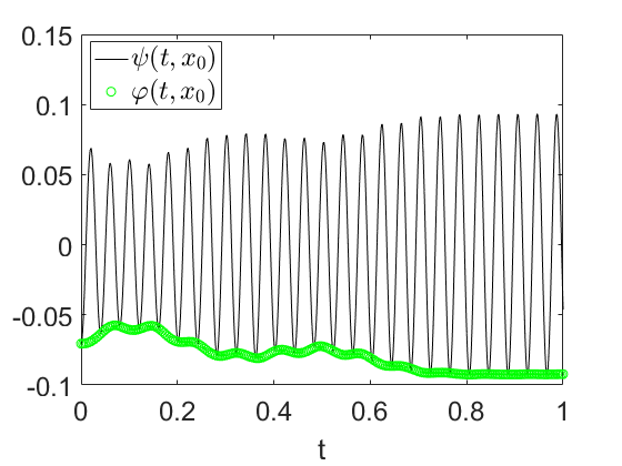
For a more complex example, consider a time-dependent nonlinear Schrödinger equation in one dimension to be further illustrated in Section 5. Fig. 2.1 (a) shows the evolution of the real part of the solution $\psi(t)$ from the Schrödinger dynamics, and that of $\varphi(t)$ from the PT dynamics, respectively. We find that the trajectory of $\varphi(t)$ varies considerably slower than that of $\psi(t)$ , which allows us to use a much larger time step for the simulation. Fig. 2.1 (b) measures the accuracy of the average of the orbital center $\left\langle x\right\rangle(t)$ , using simulation with the implicit midpoint rule, also known as the Gauss-Legendre method of order 2 (GL2) scheme. We compare the performance of the GL2 scheme with the Schrödinger gauge (S-GL2) and that with the PT gauge (PT-GL2) with the same step size $h=0.004$ , and the reference solution is obtained using a very small step size $h=10^{-5}$ . We observe that the solution from PT-GL2 agrees very well with the reference solution, while the phase error of the solution from S-GL2 becomes noticeable already after $t=0.2$ .

2.2 Hamiltonian structure

For simplicity let us consider the linear Schrödinger equation, i.e. $H(t,P)\equiv H(t)$ , and assume $H(t)$ is a real symmetric matrix for all $t$ . It is well known that the Schrödinger dynamics is a Hamiltonian system [30, 31, 11]. More specifically, we separate the solution $\psi$ into its real and imaginary parts as

\psi=q+\mathrm{i}p.

(2.17)

The $\ell^{2}$ -inner product associated with real quantities such as $p,q$ are denoted by $(p,q):=p^{T}q$ . We also introduce the canonically conjugate pair of variables $(\tau,E)$ to eliminate the explicit dependence of $H(t)$ on time [5, 11]. This gives the following energy functional

\mathcal{E}(\tau,q,E,p)=\frac{1}{2\epsilon}\left[q^{T}H(\tau)q+p^{T}H(\tau)p\right]+E.

(2.18)

The Hamiltonian system corresponding to this energy functional is

\begin{split}\partial_{t}\tau&=\frac{\partial\mathcal{E}}{\partial E}=1{,}\\ \partial_{t}q&=\frac{\partial\mathcal{E}}{\partial p}=\frac{1}{\epsilon}H(\tau)p,\\ \partial_{t}E&=-\frac{\partial\mathcal{E}}{\partial\tau}=-\frac{1}{2\epsilon}\left[q^{T}\frac{\partial H(\tau)}{\partial\tau}q+p^{T}\frac{\partial H(\tau)}{\partial\tau}p\right]{,}\\ \partial_{t}p&=-\frac{\partial\mathcal{E}}{\partial q}=-\frac{1}{\epsilon}H(\tau)q{.}\end{split}

(2.19)

Hence $\tau$ is simply the time variable, and $-E$ is the usually defined energy of the system up to a constant. By combining the equations for $q,p$ we obtain the Schrödinger dynamics for $\psi$ .

Although the PT dynamics only differs from the Schrödinger dynamics by the choice of the gauge, interestingly, the PT dynamics cannot be directly written as a Hamiltonian system. To illustrate this, we first separate the real and imaginary parts of $\varphi$ as in (2.17), and the PT dynamics can be written as

\begin{split}\partial_{t}q=&\frac{1}{\epsilon}(Hp-(q^{T}Hq+p^{T}Hp)p),\\ \partial_{t}p=&\frac{1}{\epsilon}(-Hq+(q^{T}Hq+p^{T}Hp)q).\end{split}

(2.20)

If this dynamics can be derived from some energy functional $\mathcal{E}$ , then

\begin{split}\frac{\partial\mathcal{E}}{\partial p}&=\frac{1}{\epsilon}(Hp-(q^{T}Hq+p^{T}Hp)p),\\ \frac{\partial\mathcal{E}}{\partial q}&=\frac{1}{\epsilon}(Hq-(q^{T}Hq+p^{T}Hp)q).\end{split}

(2.21)

Straightforward computation reveals that $\frac{\partial^{2}\mathcal{E}}{\partial p\partial q}=\frac{\partial^{2}\mathcal{E}}{\partial q\partial p}$ is not true in general, and hence the PT dynamics (2.8) cannot be a Hamiltonian system.

Fortunately, the PT dynamics can be slightly modified to become a Hamiltonian system. Consider the following modified energy functional

\mathcal{E}(\tau,q,E,p)=\frac{1}{2\epsilon}(q^{T}H(\tau)q+p^{T}H(\tau)p)(2-q^{T}q-p^{T}p)+E.

(2.22)

The corresponding Hamiltonian equations are

\begin{split}\partial_{t}\tau&=\frac{\partial\mathcal{E}}{\partial E}=1{,}\\ \partial_{t}q&=\frac{\partial\mathcal{E}}{\partial p}=\frac{1}{\epsilon}\left[H(\tau)p(2-q^{T}q-p^{T}p)-(q^{T}H(\tau)q+p^{T}H(\tau)p)p\right],\\ \partial_{t}E&=-\frac{\partial\mathcal{E}}{\partial\tau}{,}\\ \partial_{t}p&=-\frac{\partial\mathcal{E}}{\partial q}=\frac{1}{\epsilon}\left[-H(\tau)q(2-q^{T}q-p^{T}p)+(q^{T}H(\tau)q+p^{T}H(\tau)p)q\right].\end{split}

(2.23)

Again $\tau$ is the same as $t$ , and the conjugate variable $E(t)$ satisfies

E(t)=-\frac{1}{2\epsilon}(q^{T}H(t)q+p^{T}H(t)p)(2-q^{T}q-p^{T}p)+\text{constant}.

Compared to the PT dynamics (2.20), we have an extra factor $(2-q^{T}q-p^{T}p)$ in the equations and the energy. Proposition 2 states that the solution to the PT dynamics (2.20) is the same as the solution of the Hamiltonian system (2.23).

Proposition 2.

If $(\tau,q,E,p)$ solves the Hamiltonian system (2.23) with normalized initial value condition $p^{T}(0)p(0)+q^{T}(0)q(0)=1$ , then $(q(t),p(t))$ solves (2.20) with the same initial value condition, and $\varphi(t)=q(t)+\mathrm{i}p(t)$ solves the PT dynamics (2.8).

Proof.

Comparing Eq. (2.23) with Eq. (2.20), we only need to show the identity

p^{T}p+q^{T}q=1

holds for all $t$ . By computing

	$\displaystyle\frac{d}{dt}(p^{T}p+q^{T}q)=$	$\displaystyle 2(p^{T}\partial_{t}p+q^{T}\partial_{t}q)$
	$\displaystyle=$	$\displaystyle\frac{1}{\epsilon}(-2(2-q^{T}q-p^{T}p)p^{T}Hq+2(q^{T}Hq+p^{T}Hp)p^{T}q$
		$\displaystyle+2(2-q^{T}q-p^{T}p)q^{T}Hp-2(q^{T}Hq+p^{T}Hp)q^{T}p)=0{,}$

we find that $p^{T}p+q^{T}q$ is invariant during the propagation. Together with the normalized initial condition, we complete the proof. ∎

Proposition 2 suggests that the Hamiltonian form of the PT dynamics is

\mathrm{i}\epsilon\partial_{t}\varphi=H\varphi(2-\varphi^{*}\varphi)-\varphi(\varphi^{*}H\varphi){,}

(2.24)

which shares exactly the same solution with (2.8) using the condition $\varphi^{*}\varphi=1$ .

At the end of this part, we briefly discuss the Hamiltonian structure of the nonlinear Schrödinger equation and the associated PT dynamics. Let us consider the discretized nonlinear Schrödinger equation (1.3), which can be reformulated as a Hamiltonian system driven by the energy functional

\mathcal{E}(\tau,q,E,p)=\frac{1}{2\epsilon}\left[q^{T}H_{0}(\tau)q+p^{T}H_{0}(\tau)p+\frac{g}{2}\text{Tr}((|q|^{2}+|p|^{2})^{2})\right]+E.

(2.25)

The PT dynamics corresponding to Eq. (1.3) can be written as

\mathrm{i}\epsilon\partial_{t}\varphi=H_{0}\varphi+g|\varphi|^{2}\varphi-\varphi(\varphi^{*}H_{0}\varphi)-g\varphi(\varphi^{*}|\varphi|^{2}\varphi){.}

(2.26)

Similar to the linear case, the PT dynamics itself cannot be reformulated as a Hamiltonian system in general, but can be slightly modified to become a Hamiltonian system. More precisely, define the energy functional

\begin{split}\mathcal{E}(\tau,q,E,p)&=\frac{1}{2\epsilon}\left[q^{T}H_{0}(\tau)q+p^{T}H_{0}(\tau)p+g\text{Tr}((|q|^{2}+|p|^{2})^{2})\right](2-q^{T}q-p^{T}p)\\ &\quad-\frac{g}{4\epsilon}\text{Tr}((|q|^{2}+|p|^{2})^{2})+E{,}\end{split}

(2.27)

then the Hamiltonian system driven by this energy functional can be written as

\mathrm{i}\epsilon\partial_{t}\varphi=(H_{0}\varphi+2g|\varphi|^{2}\varphi)(2-\varphi^{*}\varphi)-\varphi(\varphi^{*}H_{0}\varphi)-g\varphi(\varphi^{*}|\varphi|^{2}\varphi)-g|\varphi|^{2}\varphi{.}

(2.28)

Again this equation shares the same solution with Eq. (2.26) using the condition $\varphi^{*}\varphi=1$ .

2.3 General case

The PT dynamics derived in the previous sections can be directly generalized to Eq. (1.1) with $N>1$ . Define the transformed set of wave functions $\Phi(t)=\Psi(t)U(t)=[\varphi_{1}(t),\ldots,\varphi_{N}(t)]$ , where $U(t)\in\mathbb{C}^{N\times N}$ is a gauge matrix. Following the same derivation in Section 2.1, we find that the parallel transport gauge is given by the condition

P\dot{\Phi}=0.

(2.29)

This gives rise to the following PT dynamics

\mathrm{i}\epsilon\partial_{t}\Phi(t)=H(t,P(t))\Phi(t)-\Phi(t)[\Phi^{*}(t)H(t,P(t))\Phi(t)],\quad P(t)=\Phi(t)\Phi^{*}(t){.}

(2.30)

Again the PT dynamics is driven by the residual vectors as in eigenvalue problems.

In addition, the Hamiltonian structure is also preserved for the PT dynamics. For simplicity let us consider the linear Hamiltonian $H(t)$ . We separate the set of PT wave functions $\Phi$ into real and imaginary parts as

\Phi(t)=\mathfrak{q}(t)+\mathrm{i}\mathfrak{p}(t){.}

Define the energy functional

\mathcal{E}(\tau,\mathfrak{q},E,\mathfrak{p})=\frac{1}{2\epsilon}\text{Tr}\Big((\mathfrak{q}^{T}H(\tau)\mathfrak{q}+\mathfrak{p}^{T}H(\tau)\mathfrak{p})(2I_{N}-\mathfrak{q}^{T}\mathfrak{q}-\mathfrak{p}^{T}\mathfrak{p})\Big)+E{.}

(2.31)

The associated Hamiltonian system is

\begin{split}\begin{split}\partial_{t}\tau&=\frac{\partial\mathcal{E}}{\partial E}=1{,}\\ \partial_{t}\mathfrak{q}&=\frac{\partial\mathcal{E}}{\partial\mathfrak{p}}=\frac{1}{\epsilon}(H(\tau)\mathfrak{p}(2I_{N}-\mathfrak{q}^{T}\mathfrak{q}-\mathfrak{p}^{T}\mathfrak{p})-\mathfrak{p}(\mathfrak{q}^{T}H(\tau)\mathfrak{q}+\mathfrak{p}^{T}H(\tau)\mathfrak{p})),\\ \partial_{t}E&=-\frac{\partial\mathcal{E}}{\partial\tau}{,}\\ \partial_{t}\mathfrak{p}&=-\frac{\partial\mathcal{E}}{\partial\mathfrak{q}}=\frac{1}{\epsilon}(-H(\tau)\mathfrak{q}(2I_{N}-\mathfrak{q}^{T}\mathfrak{q}-\mathfrak{p}^{T}\mathfrak{p})+\mathfrak{q}(\mathfrak{q}^{T}H(\tau)\mathfrak{q}+\mathfrak{p}^{T}H(\tau)\mathfrak{p})).\end{split}\end{split}

(2.32)

Similar with the case when $N=1$ (Proposition 2), we can show that

\mathfrak{p}^{T}\mathfrak{p}+\mathfrak{q}^{T}\mathfrak{q}=I_{N}

provided the orthonormal initial value condition. Therefore the solution to the Hamiltonian system (2.32) can exactly form a set of solutions to the PT dynamics.

Due to the straightforward generalization as described above, unless otherwise noted, we will focus on the case $N=1$ for the rest of the paper.

3 Time discretization

When the spectral radius of the Hamiltonian is relatively small and $\epsilon\sim\mathcal{O}(1)$ , explicit time integrators such as the 4th order Runge-Kutta method (RK4) and the Strang splitting method can be very efficient, and can be applied to both the Schrödinger dynamics and the PT dynamics. However, the advantage of propagating the PT dynamics can become clearer when $\epsilon$ becomes small or when the spectral radius of $H$ becomes very large, which is typical in e.g. TDDFT calculations. In this scenario, all explicit time integrators must take a very small time step, which may become very costly. It should be noted that in the Schrödinger dynamics, the solution often oscillates rapidly on the time scale of $\epsilon$ as indicated in Eq. (1.7). Standard implicit discretization schemes, such as the implicit midpoint rule and the Crank-Nicolson scheme, aim at interpolating such rapidly moving curves by low order polynomials. Therefore the time step must still be kept on the order of $\epsilon$ to meet the accuracy requirement, even though the numerical scheme itself may have a large stability region or even A-stable [12].

On the other hand, as discussed in Section 2.1, the PT dynamics transforms the fast oscillating wave function $\psi(t)$ into a potentially slowly oscillating wave function $\varphi(t)$ (as in Fig. 2.1 (a)). This makes it feasible to approximate $\varphi(t)$ using a low order polynomial approximation. This statement will be further quantified by numerical results in Section 5. Combined with an implicit time discretization scheme with a large stability region, we may expect that the PT dynamics can be discretized with a much larger time step than that in the Schrödinger dynamics.

The Hamiltonian structure of the PT dynamics further invites the usage of a symplectic scheme for achieving long time accuracy and stability. The simplest symplectic and implicit scheme is the implicit mid-point rule, also known as the Gauss-Legendre method of order 2 (GL2). We use a uniform time discretization $t_{n}=nh$ , and $h$ is the time step size. With some abuse of notations, we denote by $\varphi(t_{n})$ the exact solution at $t_{n}$ , and $\varphi_{n}$ the numerical approximation to $\varphi(t_{n})$ . Correspondingly we define

P_{n}=\varphi_{n}\varphi_{n}^{*},\quad H_{n}=H(t_{n},P_{n}).

It would also be helpful to define the effective nonlinear Hamiltonian $H^{e}(t,\varphi)$ as

	$\displaystyle H^{e}$	$\displaystyle=H(2-\varphi^{}\varphi)-(\varphi^{}H\varphi)I,\text{ for Eq.~\eqref{eqn:PTLSEsingerH}, }$
	$\displaystyle H^{e}$	$\displaystyle=(H_{0}+2g\|\varphi\|^{2})(2-\varphi^{}\varphi)-(\varphi^{}H_{0}\varphi)I-g(\varphi^{*}\|\varphi\|^{2}\varphi)I-g\|\varphi\|^{2},\text{ for Eq.~\eqref{eqn:PTNLSexampleHam}. }$

Then the Hamiltonian equations (2.24) and (2.28) can be written in a uniform form

\mathrm{i}\epsilon\partial_{t}\varphi=H^{e}\varphi{.}

(3.1)

The PT-Ham-GL2 discretization for discretizing the Hamiltonian equation (2.24) and (2.28) therefore becomes

\begin{split}\varphi_{n+1}&=\varphi_{n}+\frac{h}{\mathrm{i}\epsilon}H^{e}_{n+\frac{1}{2}}\widetilde{\varphi}{,}\\ \widetilde{\varphi}&=\frac{1}{2}(\varphi_{n}+\varphi_{n+1}){,}\end{split}

(3.2)

Here $\widetilde{\varphi}$ can be interpreted as the approximation to $\varphi(t_{n+\frac{1}{2}})$ at the half time step, and

H_{n+\frac{1}{2}}^{e}:=H^{e}(t_{n+\frac{1}{2}},\widetilde{\varphi}).

Note that the normalization condition $\widetilde{\varphi}^{*}\widetilde{\varphi}\to 1$ holds only in the limit $h\to 0$ , but $\widetilde{\varphi}^{*}\widetilde{\varphi}\neq 1$ in general. Eq. (3.2) is a set of nonlinear equations for $\varphi_{n+1}$ , and need to be solved iteratively. This can be viewed as a fixed point problem of the form

\varphi=\mathfrak{F}(\varphi),

where the mapping $\mathfrak{F}$ is explicitly defined as

\mathfrak{F}(\varphi)=\varphi_{n}+\frac{h}{\mathrm{i}\epsilon}H_{n+\frac{1}{2}}^{e}\widetilde{\varphi},\quad\widetilde{\varphi}=\frac{1}{2}(\varphi_{n}+\varphi).

(3.3)

Assuming the fixed point exists and is unique, we may associate $\varphi_{n+1}$ with the fixed point, and then move to the next time step. We may use any nonlinear equation solving technique to solve such fixed point problem [23]. In this work, we use the Anderson mixing [1] method, which is a simplified Broyden-type method widely used in electronic structure calculations [26].

The PT-Ham-GL2 scheme can be simplified by directly applying the GL2 discretization to the PT dynamics (2.8) and (2.26), with the efficient Hamiltonians to be defined as

	$\displaystyle H^{e}$	$\displaystyle=H-(\varphi^{*}H\varphi)I,\text{ for Eq.~\eqref{eqn:PTLSEsingle}, }$
	$\displaystyle H^{e}$	$\displaystyle=H_{0}+g\|\varphi\|^{2}-(\varphi^{}H_{0}\varphi)I-g(\varphi^{}\|\varphi\|^{2}\varphi)I,\text{ for Eq.~\eqref{eqn:PTNLSexample}.}$

Again note that, unlike the continuous case, PT-GL2 is not equivalent to PT-Ham-GL2 since $\widetilde{\varphi}^{*}\widetilde{\varphi}\neq 1$ in general. Nevertheless, the norm of the numerical solutions obtained by GL2 at the discretized time points $t_{n}$ are indeed conserved, which is summarized in the following proposition.

Proposition 3.

Suppose $\varphi_{n}$ is the numerical solution obtained by applying GL2 to one of the following PT dynamics, (2.24), (2.28), (2.8) and (2.26). Assume that $I-\frac{h}{2\mathrm{i}\epsilon}H^{e}_{n+\frac{1}{2}}$ is always invertible in each step, then $\|\varphi_{n}\|_{2}=\|\varphi_{0}\|_{2}$ .

Proof.

We consider the GL2 scheme (3.2) for the uniform form (3.1). It suffices to prove that $\|\varphi_{n+1}\|_{2}=\|\varphi_{n}\|_{2}$ for any $n$ . We first substitute $\widetilde{\varphi}$ by $\frac{1}{2}(\varphi_{n}+\varphi_{n+1})$ and rewrite GL2 as

\left(I-\frac{h}{2\mathrm{i}\epsilon}H_{n+\frac{1}{2}}^{e}\right)\varphi_{n+1}=\left(I+\frac{h}{2\mathrm{i}\epsilon}H_{n+\frac{1}{2}}^{e}\right)\varphi_{n}.

Note that for all defined $H^{e}$ , ${H^{e}}^{*}=H^{e}$ , then

		$\displaystyle\varphi_{n+1}^{*}\varphi_{n+1}$
	$\displaystyle=$	$\displaystyle\varphi_{n}^{}\left(I+\frac{h}{2\mathrm{i}\epsilon}H_{n+\frac{1}{2}}^{e}\right)^{}{\left(I-\frac{h}{2\mathrm{i}\epsilon}H_{n+\frac{1}{2}}^{e}\right)^{*}}^{-1}\left(I-\frac{h}{2\mathrm{i}\epsilon}H_{n+\frac{1}{2}}^{e}\right)^{-1}\left(I+\frac{h}{2\mathrm{i}\epsilon}H_{n+\frac{1}{2}}^{e}\right)\varphi_{n}$
	$\displaystyle=$	$\displaystyle\varphi_{n}^{*}\left(I-\frac{h}{2\mathrm{i}\epsilon}H_{n+\frac{1}{2}}^{e}\right){\left(I+\frac{h}{2\mathrm{i}\epsilon}H_{n+\frac{1}{2}}^{e}\right)}^{-1}\left(I-\frac{h}{2\mathrm{i}\epsilon}H_{n+\frac{1}{2}}^{e}\right)^{-1}\left(I+\frac{h}{2\mathrm{i}\epsilon}H_{n+\frac{1}{2}}^{e}\right)\varphi_{n}$
	$\displaystyle=$	$\displaystyle\varphi_{n}^{*}\left(I-\frac{h}{2\mathrm{i}\epsilon}H_{n+\frac{1}{2}}^{e}\right){\left(I-\frac{h}{2\mathrm{i}\epsilon}H_{n+\frac{1}{2}}^{e}\right)}^{-1}\left(I+\frac{h}{2\mathrm{i}\epsilon}H_{n+\frac{1}{2}}^{e}\right)^{-1}\left(I+\frac{h}{2\mathrm{i}\epsilon}H_{n+\frac{1}{2}}^{e}\right)\varphi_{n}$
	$\displaystyle=$	$\displaystyle\varphi_{n}^{*}\varphi_{n}{,}$

where the second to the last line uses the fact that $I-\frac{h}{2\mathrm{i}\epsilon}H_{n+\frac{1}{2}}^{e}$ and $I+\frac{h}{2\mathrm{i}\epsilon}H_{n+\frac{1}{2}}^{e}$ commute. ∎

Similarly we may use other time-reversible (but not symplectic) schemes [11], such as the trapezoidal rule discretization (known in this context as the Crank-Nicolson method). So the PT-CN scheme becomes

\varphi_{n+1}=\varphi_{n}+\frac{h}{2\mathrm{i}\epsilon}H_{n}^{e}\varphi_{n}+\frac{h}{2\mathrm{i}\epsilon}H_{n+1}^{e}\varphi_{n+1}{,}

(3.4)

Here $H_{n}^{e}=H^{e}(t_{n},\varphi_{n}),H_{n+1}^{e}=H^{e}(t_{n+1},\varphi_{n+1})$ . In both PT-GL2 and PT-CN schemes, we need to solve $\varphi_{n+1}$ with nonlinear equation solvers as before. Although these schemes are not symplectic schemes and the 2-norm of the numerical solution by PT-CN is not strictly conserved as in PT-Ham-GL2, numerical results in Section 5 indicate that the performance of all the three schemes can be very comparable in practice.

Following the discussion above, we may readily obtain the corresponding scheme for $N>1$ case, as well as higher order and symplectic time discretization schemes, such as the Gauss-Legendre collocation methods [17] for the PT dynamics.

4 Analysis in the near adiabatic regime

In this section, we demonstrate the advantage of the PT dynamics by analyzing the accuracy of the discretized PT dynamics in the near adiabatic regime. Our main result is that for $h\leq\mathcal{O}(\epsilon)$ , a proper discretization of the PT dynamics gains one extra order of accuracy in $\epsilon$ compared to that of the Schrödinger dynamics.

We extend the quantum adiabatic theorem [22, 2, 38] to the PT dynamics, which shows that the PT wave function $\varphi(t)$ can be decomposed into a component of which the oscillation is independent of $\epsilon$ and the magnitude is $\mathcal{O}(1)$ , and a component that is highly oscillatory with $\mathcal{O}(\epsilon)$ magnitude. This leads to the desired result in terms of the local truncation error. We then obtain the global error estimate from the standard results of symplectic integrators due to the Hamiltonian structure of the dynamics.

Again, we restrict the scope of the theoretical analysis to the time-dependent linear system with $N=1$ . While the generalization to the case $N>1$ is straightforward, the analysis beyond the linear system can be considerably more difficult. One important difficulty is the lack of the spectral theory and the corresponding adiabatic theorem for general nonlinear operators [37], which play important roles as being shown in our proof, though progress has been made in recent years for certain types of the nonlinear problems such as the Schrödinger equation with weak nonlinearity [37], and certain quantum-classical molecular dynamics (QCMD) models [4]. We remark that there has been recent progress [20] proving the adiabatic theorem under a more general nonlinear setting. Extension of the work of [20] to the nonlinear PT dynamics will be our future work.

We make the following assumptions through this section, which defines the near adiabatic regime:

1.

$H:[0,T]\rightarrow\mathbb{C}^{d\times d}$ is a Hermitian-valued and smooth map. The norms $\lVert H(t)\rVert_{2}$ and $\lVert H^{(k)}(t)\rVert_{2}$ for all the time derivatives are bounded independently of $\epsilon$ and $t\in[0,T]$ .
2.

There exists a continuous function $\lambda(t)\in\text{spec}(H(t))$ which is a simple eigenvalue of $H(t)$ and stays separated from the rest of the spectrum, i.e. there exists a positive constant $\Delta$ such that

$\text{dist}(\lambda(t),\text{spec}(H(t))\backslash\{\lambda(t)\})\geq\Delta,\quad\forall t\in[0,T]{.}$ (4.1)
3.

The initial state $\varphi(0)$ is the normalized eigenvector of $H(0)$ associated with the eigenvalue $\lambda(0)$ .

The assumption 1 ensures that the solutions of both the Schrödinger dynamics and the PT dynamics are smooth with respect to $t$ . The assumption 2 is called the gap condition [38].

Before we continue, we would like to investigate a useful conclusion which can be directly derived from the above assumptions. Let $Q(t)$ denote the projector on the eigenspace corresponding to $\lambda(t)$ . $Q(t)$ can be expressed by the Riesz representation of the projector as

Q(t)=-\frac{1}{2\pi\mathrm{i}}\int_{\Gamma(t)}R(z,t)dz

(4.2)

in which $R(z,t)=(H(t)-z)^{-1}$ is the resolvent at time $t$ and the complex contour can be chosen as $\Gamma(t)=\{z\in\mathbb{C}:|z-\lambda(t)|=\Delta/2\}$ . Note that the assumption 2 assures that such representation is well-defined and, together with assumption 1, $Q(t)$ is actually also a smooth bounded map, which is summarized in the following lemma.

Lemma 4.

The norms of all time derivatives $\lVert Q^{(k)}(t)\rVert$ are bounded independently of $\epsilon$ .

Proof.

We follow the technique in [38]. The boundedness of $Q(t)$ directly follows from the Riesz representation (4.2) and the boundedness of $R(z,t)$ over the contour $\Gamma(t)$ . The contour $\Gamma(t)$ depends on $t$ . To avoid taking time derivatives over the contour, note that the continuity of $\lambda(t)$ implies that for any $s\in[0,T]$ , there exists a neighborhood $B(s,\delta_{s})$ such that

|z-\lambda(t)|\geq\Delta/4,\quad\forall t\in B(s,\delta_{s})\cap[0,T],\ z\in\Gamma(s){.}

By finding a finite cover $\bigcup_{j=1}^{n}B(s_{j},\delta_{s_{j}})\supset[0,T]$ , for each $t\in[0,T]$ , there exists a $s_{j}$ such that $t\in B(s_{j},\delta_{s_{j}})$ and we can rewrite $Q(t)$ as

Q(t)=-\frac{1}{2\pi\mathrm{i}}\int_{\Gamma(s_{j})}R(z,t)dz{.}

(4.3)

Such $s_{j}$ remains unchanged locally, hence

\displaystyle Q^{(k)}(t)=-\frac{1}{2\pi\mathrm{i}}\int_{\Gamma(s_{j})}R^{(k)}(z,t)dz{.}

The boundedness of $Q^{(k)}(t)$ can be directly assured by the boundedness of $H^{(k)}(t)$ . ∎

4.1 Adiabatic theorem

First let us define the adiabatic evolution $\varphi_{A}(t)$ as the solution to the following initial value problem

\mathrm{i}\epsilon\partial_{t}\varphi_{A}=\mathrm{i}\epsilon[\dot{Q},Q]\varphi_{A},\quad\varphi_{A}(0)=\varphi(0){.}

(4.4)

Since the matrix $\mathrm{i}\epsilon[\dot{Q},Q]$ is Hermitian, $\lVert\varphi_{A}\rVert_{2}=1$ holds for all $t$ . Following the same proof of Eq. (2.14) in Proposition 1, we find that $\varphi_{A}$ is an eigenvector of $H(t)$ corresponding to $\lambda(t)$ , i.e. $Q(t)\varphi_{A}(t)=\varphi_{A}(t)$ holds for all $t\in[0,T]$ .

In the near adiabatic regime, we may separate $\varphi(t)$ into the smooth component $\varphi_{A}$ and a remainder term. This is called the adiabatic theorem and is given in Theorem 5.

Theorem 5.

Let $\varphi(t)$ follow the PT dynamics (2.8), and let $\varphi_{A}(t)$ follow the adiabatic evolution as defined in Eq. (4.4). Then the following decomposition

\varphi(t)=\varphi_{A}(t)+\epsilon\varphi_{R}(t)

(4.5)

holds up to time $T=\mathcal{O}(1)$ . Furthermore, $\varphi_{R}(t)$ is infinitely differentiable, and $\|\varphi_{R}(t)\|_{2}$ is bounded independently of $\epsilon$ .

Proof.

The proof is organized according to the following three steps.

1.

Define another adiabatic evolution $\varphi_{B}$ , which satisfies an equation that resembles the PT dynamics.
2.

Prove the adiabatic decomposition with respect to $\varphi_{B}$ , i.e. there exists an infinitely differentiable function $\eta(t)$ such that

$\varphi(t)=\varphi_{B}(t)+\epsilon\eta(t),\quad\forall t\in[0,T]{,}$

where $\|\eta(t)\|_{2}$ is bounded independently of $\epsilon$ .
3.

Prove that the difference between $\varphi_{B}$ and $\varphi_{A}$ is of $\mathcal{O}(\epsilon)$ .

1. Define $\mathcal{T}_{B}$ as the solution to the initial value problem

\mathrm{i}\epsilon\partial_{t}\mathcal{T}_{B}=(H-\varphi^{*}H\varphi+\mathrm{i}\epsilon[\dot{Q},Q])\mathcal{T}_{B},\quad\mathcal{T}_{B}(0)=I{,}

(4.6)

We define $\varphi_{B}$ according to

\varphi_{B}(t):=\mathcal{T}_{B}(t)\varphi(0){,}

which solves the initial value problem

\mathrm{i}\epsilon\partial_{t}\varphi_{B}=(H-\varphi^{*}H\varphi+\mathrm{i}\epsilon[\dot{Q},Q])\varphi_{B},\ \ \ \ \varphi_{B}(0)=\varphi(0){.}

(4.7)

Since the matrix $(H-\varphi^{*}H\varphi+\mathrm{i}\epsilon[\dot{Q},Q])$ is Hermitian, $\mathcal{T}_{B}$ is a unitary evolution, and $\varphi_{B}$ is a normalized vector.

Next we show that $\varphi_{B}(t)$ is an eigenvector of $H(t)$ corresponding to $\lambda(t)$ , i.e.

Q(t)\varphi_{B}(t)=\varphi_{B}(t){.}

(4.8)

This can be done by showing that $Q\varphi_{B}$ and $\varphi_{B}$ solve the same initial value problem. By the Leibniz rule and Eq. (4.7), we have

	$\displaystyle\partial_{t}{(Q\varphi_{B})}$	$\displaystyle=\dot{Q}\varphi_{B}+Q\dot{\varphi_{B}}$
		$\displaystyle=\dot{Q}\varphi_{B}+Q[\dot{Q},Q]\varphi_{B}-\frac{\mathrm{i}}{\epsilon}Q(H-\varphi^{*}H\varphi)\varphi_{B}{.}$

Use the identities similar to (2.12),

\dot{Q}=\dot{Q}Q+Q\dot{Q},\quad Q\dot{Q}Q=0,\quad Q^{2}=Q{,}

we have

	$\displaystyle\dot{Q}+Q[\dot{Q},Q]$	$\displaystyle=\dot{Q}Q+Q\dot{Q}+Q\dot{Q}Q-Q^{2}\dot{Q}$
		$\displaystyle=\dot{Q}Q=(\dot{Q}Q-Q\dot{Q})Q=[\dot{Q},Q]Q{.}$

Hence

\displaystyle\partial_{t}{(Q\varphi_{B})}=[\dot{Q},Q]Q\varphi_{B}-\frac{\mathrm{i}}{\epsilon}Q(H-\varphi^{*}H\varphi)\varphi_{B}{.}

Together with the identity $QH=HQ$ , we have

	$\displaystyle\partial_{t}{(Q\varphi_{B})}$	$\displaystyle=[\dot{Q},Q]Q\varphi_{B}-\frac{\mathrm{i}}{\epsilon}(H-\varphi^{*}H\varphi)Q\varphi_{B}$
		$\displaystyle=-\frac{\mathrm{i}}{\epsilon}(H-\varphi^{*}H\varphi+i\epsilon[\dot{Q},Q])(Q\varphi_{B}){.}$

Furthermore, the initial condition satisfies $Q(0)\varphi_{B}(0)=\varphi_{B}(0)=\varphi(0)$ . Hence $Q\varphi_{B}$ solves the same initial value problem (4.7) as $\varphi_{B}$ .

In summary, in step 1 we define another adiabatic evolution $\varphi_{B}(t)$ which is also an eigenstate of $H(t)$ corresponding to $\lambda(t)$ (Eq. (4.8)). Therefore, $\varphi_{A}(t)$ and $\varphi_{B}(t)$ are both eigenstates of $H(t)$ differing at most by a choice of gauge.

2. Now we estimate the distance between $\varphi(t)$ and $\varphi_{B}(t)$ . This can be done by mimicking the standard proof of the adiabatic theorem [2] with some modifications. By the definition of $\varphi_{B}$ ,

\|\varphi(t)-\varphi_{B}(t)\|_{2}=\|\varphi(t)-\mathcal{T}_{B}(t)\varphi(0)\|_{2}=\|\mathcal{T}_{B}^{-1}(t)\varphi(t)-\varphi(0)\|_{2}{.}

Define $w(t)=\mathcal{T}_{B}^{-1}(t)\varphi(t)$ , then

\|\varphi(t)-\varphi_{B}(t)\|_{2}=\|w(t)-w(0)\|_{2}=\left\|\int_{0}^{t}\dot{w}(s)ds\right\|_{2}{.}

(4.9)

In order to estimate $\dot{w}$ , differentiate the equation $\mathcal{T}_{B}w=\varphi$ and we get

\dot{w}=-\mathcal{T}_{B}^{-1}[\dot{Q},Q]\mathcal{T}_{B}w{.}

(4.10)

Note that if we define

X(t)=-\frac{1}{2\pi\mathrm{i}}\int_{\Gamma(s_{j})}R(z,t)\dot{Q}(t)R(z,t)dz

where $\Gamma(s_{j})$ and $R(z,t)$ are defined in the proof of Lemma 4, then $\|X\|_{2}$ and $\|\dot{X}\|_{2}$ are bounded independently of $\epsilon$ , and [2, 38]

[\dot{Q},Q]=[H,X]{.}

Then

\dot{w}=-\mathcal{T}_{B}^{-1}[H,X]\mathcal{T}_{B}w=-(\mathcal{T}_{B}^{-1}H)X\mathcal{T}_{B}w+\mathcal{T}_{B}^{-1}X(H\mathcal{T}_{B})w{.}

(4.11)

To compute the first part of Eq. (4.11), we first take the time derivative of the identity $I=\mathcal{T}_{B}^{-1}\mathcal{T}_{B}$ and get

\mathcal{T}_{B}^{-1}H=-\mathrm{i}\epsilon\partial_{t}{(\mathcal{T}_{B}^{-1})}+(\varphi^{*}H\varphi)\mathcal{T}_{B}^{-1}-\mathrm{i}\epsilon\mathcal{T}_{B}^{-1}[\dot{Q},Q]{.}

(4.12)

Then the first part of Eq. (4.11) can be rewritten as

\begin{split}-(\mathcal{T}_{B}^{-1}H)X\mathcal{T}_{B}w&=\mathrm{i}\epsilon\partial_{t}{(\mathcal{T}_{B}^{-1})}X\mathcal{T}_{B}w+\mathrm{i}\epsilon\mathcal{T}_{B}^{-1}[\dot{Q},Q]X\mathcal{T}_{B}w-(\varphi^{*}H\varphi)\mathcal{T}_{B}^{-1}X\mathcal{T}_{B}w{.}\end{split}

(4.13)

To compute the second part of Eq. (4.11), rewrite Eq. (4.6) as

H\mathcal{T}_{B}=\mathrm{i}\epsilon\dot{\mathcal{T}_{B}}+(\varphi^{*}H\varphi)\mathcal{T}_{B}-\mathrm{i}\epsilon[\dot{Q},Q]\mathcal{T}_{B}{,}

(4.14)

and then

\mathcal{T}_{B}^{-1}X(H\mathcal{T}_{B})w=\mathrm{i}\epsilon\mathcal{T}_{B}^{-1}X\dot{\mathcal{T}_{B}}w-\mathrm{i}\epsilon\mathcal{T}_{B}^{-1}X[\dot{Q},Q]\mathcal{T}_{B}w+(\varphi^{*}H\varphi)\mathcal{T}_{B}^{-1}X\mathcal{T}_{B}w{.}

(4.15)

Sum up Eq. (4.13) and (4.15), then Eq. (4.11) becomes

\dot{w}=\mathrm{i}\epsilon(\partial_{t}{(\mathcal{T}_{B}^{-1})}X\mathcal{T}_{B}+\mathcal{T}_{B}^{-1}X\dot{\mathcal{T}_{B}})w+\mathrm{i}\epsilon\mathcal{T}_{B}^{-1}[[\dot{Q},Q],X]\mathcal{T}_{B}w{.}

(4.16)

In Eq. (4.16), the second term of the right hand side is already of $\mathcal{O}(\epsilon)$ . Now we turn to the first term to treat the derivatives $\partial_{t}{(\mathcal{T}_{B}^{-1})}$ and $\dot{\mathcal{T}_{B}}$ . By repeated usage of the Leibniz rule, Eq. (4.16) becomes

\begin{split}\dot{w}&=\mathrm{i}\epsilon\partial_{t}{(\mathcal{T}_{B}^{-1}X\mathcal{T}_{B})}w-\mathrm{i}\epsilon\mathcal{T}_{B}^{-1}\dot{X}\mathcal{T}_{B}w+\mathrm{i}\epsilon\mathcal{T}_{B}^{-1}[[\dot{Q},Q],X]\mathcal{T}_{B}w\\ &=\mathrm{i}\epsilon\partial_{t}{(\mathcal{T}_{B}^{-1}X\mathcal{T}_{B}w)}-\mathrm{i}\epsilon\mathcal{T}_{B}^{-1}X\mathcal{T}_{B}\dot{w}-\mathrm{i}\epsilon\mathcal{T}_{B}^{-1}\dot{X}\mathcal{T}_{B}w+\mathrm{i}\epsilon\mathcal{T}_{B}^{-1}[[\dot{Q},Q],X]\mathcal{T}_{B}w\\ &=\mathrm{i}\epsilon\partial_{t}{(\mathcal{T}_{B}^{-1}X\varphi)}+\mathrm{i}\epsilon\mathcal{T}_{B}^{-1}X[H,X]\varphi-\mathrm{i}\epsilon\mathcal{T}_{B}^{-1}\dot{X}\varphi+\mathrm{i}\epsilon\mathcal{T}_{B}^{-1}[[\dot{Q},Q],X]\varphi{.}\end{split}

(4.17)

In the last equation we use again Eq. (4.10). Substitute Eq. (4.17) back to Eq. (4.9), we get

\begin{split}\|\varphi(t)-\varphi_{B}(t)\|_{2}&=\|\int_{0}^{t}\dot{w}(s)ds\|_{2}\\ &\leq\epsilon\|(\mathcal{T}_{B}^{-1}X\varphi)(t)-(\mathcal{T}_{B}^{-1}X\varphi)(0)\|_{2}\\ &\quad+\epsilon\left\|\int_{0}^{t}\big(\mathcal{T}_{B}^{-1}X[H,X]\varphi-\mathcal{T}_{B}^{-1}\dot{X}\varphi+\mathcal{T}_{B}^{-1}\big[[\dot{Q},Q],X\big]\varphi\big)ds\right\|_{2}\\ &=\mathcal{O}(\epsilon){.}\end{split}

(4.18)

Therefore there exists $\eta(t)$ such that

\varphi(t)=\varphi_{B}(t)+\epsilon\eta(t){,}

(4.19)

where $\|\eta(t)\|_{2}$ is bounded independently of $\epsilon$ . The differentiability of $\eta(t)$ follows directly from that of $\varphi(t)$ and $\varphi_{B}(t)$ .

3. Comparing Eq. (4.19) with our goal, the only thing that we need to prove is that the distance between $\varphi_{B}$ and $\varphi_{A}$ is also $\mathcal{O}(\epsilon)$ . Note that $\varphi_{A}$ can be written as [10]

\varphi_{A}(t)=\mathfrak{T}\left[\exp\left(\int_{0}^{t}[\dot{Q}(s),Q(s)]ds\right)\right]\varphi_{A}(0),

(4.20)

where $\mathfrak{T}$ is the time ordering operator due to the explicit time dependence of $Q$ . Using the power series representation, the time-ordered exponential is defined as

\mathfrak{T}\Bigl[e^{\int_{0}^{t}A(s)\,\mathrm{d}s}\Bigr]=I+\int_{0}^{t}A(s)\,\mathrm{d}s+\frac{1}{2!}\int_{0}^{t}\int_{0}^{t}\mathfrak{T}[A(s_{1})A(s_{2})]\,\mathrm{d}s_{1}\,\mathrm{d}s_{2}+\cdots,

(4.21)

where the time-ordered product of two matrices $\mathfrak{T}[A(s_{1})A(s_{2})]$ is given by

\mathfrak{T}[A(s_{1})A(s_{2})]=\begin{cases}A(s_{1})A(s_{2}),&s_{1}\geq s_{2};\\ A(s_{2})A(s_{1}),&s_{1}<s_{2}.\end{cases}

(4.22)

Using Duhamel’s principle, we have from Eq. (4.4) and (4.7)

\varphi_{B}(t)=\varphi_{A}(t)+\int_{0}^{t}\mathfrak{T}\left[\exp\left(\int_{s}^{t}[\dot{Q}(s^{\prime}),Q(s^{\prime})]ds^{\prime}\right)\right]\cdot\frac{1}{\mathrm{i}\epsilon}(H(s)-\varphi^{*}(s)H(s)\varphi(s))\varphi_{B}(s)ds

(4.23)

By Eq. (4.8), (4.19), and the normalization condition of $\varphi$ and $\varphi_{B}$ ,

\begin{split}(H-\varphi^{*}H\varphi)\varphi_{B}&=-\lambda(\epsilon\eta^{*}\varphi_{B}+\epsilon\varphi_{B}^{*}\eta)\varphi_{B}-\epsilon^{2}(\eta^{*}H\eta)\varphi_{B}\\ &=-\lambda[(\varphi_{B}+\epsilon\eta)^{*}(\varphi_{B}+\epsilon\eta)-\varphi_{B}^{*}\varphi_{B}-\epsilon^{2}\eta^{*}\eta]\varphi_{B}-\epsilon^{2}(\eta^{*}H\eta)\varphi_{B}\\ &=\epsilon^{2}\lambda(\eta^{*}\eta)\varphi_{B}-\epsilon^{2}(\eta^{*}H\eta)\varphi_{B}\\ &=\mathcal{O}(\epsilon^{2}){.}\end{split}

(4.24)

Hence Eq. (4.23) implies

\varphi_{B}-\varphi_{A}=\mathcal{O}(\epsilon){.}

(4.25)

Therefore, $\varphi_{R}:=\eta+(\varphi_{B}-\varphi_{A})/\epsilon$ is infinitely differentiable, and $\|\varphi_{R}(t)\|_{2}$ is bounded independently of $\epsilon$ . This proves the decomposition of the solution to the PT dynamics

\varphi=\varphi_{B}+\epsilon\eta=\varphi_{B}+\epsilon\varphi_{R}-(\varphi_{B}-\varphi_{A})=\varphi_{A}+\epsilon\varphi_{R}{.}

(4.26)

∎

Theorem 5 gives a decomposition near the adiabatic regime with respect to the PT wave function. As a corollary, we also have the adiabatic theorem with respect to the projector.

Corollary 6.

For the projector $P(t)$ , there exists an infinitely differentiable matrix-valued function $R(t)$ such that

P(t)=Q(t)+\epsilon R(t)

(4.27)

holds for all $t$ up to $T=\mathcal{O}(1)$ , where $\|R(t)\|_{2}$ is bounded independently of $\epsilon$ .

Proof.

This follows directly from theorem 5

\begin{split}P&=\varphi\varphi^{*}=(\varphi_{A}+\epsilon\varphi_{R})(\varphi_{A}+\epsilon\varphi_{R})^{*}\\ &=Q+\epsilon(\varphi_{R}\varphi_{A}^{*}+\varphi_{A}\varphi_{R}^{*}+\epsilon\varphi_{R}\varphi_{R}^{*}){.}\end{split}

(4.28)

∎

Remark 7.

The adiabatic theorem for the Schrödinger wave function $\psi(t)$ has been well established in the literature e.g. [22, 2, 38], where the decomposition takes the form $\psi=\psi_{A}+\epsilon\tilde{\psi}_{R}$ , and the adiabatic evolution $\psi_{A}$ satisfies

\mathrm{i}\epsilon\partial_{t}\psi_{A}=(H+\mathrm{i}\epsilon[\dot{Q},Q])\psi_{A}.

(4.29)

We compare our result with previous well-established ones from two aspects. First, there is an important difference between the PT eigenfunction $\varphi_{A}$ , governed by Eq. (4.4), and the standard one $\psi_{A}$ , governed by Eq. (4.29). Although both $\varphi_{A}$ and $\psi_{A}$ are eigenfunctions of $H(t)$ , their phase factors are different, resulting in different oscillatory behavior. More specifically, the standard wavefunction $\psi_{A}$ oscillates on the scale of $\mathcal{O}(\epsilon^{-1})$ since (at least intuitively) Eq. (4.29) is just a small perturbation of the original Schrödinger dynamics. The PT eigenfunction $\varphi_{A}$ does not depend on $\epsilon$ , and thus oscillates on the scale of $\mathcal{O}(1)$ . When projected to the eigenspace, the PT dynamics leads to the optimal phase factor, and this verifies the effectiveness of the definition of PT (to minimize unnecessary oscillations) and provides another theoretical explanation of the performance shown in Fig. 1(a). Second, our proof largely follows the existing works of the adiabatic theorem [22, 2, 38]. Our main modification is to address the special non-linear term in the PT dynamics, even though the original Schrödinger dynamics is linear.

Remark 8.

As mentioned at the end of step 1, $\varphi_{B}$ is also an eigenstate, and Eq. (4.19) indeed leads to another version of the adiabatic theorem, but with notable differences from the decomposition in Theorem 5. First, the definition of $\varphi_{B}$ still relies on the information of $\varphi$ , and thus is not a self-contained equation. Second, the norms of the derivatives of $\varphi_{B}$ still depend on $\epsilon$ (more precisely one can prove that $\lVert\varphi_{B}^{(k)}\rVert_{2}\sim\mathcal{O}(1/\epsilon^{k-2})$ for $k\geq 3$ ), which indicates that the gauge choice of $\varphi_{B}$ is not optimal either.

4.2 Local truncation error

In this section, we show that after time discretization, the local truncation error of the discretized PT dynamics improves by one order in terms of $\epsilon$ compared to that of the discretized Schrödinger dynamics in the near adiabatic regime. This is given in Lemma 9.

For simplicity we will focus on the numerical integrators in the classes of Runge-Kutta methods and linear multistep methods, both of which are widely used for simulating the Schrödinger equation. We will refer numerical integrator to either a Runge-Kutta method or a linear multistep method in our context. Recall that a numerical integrator with a given time step $h$ , denoted by $I_{h}$ , can be generally written as

u_{n+1}=I_{h}(u_{n},\cdots,u_{n-l}),

(4.30)

for some integer $l\geq 0$ , and $u_{n}$ is the numerical approximation to the true solution $u(t_{n})$ . If $I_{h}$ is of order $k$ , then the local truncation error at step $n+1$ , defined as

L_{n+1}=I_{h}(u(t_{n}),\cdots,u(t_{n-l}))-u_{n+1},

should satisfy

\lVert L_{n+1}\rVert_{2}\leq Ch^{k+1}\lVert u^{(k+1)}(\xi_{n+1})\rVert_{2},

for some $\xi_{n+1}\in[t_{n},t_{n+1}]$ . When applied to the Schrödinger dynamics, the PT dynamics, or the associated Hamiltonian form, we may identify $u$ with $\psi$ , $\varphi$ , or the equivalent $(q,p)$ representation.

Lemma 9.

Apply a numerical integrator of order $k$ to the Schrödinger dynamics or its Hamiltonian form (2.19). Then the local truncation error is bounded by $Ch^{k+1}/\epsilon^{r}$ up to the time $T\sim\mathcal{O}(1)$ , with $r=k+1$ and $C$ is a constant independent of $h$ and $\epsilon$ . The same result holds for the PT dynamics (2.8) or its corresponding Hamiltonian form (2.23) with $r=k$ .

Proof.

It is sufficient to show that the derivatives satisfy $\lVert\psi^{(k+1)}\rVert_{2}\leq\mathcal{O}(1/\epsilon^{k+1})$ , and $\lVert\varphi^{(k+1)}\rVert_{2}\leq\mathcal{O}(1/\epsilon^{k})$ for any $k\geq 0$ . This can be proved by induction.

1. For $\psi$ , the case $k=0$ directly follows from Eq. (1.1). Assume the estimate holds for all the integers smaller than $k$ , differentiate the Schrödinger equation $k$ times and we get

\psi^{(k+1)}=\frac{1}{\mathrm{i}\epsilon}\sum_{j=0}^{k}\binom{k}{j}H^{(k-j)}\psi^{(j)}{.}

(4.31)

By the induction and the assumption 1,

\|\psi^{(k+1)}\|_{2}\leq\frac{C}{\epsilon}\sum_{j=0}^{k}\binom{k}{j}\frac{1}{\epsilon^{j}}\sim\mathcal{O}(\epsilon^{-(k+1)}).

(4.32)

2. For $\varphi$ , we first study the derivatives of $P$ , and then use the PT condition (2.6) to obtain the derivatives of $\varphi$ .

By Corollary 6, the von Neumann equation (1.5) and the identity $HQ=QH$ , the first order derivative of $P$ satisfies

\|\dot{P}\|_{2}=\frac{1}{\epsilon}\|HP-PH\|_{2}=\|HR-RH\|_{2}\leq\mathcal{O}(1){.}

Furthermore, differentiate the von Neumann equation (1.5) $k$ times, we get

P^{(k+1)}=\frac{1}{\mathrm{i}\epsilon}\sum_{j=0}^{k}\binom{k}{j}[H^{(j)},P^{(k-j)}]{,}

(4.33)

from which we can show by induction that

\lVert P^{(k+1)}\rVert_{2}\leq\mathcal{O}(\epsilon^{-k}){.}

(4.34)

Now use the PT condition $P\dot{\varphi}=0$ , we find for $k=0$ ,

\dot{\varphi}=\partial_{t}(P\varphi)=\dot{P}\varphi\leq\mathcal{O}(1){.}

(4.35)

Furthermore,

\varphi^{(k+1)}=\sum_{j=0}^{k}\binom{k}{j}P^{(j+1)}\varphi^{(k-j)}{,}

(4.36)

from which we can prove by induction and Eq. (4.34) that

\varphi^{(k+1)}\leq\mathcal{O}(\epsilon^{-k}){.}

(4.37)

∎

4.3 Global error

The analysis of the local truncation error directly extends to the global error up to $T\sim\mathcal{O}(\epsilon)$ , following the classical stability analysis. However, the Lipschitz constants corresponding to the right hand side of the Schrödinger dynamics and the PT dynamics are generally $\mathcal{O}(1/\epsilon)$ , which leads to an exponentially growing factor $\exp(T/\epsilon)$ in the global error bounds. Hence we cannot directly obtain the global error estimate up to $\mathcal{O}(1)$ time.

However, if we adopt the Hamiltonian formulation of the dynamics and employ a symplectic integrator, we can indeed obtain long time error estimates. This is stated in Theorem 10, of which the proof directly follows from Lemma 9 and Theorem X.3.1 in [11].

Theorem 10.

Apply a symplectic integrator of order $k$ to the Hamiltonian system (2.19) and (2.23), then there exist constants $c,C$ , independent of $h$ and $\epsilon$ , such that for the time step $h\leq c\epsilon$ , the numerical solutions up to the time $T\sim\mathcal{O}(1)$ satisfy

\|(q_{n},p_{n})-(q(t),p(t))\|_{2}\leq C\frac{h^{k}}{\epsilon^{r}}.

(4.38)

Here $r=k+1$ for the Schrödinger dynamics (2.19) and $r=k$ for the PT dynamics (2.23).

Remark 11.

In Theorem X.3.1 in [11], all terms are bounded by $\mathcal{O}(1)$ terms and there is no $\epsilon$ dependence. In order to adapt its proof to the current situation, we observe the key fact in Theorem X.3.1 in [11] that the global error of a symplectic integrator accumulates linearly in time with no exponential growing factor. Therefore the local truncation error which is $\mathcal{O}(h^{k+1}/\epsilon^{r})$ directly sums up linearly to the global error of $\mathcal{O}(h^{k}/\epsilon^{r})$ .

Remark 12.

The nontrivial restriction on the time step size $h\leq c\epsilon$ is because Theorem X.3.1 in [11] holds only for sufficiently small time steps. In general, $h$ must be no larger than $c/L$ where $L$ is the Lipschitz constant of the right hand side of the Hamiltonian system, and is $\mathcal{O}(1/\epsilon)$ in the singularly perturbed regime. Nonetheless, numerical results in Section 5 indicate that the PT dynamics may admit a considerably larger time step in practice.

Remark 13.

When a symplectic integrator is used, Theorem 10 is directly applicable to the Schrödinger dynamics. However, the PT dynamics (2.8) and the Hamiltonian system (2.23) share the same exact solution, but lead to different numerical schemes even when the same integrator is used. Despite such difference, numerical results in Section 5 indicate that the symplectic integrators, and even certain non-symplectic schemes, can still perform very well in the PT dynamics (2.8).

Remark 14.

Theorem 10 also indicates that the PT dynamics is relatively more effective when combined with low order methods. For instance, if we would like to achieve some desired accuracy $\delta$ (assuming $\delta$ is sufficiently small), then for the Schrödinger dynamics, we should choose the time step size to be

h\sim\mathcal{O}(\delta^{\frac{1}{k}}\epsilon^{1+\frac{1}{k}}).

For the PT dynamics, we should choose

h\sim\mathcal{O}(\delta^{\frac{1}{k}}\epsilon).

From this perspective, the gain of the PT dynamics is less significant when $k$ is large.

5 Numerical results

In this section we study the effectiveness of the PT dynamics using three examples. The first one is a toy example, which is a linear Schrödinger equation in $\mathbb{C}^{2}$ . This example gives a clear illustration of the performance of different numerical methods near and beyond the adiabatic regime. The second example is a nonlinear Schrödinger equation in a one-dimensional space, where we also compare the computational cost between the propagation of the Schrödinger dynamics and the PT dynamics. In the end we study the electron dynamics of a benzene molecule driven by an ultrashort laser pulse described by the time-dependent density functional theory (TDDFT).

The test programs in the first two examples are written in MATLAB. We implement the PT dynamics for TDDFT in the PWDFT code, which performs planewave based electronic structure calculations. PWDFT is a self-contained module in the massively parallel DGDFT (Discontinuous Galerkin Density Functional Theory) software package written in MPI and C++ [25, 15]. All calculations are carried out using the BRC High Performance Computing service. Each node consists of two Intel Xeon 10-core Ivy Bridge processors (20 cores per node) and 64 gigabyte (GB) of memory. We use the Anderson mixing for solving all the nonlinear fixed point problems, including those in the PT dynamics, the nonlinear Schrödinger equation, and the TDDFT calculations. Here no preconditioner is used for the first two examples. We use a shifted Laplace preconditioner for the TDDFT example, which can be implemented efficiently in the planewave basis set using the fast Fourier transform.

5.1 A toy example

First we present a linear example, in which $H(t)$ is chosen to be

H(t)=\left(\begin{array}[]{cc}t-t_{0}&\delta\\ \delta&-(t-t_{0})\\ \end{array}\right){.}

(5.1)

Here $H(t)$ has the eigenvalues $\lambda_{1,2}(t)=\mp\sqrt{(t-t_{0})^{2}+\delta^{2}}$ , where $\delta>0$ ensures the gap condition and controls the size of the gap. When $\delta$ is large, the dynamics stays closer to the adiabatic regime, while the dynamics can go beyond the adiabatic regime with a smaller $\delta$ (see Fig. 5.1). The initial value is always chosen to be the normalized eigenvector of $H(0)$ corresponding to $\lambda_{1}(0)=-\sqrt{t_{0}^{2}+\delta^{2}}$ . We propagate the wave functions up to $T=1$ . For the choices of the parameters in the Anderson Mixing in propagating PT dynamics, the step length $\alpha=1$ , the mixing dimension is 20, and the tolerance is $10^{-8}$ .

5.1.1 Near adiabatic regime

First we consider the near adiabatic case with $\delta=1$ . We compare the following numerical methods:

•

S-RK4: fourth order Runge-Kutta method (RK4) applied to the Schrödinger equation (1.1)
•

PT-RK4: fourth order Runge-Kutta method (RK4) applied to the PT dynamics (2.8)
•

S-GL2: implicit midpoint rule (GL2) applied to the Schrödinger equation (1.1)
•

PT-Ham-GL2: implicit midpoint rule (GL2) applied to the PT Hamiltonian system (2.23)
•

PT-GL2: implicit midpoint rule (GL2) applied to the PT dynamics (2.8)
•

PT-CN: trapezoidal rule (or the Crank-Nicolson method, CN) applied to the PT dynamics (2.8)

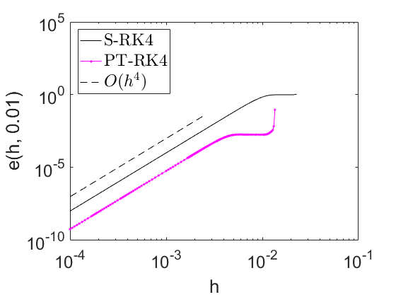
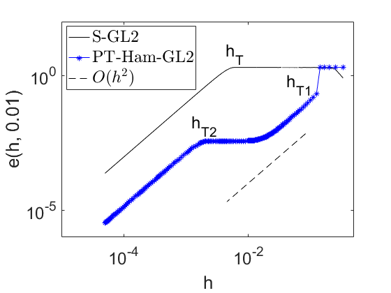
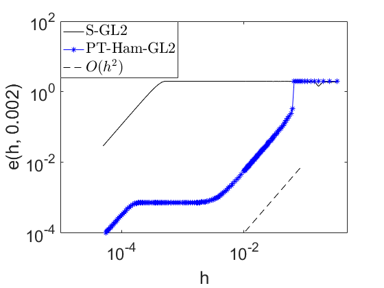
Fig. 5.2 compares the performance of different methods for this toy example. The numerical error is computed by

\mathsf{e}(h,\epsilon)=\max_{n\text{ s.t. }nh\in[0,T]}\|u_{n}-u(t_{n})\|_{2}

where $u$ denotes $\psi$ for the Schrödinger dynamics, $\varphi$ for the PT dynamics and $(q,p)$ for the Hamiltonian systems, respectively.

We first consider the explicit numerical methods. Fig. 2(a) and 2(b) give a comparison between S-RK4 and PT-RK4. Not surprisingly, as an explicit method, RK4 is numerically unstable for large time steps under both cases, and achieves fourth order convergence for small time steps. Furthermore, when $h$ is small enough, $\mathsf{e}(h,\epsilon)$ of the PT dynamics is smaller than that of the Schrödinger dynamics. Fig. 3(a) presents a study on how $\mathsf{e}(h,\epsilon)$ depends on $\epsilon$ , which reveals that by propagating the PT dynamics we gain one extra order of accuracy in terms of $\epsilon$ . This agrees with the theoretical results in Section 4.

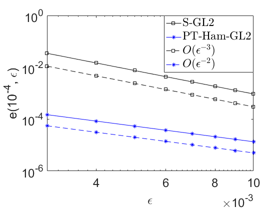
Next we test GL2 as an example of implicit symplectic methods applied to the Hamiltonian systems. Fig. 2(c) compares the numerical performances of S-GL2 and PT-Ham-GL2. For small $h$ , we observe a smaller error using the PT formulation, i.e. $\mathsf{e}(h,\epsilon)$ of S-GL2 is $\mathcal{O}(h^{2}/\epsilon^{3})$ and $\mathsf{e}(h,\epsilon)$ of PT-Ham-GL2 is $\mathcal{O}(h^{2}/\epsilon^{2})$ (see Fig. 3(b) for a study on the $\epsilon$ dependence). This verifies the estimate in Theorem 10. Despite that GL2 is a numerically stable scheme with a large time step, the step size of S-GL2 is constrained by the requirement of the accuracy, while the step size of PT-Ham-GL2 can be chosen to be considerably larger.

More specifically, let us define the “turning point” $h_{T}$ to be the largest time step size when a scheme starts to converge. Numerically for second order schemes the turning point can be computed as

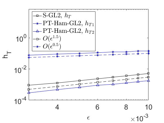
h_{T}=\arg\max\left\{h\in[h_{1},h_{2}]:\frac{\partial(\log\mathsf{e})}{\partial(\log h)}>1\right\}

where $[h_{1},h_{2}]$ is a suitable interval containing the convergence interval of interests. In Fig. 2(c) we mark the turning points in S-GL2 and PT-Ham-GL2, and study their dependence on $\epsilon$ in Fig. 4(a). For S-GL2, the convergence starts at $h_{T}=\mathcal{O}(\epsilon^{3/2})$ . For PT-Ham-GL2, a two-stage convergence behavior is observed. As $h$ decreases, the scheme first starts to converge with second order at a relatively large time step $h_{T1}=\mathcal{O}(\epsilon^{1/2})$ . This first stage ends at $h=\mathcal{O}(\epsilon)$ when $\mathsf{e}(h,\epsilon)$ reaches a plateau with its magnitude being $\mathcal{O}(\epsilon)$ (see Fig. 4(b)). Then the second-stage convergence starts at $h_{T2}=\mathcal{O}(\epsilon^{3/2})$ .

In the end we compare the schemes PT-Ham-GL2, PT-GL2 and PT-CN. Although we only justified the behavior of the global error for PT-Ham-GL2, numerical results in Fig. 5(a) and 5(b) indicate that there is no essential difference among these methods in practice.

5.1.2 Beyond adiabatic regime

As the value of $\delta$ is reduced, the second eigenstate corresponding to $\lambda_{2}$ may contribute significantly to the wave function, which leads to the violation of the adiabatic regime.

Fig. 5.6 investigates the Schrödinger wave function and the PT wave function with $\epsilon=0.002,\delta=0.05$ . Fig. 6(a) and 6(b) compare the real parts of the Schrödinger wave function and the PT wave function. When $t<t_{0}=0.5$ , the system stays close to the adiabatic regime and the PT wave function is nearly flat. However, when $t>t_{0}$ , the PT wave function starts to oscillate as well. Fig. 6(c) shows an orthogonal decomposition of the PT wave function into two orthogonal eigenspaces. Fig. 6(d) shows the evolution of the probability that the eigenstate corresponding to $\lambda_{2}(t)$ is occupied, which can be computed as $|c_{2}|^{2}=|(\varphi(t),e_{2}(t))|^{2}$ and $e_{2}(t)$ is the normalized eigenstate of $H(t)$ corresponding to $\lambda_{2}(t)$ . These results confirm that the oscillatory behavior originates from the excited state corresponding to $\lambda_{2}$ .

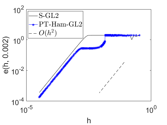
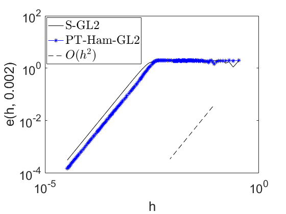
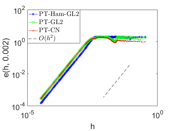
As discussed before, such oscillatory nature in the wave functions may increase the computational difficulty and require a smaller time step even for the PT dynamics. Fig. (5.7) compares $\mathsf{e}(h,\epsilon)$ for S-GL2, PT-Ham-GL2, PT-GL2 and PT-CN respectively. The results confirm that the PT dynamics is always more accurate than the Schrödinger dynamics using the same step size, but the gain becomes smaller as $\delta$ decreases.

5.2 Nonlinear Schrödinger equation in one dimension

Next we study the performance of the PT dynamics in a singularly perturbed nonlinear Schrödinger equation in one dimension.

\begin{split}\mathrm{i}\epsilon\partial_{t}\psi(x,t)&=-\frac{1}{2}\partial^{2}_{x}\psi(x,t)+V(x,t)\psi(x,t)+g|\psi(x,t)|^{2}\psi(x,t),\ \ x\in[0,L]\\ \psi(x,0)&=\psi_{0}(x)\\ \psi(0,t)&=\psi(L,t){.}\end{split}

(5.2)

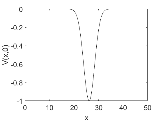
We set $L=50$ , and the external potential is chosen to be a time-dependent Gaussian function modeling a moving potential well (Fig. 5.8)

V(x,t)=-\exp(-0.1(x-R(t))^{2})

(5.3)

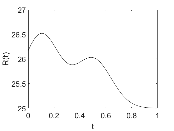
with a time-dependent center

R(t)=25+1.5\exp(-25(t-0.1)^{2})+\exp(-25(t-0.5)^{2}){.}

(5.4)

Note that $R(t)$ varies on the $\mathcal{O}(1)$ time scale.

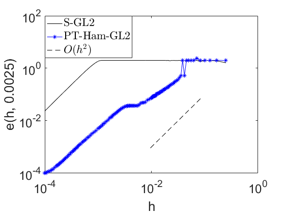
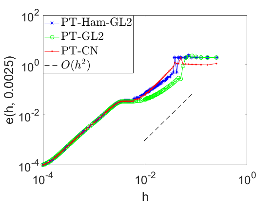
We use equidistant nodes $x_{k}=kh_{x}$ and the second-order finite difference scheme for spacial discretization, and we fix $h_{x}=0.025$ . Other parameters in this example are chosen to be $g=2.5,T=1,\epsilon=0.0025$ . For the choices of the parameters in the Anderson Mixing, the step length $\alpha=1$ , the mixing dimension is 20, and the tolerance is $10^{-8}$ . Fig. 5.9 compares $\mathsf{e}(h,\epsilon)$ of S-GL2, PT-Ham-GL2, PT-GL2 and PT-CN, and confirms the same numerical behavior as in the toy example.

Next we study the computational cost by comparing the total number of the Anderson mixing steps versus the numerical error $\mathsf{e}(h,\epsilon)$ up to $T=1$ . Fig. 5.10 clearly demonstrates that in order to achieve the same level of accuracy, all the methods propagating the PT dynamics, including PT-Ham-GL2, PT-GL2 and PT-CN, are much more efficient than S-GL2. This is valid across the entire range of the step sizes under study.

5.3 Time-dependent density functional theory in three dimension

As the last example, we demonstrate the performance of the PT dynamics for a benzene molecule driven by an ultrashort laser pulse using the time-dependent density functional theory (TDDFT). The TDDFT equations are

\mathrm{i}\partial_{t}\Psi(t)=H(t,P)\Psi(t),\quad P(t)=\Psi(t)\Psi^{*}(t),

(5.5)

and the corresponding PT-TDDFT equations are

\mathrm{i}\partial_{t}\Phi(t)=H(t,P)\Phi(t)-\Phi(t)\Phi^{*}(t)H(t,P)\Phi(t),\quad P(t)=\Phi(t)\Phi^{*}(t).

(5.6)

The number of wavefunctions $N$ is 15 for benzene example. Compared to the setup of singularly perturbed equations, here in the sense that the parameter $\epsilon$ is formally set to $1$ in TDDFT equations. However, as will be seen later, the PT dynamics can still result in significant computational advantage. The Hamiltonian takes the form

H(t,P)=-\frac{1}{2}\Delta+V_{\mathrm{ext}}(\mathbf{r},t)+V_{\mathrm{PP}}(\mathbf{r})+V_{\mathrm{Hxc}}[\rho(t)].

(5.7)

Here $V_{\mathrm{PP}}$ is the pseudopotential operator due to the electron-ion interaction, and we use the Optimized Norm-Conserving Vanderbilt (ONCV) pseudopotential [14] with a kinetic energy cutoff $E_{\mathrm{cut}}=30\text{ Hartree}$ . After spatial discretization, $V_{\mathrm{PP}}$ becomes a matrix independent of the time $t$ and the density matrix $P$ . $V_{\mathrm{Hxc}}$ is the sum of the Hartree and exchange-correlation potentials. We use the Perdew-Burke-Ernzerhof (PBE) [33] exchange correlation potential that depends on the electron density $\rho(t)=\mathrm{diag}[P(t)]$ . The external potential $V_{\text{ext}}(\mathbf{r},t)=\textbf{r}\cdot\textbf{E}(t)$ is given by a time-dependent electric field

\textbf{E}(t)=\hat{\textbf{k}}E_{\text{max}}\exp\Big[-\frac{(t-t_{0})^{2}}{2a^{2}}\Big]\sin[\omega(t-t_{0})]{,}

(5.8)

where $\hat{\textbf{k}}$ is a unit vector defining the polarization of the electric field. The parameters $a,t_{0},E_{\text{max}},\omega$ define the width, the initial position of the center, the maximum amplitude of the Gaussian envelope, and the frequency of the laser, respectively. In practice $\omega$ and $a$ are often determined by the wavelength $\lambda$ and the full width at half maximum (FWHM) pulse width [35], i.e. $\lambda\omega=2\pi c$ and $\text{FWHM}=2a\sqrt{2\log 2}$ , where $c$ is the speed of the light. In this example, the peak electric field $E_{\text{max}}$ is 1.0 eV/Å, occurring at $t_{0}=15.0$ fs. The FWHM pulse width is 6.0 fs, and the polarization of the laser field is aligned along the $x$ axis (the benzene molecule is in $x$ - $y$ plane, see Fig. 11(a)). We consider one relatively slow laser with wavelength 800 nm, and another faster laser with wavelength 250 nm, respectively (Fig. 5.11). The electron dynamics for the first laser is in the near adiabatic regime, where the system stays near the ground state after the active time interval of the laser, while the second laser drives electrons to excited states. We implement S-RK4 and PT-CN in the PWDFT package, and propagate TDDFT to $T=30.0$ fs. For the parameters in the Anderson mixing, the step length $\alpha$ is $0.2$ , the mixing dimension is 10, and the tolerance is $10^{-6}$ . We measure the accuracy using the dipole moment $\mathbf{D}(t):=\mathrm{Tr}[\mathbf{r}P(t)]$ , as well as the energy difference $E(t)-E(0)$ along the trajectory.

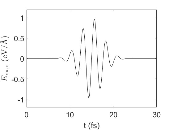
Figure 5.12 shows the numerical results for the 800 nm laser using S-RK4 with a step size 0.0005 fs and PT-CN with a step size 0.05 fs. In this case, the system stays near the ground state after the active time interval of the laser. After 25.0 fs, the total energy for S-RK4 only increases by $2.00\times 10^{-4}$ eV, and hence we may use the results from S-RK4 as our benchmark. We remark that S-RK4 becomes unstable at large time step sizes. Even when increasing the time step to be 0.001 fs, S-RK4 blows up within 100 time steps. We observe that PT-CN agrees perfectly with S-RK4 in terms of the dipole moment along the $x$ direction, and the total energy difference. After 25.0 fs, the total energy is nearly constant and only slightly increases by $2.44\times 10^{-4}$ eV compared to that of the initial state.

Since the computational cost of TDDFT calculations is mainly dominated by the cost of applying the Hamiltonian matrix to wave functions, we measure the numerical efficiency using the number of such matrix-vector multiplications. Although PT-CN requires more matrix-vector multiplications in each time step, the total number of matrix-vector multiplications is still significantly reduced due to the larger time step size, and PT-CN usually achieves a significant speedup. More specifically, in this case, during the time interval for which the laser is active (from 5.5 fs to 24.5 fs), the average number of matrix-vector multiplications in each PT-CN time step is 12.6, and the total number of matrix-vector multiplications in the simulation is 4798. On the other hand, the number of matrix-vector multiplications in each S-RK4 time step is 4, and the total number of matrix-vector multiplications during this period using time step 0.0005 fs is 152000. Hence the overall speedup of PT-CN over RK4 is $31.7$ .

Figure 5.13 shows the numerical results for the 250 nm laser. In this case, the laser carries more energy and hence a significant amount of electrons can reach the excited states. According to the S-RK4 benchmark, the total energy of the system increases by 0.5260 eV after 25.0 fs. Furthermore, the dipole moment along the $x$ direction oscillates more strongly due to the excitation. PT-CN needs to adopt a smaller time step size 0.005 fs, and still gives a very good approximation to the electron dynamics compared to S-RK4, For the dipole moment, PT-CN results match very well with S-RK4 benchmark during (Fig. 13(b)) and after (Fig. 13(c) and 13(d)) the active time interval of the laser. The total energy obtained by PT-CN matches very well with that in S-RK4 benchmark during the active interval and stays at a constant level with an average increase of 0.5340 eV by the end of the simulation (Fig. 13(e) and 13(f)). In this case, PT-CN slightly overestimates the total energy after the laser’s action by $7.96\times 10^{-3}$ eV.

For the computational costs within the period from 5.5 fs to 24.5 fs, the total number of matrix-vector multiplications is still 152000 for S-RK4. The average number of matrix-vector multiplications in each PT-CN time step is 7.5 due to the reduced step size, and the total number of matrix-vector multiplications is 28610. Therefore in this case PT-CN achieves 5.3 times speedup over S-RK4.

Method	h (fs)	AEI (eV)	AOE (eV)	MVM	Speedup
S-RK4	0.0005	0.5260	/	152000	/
PT-CN	0.005	0.5340	0.0080	28610	5.3
PT-CN	0.0065	0.5347	0.0087	22649	6.7
PT-CN	0.0075	0.5362	0.0102	21943	6.9
PT-CN	0.01	0.5435	0.0175	15817	9.6
PT-CN	0.02	0.5932	0.0672	12110	12.6

Table 1: Accuracy and efficiency of PT-CN for the electron dynamics with the 250 nm laser compared to S-RK4. The accuracy is measured using the average energy increase (AEI) after 25.0 fs and the average overestimated energy (AOE) after 25.0 fs. The efficiency is measured using the total number of matrix-vector multiplications (MVM) during the time interval from 5.5 fs to 24.5 fs, and the computational speedup.

We remark that even the electron dynamics is beyond the adiabatic regime, PT-CN can still be stable with a larger time step. Table 1 measures the accuracy of PT-CN with $h=$ 0.005 fs, 0.0065 fs, 0.0075 fs, 0.01 fs and 0.02 fs, respectively. We find that the number of matrix-vector multiplications systematically reduces as the step size increases. When the step size is 0.02 fs, the speed up over S-RK4 is $12.6$ , and this is at the expense of overestimating the energy by $0.0672$ eV after the active interval of the laser. Hence one can use PT-CN to quickly study the electron dynamics with a large time step, while this is not possible using an explicit scheme like S-RK4.

6 Conclusion

Quantum dynamics can be equivalently written in terms of the Schrödinger equation for the wave function, and the von Neumann equation for the density matrix. However, the Schrödinger dynamics may require a very small time step in numerical simulation due to the non-optimal gauge choice. In this paper, we propose to close this gap by identifying the optimal gauge choice, which is obtained from the parallel transport formulation. The solution of the resulting parallel transport (PT) dynamics can be significantly less oscillatory to that of the Schrödinger dynamics, especially in the near adiabatic regime. The PT dynamics is suitable to be combined with implicit time integrators, which allows the usage of large time steps even when the spectral radius of the Hamiltonian is large, and/or when $\epsilon$ is small. Although our global error analysis only applies to the Hamiltonian form of the PT dynamics with symplectic integrators and a relatively small time step, our numerical results indicate that the PT dynamics can be effectively discretized with more general numerical schemes and with much larger time steps. The mathematical understanding of the behavior with a large time step is our future work. Combining the PT dynamics with numerical schemes other than the Runge-Kutta methods and the linear multistep methods, as well as more detailed numerical studies of the PT dynamics for the time-dependent density functional theory calculations are also under progress.

Acknowledgments

This work was partially supported by the National Science Foundation under Grant No. 1450372, No. DMS-1652330 (D. A. and L. L.), and by the Department of Energy under Grant No. DE-SC0017867, No. DE-AC02-05CH11231 (L. L.). We thank the National Energy Research Scientific Computing (NERSC) center and the Berkeley Research Computing (BRC) program at the University of California, Berkeley for making computational resources available. We thank Stefano Baroni, Roberto Car, Weile Jia, Christian Lubich, and Lin-Wang Wang for helpful discussions.

References

[1] D. G. Anderson, Iterative procedures for nonlinear integral equations, J. Assoc. Comput. Mach., 12 (1965), pp. 547–560.
[2] J. E. Avron and A. Elgart, Adiabatic theorem without a gap condition, Communications in Mathematical Physics, 203 (1999), pp. 445–463.
[3] W. Bao, S. Jin, and P. A. Markowich, On time-splitting spectral approximations for the Schrödinger equation in the semiclassical regime, J. Comput. Phys., 175 (2002), pp. 487–524.
[4] F. A. Bornemann and C. Schütte, On the singular limit of the quantum-classical molecular dynamics model, J. Appl. Math., 59 (1999), pp. 1208–1224.
[5] H. Candy and W. Rozmus, A symplectic integration algorithm for seperate hamiltonian functions, J. Comput. Phys., 92 (1991), pp. 230–256.
[6] A. Castro, M. Marques, and A. Rubio, Propagators for the time-dependent Kohn-Sham equations, J. Chem. Phys., 121 (2004), pp. 3425–33.
[7] Z. Chen and E. Polizzi, Spectral-based propagation schemes for time-dependent quantum systems with application to carbon nanotubes, Phys. Rev. B, 82 (2010), p. 205410.
[8] D. Cohen, T. Jahnke, K. Lorenz, and C. Lubich, Numerical integrators for highly oscillatory hamiltonian systems: a review, in Analysis, modeling and simulation of multiscale problems, Springer, 2006, pp. 553–576.
[9] H. D. Cornean, D. Monaco, and S. Teufel, Wannier functions and z2 invariants in time-reversal symmetric topological insulators, Rev. Math. Phys., 29 (2017), p. 1730001.
[10] A. L. Fetter and J. D. Walecka, Quantum theory of many-particle systems, Courier Corp., 2003.
[11] E. Hairer, C. Lubich, and G. Wanner, Geometric numerical integration: structure-preserving algorithms for ordinary differential equations, Springer-Verlag Berlin Heidelberg, second ed., 2006.
[12] E. Hairer, S. P. Nørsett, and G. Wanner, Solving ordinary differential equation I: nonstiff problems, vol. 8, Springer, 1987.
[13] E. Hairer and G. Wanner, Solving ordinary differential equation II: stiff and differential-algebraic problems, vol. 8, Springer, 1991.
[14] D. R. Hamann, Optimized norm-conserving Vanderbilt pseudopotentials, Phys. Rev. B, 88 (2013), p. 085117.
[15] W. Hu, L. Lin, and C. Yang, DGDFT: A massively parallel method for large scale density functional theory calculations, J. Chem. Phys., 143 (2015), p. 124110.
[16] William Humphrey, Andrew Dalke, and Klaus Schulten, VMD – Visual Molecular Dynamics, J. Molec. Graphics, 14 (1996), pp. 33–38.
[17] A. Iserles, A first course in the numerical analysis of differential equations, no. 44, Cambridge Univ. Pr., 2009.
[18] T. Jahnke and C. Lubich, Numerical integrators for quantum dynamics close to the adiabatic limit, Numer. Math., 94 (2003), pp. 289–314.
[19] J. Jia and J. Huang, Krylov deferred correction accelerated method of lines transpose for parabolic problems, J. Comput. Phys., 227 (2008), pp. 1739–1753.
[20] C. F. Kammerer and A. Joye, Nonlinear quantum adiabatic approximation, arXiv:1906.11069, (2019).
[21] A.-K. Kassam and L. N. Trefethen, Fourth-order time-stepping for stiff PDEs, SIAM J. Sci. Comput., 26 (2005), pp. 1214–1233.
[22] T. Kato, On the adiabatic theorem of quantum mechanics, J. Phys. Soc. J. Jpn., 5 (1950), pp. 435–439.
[23] C. T. Kelley, Iterative methods for optimization, vol. 18, SIAM, 1999.
[24] O. Koch and C. Lubich, Dynamical low-rank approximation, SIAM J. Matrix Anal. Appl., 29 (2007), pp. 434–454.
[25] L. Lin, J. Lu, L. Ying, and W. E, Adaptive local basis set for Kohn-Sham density functional theory in a discontinuous Galerkin framework I: Total energy calculation, J. Comput. Phys., 231 (2012), pp. 2140–2154.
[26] L. Lin and C. Yang, Elliptic preconditioner for accelerating self consistent field iteration in Kohn-Sham density functional theory, SIAM J. Sci. Comp., 35 (2013), pp. S277–S298.
[27] C. Lubich, On splitting methods for Schrodinger-Poisson and cubic nonlinear Schrodinger equations, Math. Comp., 77 (2008), pp. 2141–2153.
[28] M. Nakahara, Geometry, topology and physics, CRC Press, 2003.
[29] G. Nenciu, Linear adiabatic theory. exponential estimates, Communications in Mathematical Physics, 152 (1993), pp. 479–496.
[30] P. Nettesheim, F. A.Bornemann, B. Schmidt, and C. Schütte, An explicit and symplectic integrator for quantum-classical molecular dynamics, Chem. Phys. Lett., 256 (1996), pp. 581–588.
[31] P. Nettesheim and C. Schütte, Numerical integrators for quantum-classical molecular dynamics, (1999), pp. 396–411.
[32] G. Onida, L. Reining, and A. Rubio, Electronic excitations: density-functional versus many-body Green’s-function approaches, Rev. Mod. Phys., 74 (2002), p. 601.
[33] J. P. Perdew, K. Burke, and M. Ernzerhof, Generalized gradient approximation made simple, Phys. Rev. Lett., 77 (1996), pp. 3865–3868.
[34] E. Runge and E. K .U. Gross, Density-functional theory for time-dependent systems, Phys. Rev. Lett., 52 (1984), p. 997.
[35] A. Russakoff, Y. Li, S. He, and K. Varga, Accuracy and computational efficiency of real-time subspace propagation schemes for the time-dependent density functional theory, J. Chem. Phys., 144 (2016), p. 204125.
[36] A. Schleife, E. W. Draeger, Y. Kanai, and A. A. Correa, Plane-wave pseudopotential implementation of explicit integrators for time-dependent Kohn-Sham equations in large-scale simulations, J. Chem. Phys., 137 (2012), p. 22A546.
[37] C. Sparber, Weakly nonlinear time-adiabatic theory, Ann. Henri Poincáre, 17 (2016), pp. 913–936.
[38] S. Teufel, Adiabatic perturbation theory in quantum dynamics, Springer-Verlag Berlin Heidelberg, first ed., 2003.
[39] Z. Wang, S.-S. Li, and L.-W. Wang, Efficient real-time time-dependent density functional theory method and its application to a collision of an ion with a 2D material, Phys. Rev. Lett., 114 (2015), pp. 1–5.