Scale-invariance as the cause of the superconducting dome in the cuprates

Understanding the physics of cuprate superconductors involves identifying the low-energy degrees of freedom responsible for the normal state’s anomalous features, such as $T$-linear resistivity, pseudogap, and Fermi arcs. In general, the electron Green function can be written as $G\left(k,\omega\right)=\left[\omega-\epsilon_{k}-\Sigma\left(\omega\right)\right]^{-1}$, where $\epsilon_{k}$ is the bare energy spectrum, and $\Sigma$ is the self-energy. Recent angle-resolved photoemission spectroscopy (ARPES) measurements [1] of the cuprates have revealed that the imaginary part of the electron self-energy has the scaling form

over a wide range of doping. The key parameter here is the scaling exponent $\alpha$, which varies from $\alpha=1$ in the overdoped Fermi-liquid state to $\alpha=\frac{1}{2}$ at optimal doping, and to $\alpha<\frac{1}{2}$ at underdoping. Other relevant parameters include a dimensionless coupling constant $\lambda\sim 0.5$, a high-energy scale $\omega_{N}\sim 0.5\mbox{ eV}$ to maintain dimensional consistency, and an impurity scattering term $\Gamma_{0}\sim 8\text{ to }35\mbox{ meV}$.

What is new here is that this scaling form persists over a wide range of doping, manifesting not just at a single point as traditional critical scenarios would suggest. Given the novelty of this scaling form, it is peculiar that the full consequences of this power-law scaling have not been explored previously. It is just this task that we perform here. We explore the consequences for 1) the Fermi velocity, 2) the effective mass, 3) the quasiparticle weight, and 4) the superconducting dome. All these quantities reveal truly unusual behaviors that are directly related to the power-law liquid’s unconventional scaling observed in the experiments.

Theoretically, mechanisms yielding non-Fermi-liquid scalings have been extensively studied [2, 3, 4, 5, 6, 7, 8, 9, 10, 11]. In a marginal Fermi liquid [2], a polarizability proportional to $\omega/T$ leads to $T$-linear resistivity, while a $d$-wave Pomeranchuk instability in two dimensions [3] yields self-energies with $\omega^{2/3}$ and $T^{2/3}$ dependence. In addition, similar behaviors can also be obtained by coupling quasiparticles with gauge bosons [4], Goldstone bosons [5], and critical bosons [6] near a quantum critical point [7]. Furthermore, strong coupling theories using the anti-de Sitter spacetime (AdS)/conformal field theory (CFT) correspondence [8] and Gutzwiller projection in hidden Fermi-liquid theory [9] also exhibit $T$-linear resistivity. In particular, the spectral functions calculated within the AdS/CFT formalism can also exhibit a range of power-law scaling when the scaling dimension of the boundary fermionic operator is tuned continuously [10, 11].

Given the interest in experimentally relevant self-energies for the cuprates, it is truly remarkable that the experimental consequences of the power-law liquid have not been explored until now. Specific to Eq. 1, since the scaling form is robust up to $0.1\mbox{ eV}$ and $250\mbox{ K}$ [1], we showed previously that such a behavior can originate from interactions between electrons and unparticles, a scale-invariant sector that naturally emerges due to strong correlations in the cuprates [12, 13]. Originally proposed as a scale-invariant sector within the standard model [14], unparticles can arise in the cuprates because any nontrivial infrared dynamics in a strongly correlated electron system is controlled by a critical fixed point. Consequently, scale invariance can be used to construct the form of the underlying propagator. This propagator which can acquire an anomalous dimension within the renormalization group approach is the unparticle propagator. Furthermore, in the context of AdS/CFT, one of us [15, 16] showed that a massive scalar field in the bulk is generally dual to a nonlocal operator (i.e., a fractional Laplacian) on the boundary. The propagator of these operators is of a power-law form, just like the unparticle propagator. These results indicate that unparticles should generically exist in a strongly coupled system.

In the context of the cuprates, unparticles have been proposed to explain the absence of Luttinger’s theorem in the pseudogap phase [17] using zeros in the Green function [18] and have also been found to yield unusual superconducting properties [17, 19, 20] and optical conductivity [21].

In particular, a power-law liquid can be obtained from interactions between electrons and unparticles [12, 13]. The propagator of fermionic unparticles can be written as $G_{u}\left(k,i\omega_{n}\right)=[i\omega_{n}-\epsilon^{u}_{k}]^{-1+d_{u}}$, where $d_{u}$ is the anomalous dimension and $\epsilon^{u}_{k}$ is the energy spectrum of unparticles. Due to the branch cut in the unparticle propagator, the scattering phase space for electron-unparticle interactions is nontrivially altered. Consequently, the electron self-energy due to such interactions scales with energy and temperature, with the scaling exponent $\alpha$ dependent on the anomalous dimension $d_{u}$ of the unparticle propagator as $d_{u}=\alpha-1$ [13].

In this paper, we study the superconducting $T_{c}$ of a power-law liquid. Within the BCS formalism, we show that the $T_{c}$ is non-monotonic with respect to $\alpha$, the self-energy scaling exponent. The $T_{c}$ peaks at $\alpha=\frac{1}{2}$, reproducing the cuprates’ superconducting dome. We attribute this behavior to the scaling form of the electron spectral function at low energies, where the scaling exponent is minimum at $\alpha=\frac{1}{2}$. Furthermore, we find that, due to strong renormalization of the spectral weights towards the Fermi level, the Fermi velocity vanishes and the effective mass diverges for $\alpha\leq\frac{1}{2}$, in agreement with earlier experimental observations [22, 23, 24]. Our results suggest that a power-law liquid contains physics central to understanding the cuprates.

The first obvious quantity to calculate is the real part of the electron self energy. This can be done directly from the Kramers-Kronig relationship:

Interested in only the low energy behavior, we integrate up to the high-energy scale $\omega_{N}$, assuming that the effects of $\Sigma^{\prime\prime}$ at higher energies are negligible. Also, for the integral to be analytically tractable, we omit the $T$-dependence in the self-energy. As detailed in App. A, we obtain

where $\!\,{}_{2}F_{1}\left(a,b;c;z\right)$ is the hypergeometric function. Illustrated in Fig. 1 (inset), this result strongly influences several low-energy behaviors of a power-law liquid. For notational simplicity, we measure energies in units of $\omega_{N}$. For concreteness, we consider a quadratic bare energy spectrum $\epsilon_{k}=k^{2}-k_{F}^{2}$ in two dimensions, with Fermi momentum $k_{F}=1/\sqrt{2}$. Since our focus is the $\alpha$-dependence of low-energy properties, we fix $\Gamma_{0}$ at a constant value of $0.01$.

The renormalized band $\epsilon_{k}^{\prime}$ is determined by $\epsilon_{k}^{\prime}-\epsilon_{k}-\Sigma^{\prime}\left(\epsilon_{k}^{\prime}\right)=0$. Fig. 1 shows that, close to the Fermi level, the bare dispersion is strongly renormalized towards the Fermi level for $\alpha<\frac{1}{2}$. This is quantified by the Fermi velocity $v_{F}$, which is renormalized by the quasiparticle residue $Z$ via $v_{F}^{\prime}=Zv_{F}$, where

A similar result was obtained in Ref. 1. The two cases arise due to the $\left|x\right|^{2\alpha}$ term in $\Sigma^{\prime}$. The quasiparticle residue $Z$ of a Fermi liquid quantifies how particle-like the system is, with unity denoting completely particle-like. The vanishing of the quasiparticle residue for $\alpha\leq\frac{1}{2}$ therefore reflects the absence of any particle-like behavior in a power-law liquid, indicative of the strong correlations in underdoped cuprates. A similar behavior also exists in an ultracold Fermi gas with strong interactions [25].

Shown in Fig. 2, the Fermi velocity $v_{F}$ vanishing for $\alpha\leq\frac{1}{2}$ quantifies the strong renormalization of the band towards the Fermi level. Experimentally, the Fermi velocity can be determined from the slope of the band close to, but not exactly at, the Fermi level. In Ref. 22, ARPES measurements of the nodal Fermi velocity within $7\mbox{ meV}$ of the Fermi level show that the Fermi velocity decreases monotonically with underdoping. This behavior is reproduced in Fig. 2, which shows that the power-law liquid’s velocity just below the Fermi level decreases with $\alpha$.

The vanishing Fermi velocity also implies that the effective mass $m^{*}=k_{F}/v_{F}^{\prime}$ diverges as $\left(\alpha-\frac{1}{2}\right)^{-1}$, as shown in Fig. 2. This behavior has been observed in the cuprates via quantum oscillations measurements [23, 24] and is attributed to a metal-insulator transition beneath the superconducting dome. Our results thus far are robust in the sense that they are independent of the values of $\Gamma_{0}$ and $\lambda$.

It is important to note that while ARPES measured the self-energy $\Sigma^{\prime\prime}$ over a limited energy range, the behavior of $\Sigma^{\prime\prime}$ at high energies is immaterial to our key result that the Fermi velocity $v_{F}$ vanishes when $\alpha\leq\frac{1}{2}$. This is because the vanishing of $v_{F}$ arises from the divergence of $d\Sigma^{\prime}/d\omega$ at $\omega=0$. From the form of the Kramers-Kronig relation, $\Sigma^{\prime\prime}$ at high energies has a finite contribution to $d\Sigma^{\prime}/d\omega|_{\omega=0}$ and so cannot affect the presence of the divergence.

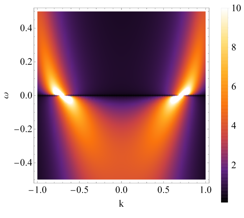
Next, the spectral function given by $-\text{Im}G$ is

where $N$ is a normalization constant dependent only on $\alpha$ ¹¹ 1 Due to how the self-energy $\Sigma^{\prime\prime}$ from Eq. 1 was obtained from ARPES momentum distribution curves, $N$ is momentum independent.. To make comparisons between different values of $\alpha$, we define $N$ such that the sum rule $\int_{-\omega_{n}}^{\omega_{n}}d\omega A\left(k=k_{F},\omega\right)=1$ is obeyed for all $\alpha$’s, where $\omega_{n}$ is a high-energy cutoff which we fix at $0.05\omega_{N}$. Fig. 3 illustrates the increased shifting and broadening of the spectral function as $\alpha$ decreases. This effect is also reflected in the density of states discussed in App. B. Finally, since the self-energy at the Fermi level is $\alpha$-independent, so is the Fermi momentum $k_{F}$, and the Fermi surface remains sharp even when $\alpha\leq\frac{1}{2}$. A sharply defined Fermi surface despite a vanishing quasiparticle residue represents a critical Fermi surface [27].

Next, we focus on the superconducting properties of a power-law liquid. We consider the simplest case of $s$-wave pairing symmetry with a constant pairing interaction $g$ within an energy range $\omega_{D}$. Within the BCS formalism, the superconducting $T_{c}$ is determined by the pairing instability equation [17]

From how the spectral function $A\left(k,\omega\right)$ is strongly renormalized towards the Fermi level for $\alpha\leq\frac{1}{2}$, we expect the superconducting $T_{c}$ to monotonically increase as $\alpha$ decreases. However, numerical solutions to the instability equation show that the superconducting $T_{c}$ is non-monotonic with respect to $\alpha$, peaking at $\alpha=\frac{1}{2}$. Shown in Fig. 4a is a power-law liquid reproducing the cuprates’ superconducting dome. This is the central result of this paper.

To understand the origin of the $T_{c}$’s $\alpha$-dependence, we consider the minimal BCS coupling $g_{\min}$ needed for superconductivity by setting $T_{c}=0$ in Eq. :

Fig. 4b shows that $g_{\min}$ is non-monotonic with respect to $\alpha$. In particular, the peak of $1/g_{\min}$ approaches $\alpha\approx\frac{1}{2}$ as the impurity term $\Gamma_{0}$ decreases. A similar behavior in fact appears in Fig. 4a where the peak $T_{c}$ approaches $\alpha=\frac{1}{2}$ as $g$ increases. When $g$ increases, superconductivity onsets in a higher temperature regime where the impurity term $\Gamma_{0}$ is less significant. This implies that as $\Gamma_{0}/T_{c}$ decreases, the peak $T_{c}$ approaches $\alpha=\frac{1}{2}$. These behaviors suggest a closer study of the $\Gamma_{0}=0$ case. Since solutions for $g_{\min}$ and $T_{c}$ at $\Gamma_{0}=0$ are numerically inaccessible, we proceed with a scaling argument.

Note that in Fig. 4b, small values ($\lesssim 0.002$) of $\Gamma_{0}$ are anomalous because of numerical uncertainties associated with convergence issues. It is for the same reason the desired results for $\Gamma_{0}=0$ are numerically inaccessible and require the following scaling argument.

When $\Gamma_{0}=0$, the spectral function close to the Fermi level ($\epsilon,\omega\rightarrow 0$) has the scaling form

The two cases arise from the competition between linear and nonlinear terms in the denominator. More concisely,

with the scaling exponent

This means that the spectral function’s scaling exponent $\xi\left(\alpha\right)$ has a minimum value of $-1$ at $\alpha=\frac{1}{2}$, as illustrated by the orange dashed line in Fig. 5. This result can also be verified numerically for $\Gamma_{0}=0$. First, the linearity of the log-log plot in the inset illustrates that the spectral function $A(k=k_{F},\omega)$ from Eq. 5 indeed has a scaling form for the energy range shown. Then, the scaling exponent obtained by numerical fits is indicated by the blue solid line in the main figure. The solid line from numerical fits slightly differs from the analytic results because the latter is obtained in the $\omega\rightarrow 0$ limit while the former is a fit over a finite energy window. One can easily verify that the numerical results approach the analytic ones if the energy window is taken to the same limit. More precisely, the blue numerical result at $\alpha=0.5$ approaches $-1$ in the limit $\omega\rightarrow 0$, in agreement with the analytic results.

Now, consider the integral for $g_{\min}$ in spherical coordinates $\left(r,\theta,\phi\right)$ near the origin:

Simply counting the powers of $r$ reveals that the integral diverges logarithmically at $\alpha=\frac{1}{2}$ . This implies that $g_{\min}\sim 0$ at $\alpha=\frac{1}{2}$, and a power-law liquid becomes most susceptible to superconductivity. Therefore, the superconducting dome in Fig. 4a can fundamentally be attributed to the scaling form of the spectral function.

We conclude with five pertinent points. First, we have used an $\alpha$-independent impurity scattering term $\Gamma_{0}$ in our calculations. Experimentally, $\Gamma_{0}$ in fact varies with $\alpha$ [1]. It is minimum ($\sim 8\mbox{ meV}$) at optimal doping and about four (two) times larger with underdoping (overdoping). Since impurity scattering opposes superconductivity, one can show that such a $\Gamma_{0}$ produces a narrower superconducting dome.

Second, let us reiterate a subtle point about Fig. 4a. According to the scaling argument, the $T_{c}$ peaks at $\alpha=\frac{1}{2}$ because of the low-energy scaling of the spectral function when $\Gamma_{0}=0$. Since $\Gamma_{0}$ is nonzero in Fig. 4a, the peak $T_{c}$ naturally deviates from $\alpha=\frac{1}{2}$. More precisely, notice that the deviation increases as $g$ decreases, for a fixed $\Gamma_{0}$. What is happening is that when $g$ decreases, superconductivity onsets in a lower temperature regime where the impurity term $\Gamma_{0}$ is more significant, resulting in a larger deviation from $\alpha=\frac{1}{2}$. Nevertheless, the results in Fig. 4a require $g$ to be sufficiently small. This is so that the resulting $T_{c}$ is low enough for the physics to be dominated by the low-energy scaling behavior of the spectral function $A$ given by Eq. 9. For sufficiently large $g$, the scaling argument for the superconducting dome in the preceding section is inapplicable, and indeed we find that the $T_{c}$ becomes monotonic, and the superconducting dome vanishes.

Third, superconducting domes in other unconventional superconductors have been attributed to various mechanisms [28]. In $\text{Sr}\text{Ti}\text{O}_{3}$, screening effects [29], longitudinal optical phonons [30], and a quantum critical point [31] have been suggested. Quasiparticle-phonon interactions in dichalcogenides [32, 33] and a Mott transition in organic superconductors [34] have also been proposed. For the cuprates, self-energy effects near the charge-density wave instability have been theorized [35]. Our present results show that the power-law self-energy inferred from ARPES experiments can produce the superconducting dome.

Fourth, the self-energy in Eq. 1 was obtained from measurements along the nodal lines of the cuprates. It is true that an accurate calculation of the superconducting $T_{c}$ would require measurements over the entire Brillouin zone. However, this was not our goal. Our goal was to study the implications of the novel self-energy revealed by the ARPES measurements. Given the lack of experimental data for the non-nodal regions, the most direct approach naturally assumes that the scaling form is applicable throughout the whole Brillouin zone. Doing otherwise would unnecessarily obfuscate the results which demonstrate a novel mechanism for obtaining the cuprates’ superconducting dome. It is worth highlighting that, recently, similar measurements found that the antinodal self-energies are a few times larger [36]. Furthermore, as the superconducting gap develops, $\Sigma^{\prime\prime}$ markedly decreases while $\Sigma^{\prime}$ increases. This implies that correlations in the normal state are converted into a strongly renormalized coherent state below $T_{c}$. It will be interesting to incorporate these effects into the power-law liquid model in a future work.

Fifth, our superconducting $T_{c}$ calculations adopt the simplest case of $s$-wave gap symmetry, in contrast to the $d$-wave symmetry known in the cuprates. As presented in Sec. III, the key feature of our results arises from the scaling form of the spectral function given by Eq. 9. This scaling form is intrinsic to the power-law self-energy, independent of the superconducting gap symmetry. What a $d$-wave symmetry modifies is the momentum dependence in the pairing instability equation in Eq. ; the form of the equation’s dependence on the spectral function would remain unchanged. Therefore, our results are applicable even in the $d$-wave cuprates.

In conclusion, we studied the superconducting $T_{c}$ of a power-law liquid, an unconventional state of matter revealed in superconducting cuprates by recent ARPES measurements [1]. The imaginary part of the electron self-energy has the scaling form $\left(\omega^{2}+\pi^{2}T^{2}\right)^{\alpha}$, where the scaling exponent $\alpha$ varies from $\alpha\lesssim 1$ at overdoping to $\alpha\sim\frac{1}{2}$ at optimal doping, and to $\alpha\lesssim\frac{1}{2}$ at underdoping. We found that strong renormalization of the spectral weights results in a vanishing Fermi velocity and diverging effective mass for $\alpha\leq\frac{1}{2}$, in agreement with earlier experimental observations [22, 23, 24]. Within a BCS formalism, we found that the superconducting $T_{c}$ is non-monotonic with respect to $\alpha$. The $T_{c}$ peaks at around $\alpha\sim\frac{1}{2}$, reproducing the cuprates’ superconducting dome. We attribute this behavior to the low-energy scaling form of the spectral function, where the scaling exponent is minimum at $\alpha=\frac{1}{2}$. Our results suggest that a power-law liquid contains physics central to understanding cuprate superconductors.

References

- [1] T. J. Reber, X. Zhou, N. C. Plumb, S. Parham, J. A. Waugh, Y. Cao, Z. Sun, H. Li, Q. Wang, J. S. Wen, Z. J. Xu, G. Gu, Y. Yoshida, H. Eisaki, G. B. Arnold, and D. S. Dessau, Arxiv Prepr. , 01611 (2015), arXiv:1509.01611 .
- [2] C. M. Varma, P. B. Littlewood, S. Schmitt-Rink, E. Abrahams, and A. E. Ruckenstein, Phys. Rev. Lett. 63, 1996 (1989).
- [3] W. Metzner, D. Rohe, and S. Andergassen, Phys. Rev. Lett. 91, 066402 (2003).
- [4] S.-S. Lee, Phys. Rev. B 80, 165102 (2009), arXiv:0905.4532 .
- [5] H. Watanabe and A. Vishwanath, Proc. Natl. Acad. Sci. 111, 16314 (2014), arXiv:1404.3728 .
- [6] a. L. Fitzpatrick, S. Kachru, J. Kaplan, and S. Raghu, Phys. Rev. B 89, 165114 (2014), arXiv:1312.3321 .
- [7] S. Sachdev, Quantum Phase Transitions:, 2nd ed. (Cambridge University Press, Cambridge, 2011).
- [8] T. Faulkner, N. Iqbal, H. Liu, J. McGreevy, and D. Vegh, Science (80-. ). 329, 1043 (2010a).
- [9] P. A. Casey and P. W. Anderson, Phys. Rev. Lett. 106, 097002 (2011), arXiv:1101.3609v1 .
- [10] T. Faulkner, G. T. Horowitz, J. McGreevy, M. M. Roberts, and D. Veghc, J. High Energy Phys. 2010 (2010b), 10.1007/JHEP03(2010)121s, arXiv:0911.3402 .
- [11] J. Zaanen, Y. Liu, Y. W. Sun, and K. Schalm, Holographic Duality in Condensed Matter Physics (Cambridge University Press, 2015).
- [12] K. Limtragool, C. Setty, Z. Leong, and P. W. Phillips, Phys. Rev. B 94, 235121 (2016).
- [13] Z. Leong, C. Setty, K. Limtragool, and P. W. Phillips, Phys. Rev. B 96, 205101 (2017), arXiv:1705.07130 .
- [14] H. Georgi, Phys. Rev. Lett. 98, 221601 (2007), arXiv:0703260 [hep-ph] .
- [15] G. La Nave and P. W. Phillips, Phys. Rev. D 94, 126018 (2016), arXiv:1605.07525 .
- [16] G. La Nave and P. Phillips, (2017), arXiv:1702.00038 .
- [17] P. W. Phillips, B. W. Langley, and J. A. Hutasoit, Phys. Rev. B 88, 115129 (2013), arXiv:1305.0006 .
- [18] K. B. Dave, P. W. Phillips, and C. L. Kane, Phys. Rev. Lett. 110, 090403 (2013), arXiv:1207.4201 .
- [19] J. P. F. LeBlanc and A. G. Grushin, New J. Phys. 17, 1 (2015), arXiv:1407.8492 .
- [20] A. Karch, K. Limtragool, and P. W. Phillips, J. High Energy Phys. 2016, 175 (2016), arXiv:1511.02868 .
- [21] K. Limtragool and P. Phillips, Phys. Rev. B 92, 155128 (2015), arXiv:arXiv:1506.00649v4 .
- [22] I. M. Vishik, W. S. Lee, F. Schmitt, B. Moritz, T. Sasagawa, S. Uchida, K. Fujita, S. Ishida, C. Zhang, T. P. Devereaux, and Z. X. Shen, Phys. Rev. Lett. 104, 207002 (2010).
- [23] S. E. Sebastian, N. Harrison, M. M. Altarawneh, C. H. Mielke, R. Liang, D. A. Bonn, W. N. Hardy, and G. G. Lonzarich, Proc. Natl. Acad. Sci. 107, 6175 (2009), arXiv:0910.2359 .
- [24] J. Singleton, C. De La Cruz, R. D. McDonald, S. Li, M. Altarawneh, P. Goddard, I. Franke, D. Rickel, C. H. Mielke, X. Yao, and P. Dai, Phys. Rev. Lett. 104, 5 (2010), arXiv:0911.2745 .
- [25] Y. Sagi, T. E. Drake, R. Paudel, R. Chapurin, and D. S. Jin, Phys. Rev. Lett. 114, 075301 (2015), arXiv:1409.4743 .
- [26] Due to how the self-energy from Eq. 1 was obtained from ARPES momentum distribution curves, is momentum independent.
- [27] T. Senthil, Phys. Rev. B 78, 035103 (2008), arXiv:0803.4009 .
- [28] T. Das and C. Panagopoulos, New J. Phys. 18, 103033 (2016).
- [29] C. S. Koonce, M. L. Cohen, J. F. Schooley, W. R. Hosler, and E. R. Pfeiffer, Phys. Rev. 163, 380 (1967).
- [30] L. P. Gor’kov, Proc. Natl. Acad. Sci. 113, 4646 (2016), arXiv:1508.00529 .
- [31] J. M. Edge, Y. Kedem, U. Aschauer, N. A. Spaldin, and A. V. Balatsky, Phys. Rev. Lett. 115, 247002 (2015), arXiv:1507.08275 .
- [32] T. Das and K. Dolui, Phys. Rev. B 91, 094510 (2015), arXiv:1411.3096 .
- [33] M. Calandra and F. Mauri, Phys. Rev. Lett. 106, 196406 (2011).
- [34] C.-D. Hébert, P. Sémon, and A.-M. S. Tremblay, Phys. Rev. B 92, 195112 (2015), arXiv:arXiv:1509.07086v1 .
- [35] G. Buzon, A. Foussats, M. Bejas, and A. Greco, Phys. Rev. B 89, 024516 (2014).
- [36] H. Li, X. Zhou, S. Parham, T. J. Reber, H. Berger, G. B. Arnold, and D. S. Dessau, Nat. Commun. 9, 26 (2018).
- [37] DLMF, “NIST Digital Library of Mathematical Functions,” http://dlmf.nist.gov/, Release 1.0.17 of 2017-12-22, f. W. J. Olver, A. B. Olde Daalhuis, D. W. Lozier, B. I. Schneider, R. F. Boisvert, C. W. Clark, B. R. Miller and B. V. Saunders, eds.