Electron drift properties in high pressure gaseous xenon

Electron drift properties, particularly drift velocity and diffusion, play a major role in the TPC tracking performance. In particular, the measurement of electron drift properties is of special relevance for the NEXT-White detector and its immediate successor, the NEXT-100 apparatus. Both are part of the NEXT program, which is developing the technology of high-pressure xenon gas TPCs with electroluminescent amplification (HPXe-EL) for neutrinoless double beta decay searches [1, 2, 3, 4, 5]. The first phase of NEXT exploited two prototypes, DEMO and DBDM, which demonstrated the robustness of the technology, its excellent energy resolution and its particle-tracking capabilities [6, 7, 8, 9]. The NEXT-White¹¹ 1 Named after Prof. James White, our late mentor and friend. detector implements the second phase of the program. NEXT-White has been running successfully since December 2016 at the Canfranc Underground Laboratory (LSC). Its purpose is to validate the HPXe-EL technology in a large-scale radiopure detector. NEXT-White is a $\sim$1:2 model of NEXT-100, a 100 kg HPXe-EL detector, which is foreseen to start operations in 2019.

The NEXT-White detector started operations at the LSC late in 2016. After a short engineering run (Run I) in November-December 2016, the detector was operated continuously between March and December 2017 (Run II). This paper presents the measurement of drift parameters (drift velocity, longitudinal diffusion and transverse diffusion) for xenon at high pressure obtained during Run II. The measurements are inferred from calibration data obtained using a rubidium source (${}^{83}\mathrm{Rb}$) which provides a copious sample of krypton (${}^{83m}\mathrm{Kr}$) decays.

Electron transport properties in xenon gas have mostly been measured at low pressures [10, 11, 12, 13, 14, 15], usually not higher than atmospheric pressure with few exceptions at high pressure [16, 17]. In this regard, the NEXT Collaboration previously measured the drift velocity and the longitudinal diffusion at 10 bar in several prototypes [8, 18, 19]. However, transverse diffusion was not determined in the NEXT prototypes. In addition, measurements of the diffusion coefficients have recently been obtained by Kusano et al. [20] at pressures ranging from $1.7\text{\,}\mathrm{b}\mathrm{a}\mathrm{r}50\text{\,}\mathrm{b}\mathrm{a}\mathrm{r}$ and for reduced fields from $6\text{\,}\mathrm{V}\text{\,}{\mathrm{cm}}^{-1}\text{\,}{\mathrm{bar}}^{-1}45\text{\,}\mathrm{V}\text{\,}{\mathrm{cm}}^{-1}\text{\,}{\mathrm{bar}}^{-1}$. Despite 10 bar being rather far from the critical point of xenon at around 300 K (58 bar), those authors observed a strong deviation from the values expected from density-scalings, that remains unconfirmed. In order to reassess the situation, we provide here a simultaneous measurement of the three main transport observables in the range $20\text{\,}\mathrm{V}\text{\,}{\mathrm{cm}}^{-1}\text{\,}{\mathrm{bar}}^{-1}60\text{\,}\mathrm{V}\text{\,}{\mathrm{cm}}^{-1}\text{\,}{\mathrm{bar}}^{-1}$ for pressures of $7.2\text{\,}\mathrm{bar}$ and $9.1\text{\,}\mathrm{bar}$.

The paper is organized as follows: section 2 presents the principle of operation of a HPXe-EL TPC and the effect of diffusion in track reconstruction, the main features of the NEXT-White detector are summarized in section 3, the experimental setup is described in 4, the data selection in section 5, the measurement of the drift velocity is explained in section 6, the measurement of both longitudinal and transverse diffusion in section 7 and, finally, conclusions are presented in section 8

As discussed in [21], an HPXe-EL TPC is an optical TPC, where both the primary scintillation ($S_{1}$) and the ionization produce a light signal. In NEXT, the light is detected by two independent sensor planes located behind the anode and cathode. The energy of the event is measured by integrating the amplified EL signal ($S_{2}$) with a plane of photomultipliers (PMTs). This energy plane also records the $S_{1}$ signal which triggers the start-of-event ($t_{0}$).

Electroluminescent light provides tracking as well, since it is detected a few mm away from production at the anode plane via a denser array of silicon photomultipliers (SiPMs), which constitute the tracking plane. As $S_{2}$ light is produced in the EL region, near the sensors, $(x,y)$ information transverse to the drift direction can be extracted from the SiPM response. The longitudinal (or $z$) position of the event is inferred from the time difference between the $S_{1}$ and $S_{2}$ signals (i.e. the drift time). The drift time will depend on the velocity of the electrons under the influence of an electric field, the so-called drift velocity. Therefore, knowledge of the drift velocity is essential to correctly establish the $z$ position of the events.

In NEXT-White (and NEXT-100), the $(x,y)$ information comes directly from the light produced by the ionization electrons as they cross the EL gap, after drifting through the TPC active volume. As electrons travel through gas they diffuse, smearing the electron cloud produced by the interacting particle. As a result, the charge distribution arriving at the EL will be spread out.

In pure xenon, diffusion is large and affects tracking reconstruction. The effect is qualitatively illustrated in figure 1. A simulated neutrinoless double beta decay ($\beta\beta 0\nu$) track from ${}^{136}\rm Xe$ ($2458\text{\,}\mathrm{keV}$ deposited energy) interacting in xenon gas at $15\text{\,}\mathrm{bar}$ is shown on the left panel of the figure. On the right panel, the same track is imaged after a $40\text{\,}\mathrm{c}\mathrm{m}$ drift distance, assuming the known diffusion parameters at that pressure, i.e. $\sim$$0.3\ \textrm{mm}/\sqrt{\textrm{cm}}$ and $\sim$$1\ \textrm{mm}/\sqrt{\textrm{cm}}$ for the longitudinal and transverse diffusion, respectively. Although the main feature needed to identify the track as two electrons (i.e. the two high-energy depositions at the track end points) can still be discerned, the picture is blurred due to the spreading of the ionization electrons, resulting in loss of information of the particle path.

The large diffusion characteristic of pure xenon can be mitigated by using a xenon mixture rather than pure xenon. A number of such mixtures showing promising results have been studied by the NEXT collaboration [22, 23]. In this work we focus instead in a precise measurement of the drift parameters in pure xenon.

The NEXT-White detector has been thoroughly described elsewhere [21] and only a brief summary of its main features is offered here. It has three main subsystems, the TPC, the energy plane and the tracking plane. Table 1 shows the main parameters of the TPC. The energy plane is instrumented with $12$ Hamamatsu R11410-10 PMTs located $130\text{\,}\mathrm{mm}$ behind the cathode, providing a coverage of 31%. The tracking plane is instrumented with $1792$ SiPMs SensL series-C distributed in a square grid at a pitch of $10\text{\,}\mathrm{mm}$. An ultra-pure $60\text{\,}\mathrm{mm}$-thick copper shell (ICS) acts as a shield in the barrel region. The tracking plane and the energy plane are supported by $120\text{\,}\mathrm{mm}$-thick pure copper plates.

The detector operates inside a pressure vessel fabricated with a radiopure titanium alloy (316Ti) surrounded by a lead shield. Since a long electron lifetime is a must, xenon circulates in a gas system where it is continuously purified. The whole setup sits on top of a tramex platform elevated over the ground in HALL-A of LSC.

We refer to [26] for a detailed description of the data selection and event reconstruction. The detector triggers on the krypton $S_{2}$ signals using the two central PMTs of the energy plane. The recorded data are PMT and SiPM waveforms. As described in [21], the PMT waveforms show a negative swing due to the effect of the front-end electronics. The first step in the processing is to apply a deconvolution algorithm [21, 27], to the negative-swing, arbitrary-baseline, uncalibrated raw-waveforms (RWFs), to produce positive-only, zero-baseline, calibrated waveforms (CWFs). Figure 3 shows the CWF waveform corresponding to the sum of the PMTs in the energy plane. The detector triggers in the $S_{2}$ signal, centered in the middle of the data acquisition window. The $S_{1}$ signal appears in the left of the waveform, indicating that the event has drifted most of the chamber

The first half of the CWF (i.e. drift time less than $620\text{\,}\mathrm{\SIUnitSymbolMicro s}$) is processed by a peak-finding algorithm tuned to find small signals. A single $S_{1}$ is identified in about half of the events. The second half of the CWF (i.e. drift time more than $620\text{\,}\mathrm{\SIUnitSymbolMicro s}$) is then processed by the same peak finding algorithm, this time tuned to find larger signals. Most of the time a single $S_{2}$ candidate is found. Only events with exactly one $S_{1}$ and one $S_{2}$ are accepted for the analysis. Furthermore, a positive signal in at least one sensor of the tracking plane for the same time window of the $S_{2}$ is required. A SiPM is considered to have signal if the total charge in that time window exceeds $5\text{\,}\mathrm{pes}$ (photoelectrons). This threshold was taken to reduce the impact of SiPM dark noise at the operational temperature of the detector.

Next, the position of the selected events is reconstructed. The $z$ coordinate of the events is computed multiplying the drift time (obtained as the difference between $S_{1}$ and $S_{2}$) by the drift velocity. The transverse coordinates $(x,y)$ of the event are obtained using the position and integrated charge of the SiPMs. Concretely, the $(x,y)$ position is computed as the barycenter, the charge-weighted position of the SiPMs.

Finally, additional selections are applied to further increase the purity of the ${}^{83m}\mathrm{Kr}$ dataset. First, a $150\text{\,}\mathrm{mm}$ radial cut is applied to select a fiducial region away from the edges of the chamber where solid angle effects and fringe fields are important. Second, an energy selection is made.

For the energy selection, the lifetime of each run is measured by fitting the distribution of $S_{2}$ energy as a function of the drift time, as illustrated in figure 4. The lifetime has to be measured for each run as it depends not only on the attachment but also on the drift field [28]:

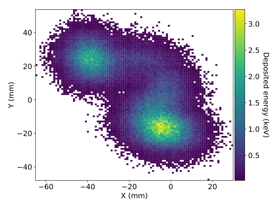
The $S_{2}$ energy corrected by attachment varies across the detector transverse dimensions due to the fact that the solid angle covered by the energy plane depends on the position of the event. Therefore, events have to be selected accordingly, as shown on figure 6. After all selections, around 23% of the triggered events remain. For more details on the technique, the energy calibration of the chamber using ${}^{83m}\mathrm{Kr}$ decays is fully described in [KRYPTON].

The drift velocity can be obtained by measuring the drift time for a known distance. In NEXT, the reference inside the chamber is the cathode plane, as its position is well measured. Since the cathode is the farthest $z$ from the EL region, the maximum drift time will correspond to that position, $Z_{cath}$. Consequently, the drift velocity is immediately given by:

However, a small correction has to be added to equation 6.1 to also consider the track time of the electrons crossing the EL region. We define the time positions of the $S_{2}$ and $S_{1}$ signals as those of the waveform’s time bin with maximum energy. Given the point-like nature of the events considered, the electron cloud arriving at the EL will follow a gaussian distribution due to diffusion. Since $S_{2}$ scintillation takes place uniformly during the electron cloud transit time throughout the EL region, the resulting $S_{2}$ signal can be seen approximately as a convolution with a square function, whose time duration equals the electron transit time ($t_{EL}$). Consequently, the signal peaking time is expected to be shifted by $t_{EL/2}$.

A Magboltz simulation of the drift field at the operational EL voltage ($7.0\text{\,}\mathrm{kV}$ at $7.2\text{\,}\mathrm{bar}$ and $8.5\text{\,}\mathrm{kV}$ at $9.1\text{\,}\mathrm{bar}$) has been done to estimate the travel time through the EL gap. Doing this, an EL crossing-velocity of $3.72\pm\pm 0.03\text{\,}\mathrm{mm}\text{\,}{\mathrm{\SIUnitSymbolMicro s}}^{-1}$ ($3.52\pm\pm 0.03\text{\,}\mathrm{mm}\text{\,}{\mathrm{\SIUnitSymbolMicro s}}^{-1}$) was obtained for the $7.2\text{\,}\mathrm{bar}$ ( $9.1\text{\,}\mathrm{bar}$) data. The EL gap in NEXT-White is $6\text{\,}\mathrm{mm}$  therefore the time it takes to cross half of that distance is $t_{EL/2}$ = $0.806\pm\pm 0.006\text{\,}\mathrm{\SIUnitSymbolMicro s}$ ($0.852\pm\pm 0.008\text{\,}\mathrm{\SIUnitSymbolMicro s}$).

On the other hand, the distance between cathode and gate is well known and measured to be $Z_{cath}$ = $530.3\pm\pm 2\text{\,}\mathrm{mm}$ and equation 6.1 results in:

The maximum drift time is obtained from the end-point of the drift time distribution, as shown in figure 7. The number of events, $N$, near the maximum drift time is fitted to a logistic function:

where $A$ is a constant that accounts for the height of the distribution, $B$ is related with the number of residual events after the steep drop of the function; $k$ is related with the steepness of the curve and $t_{max}$ corresponds to the drift time coordinate at half-height. The parameter $t_{max}$ gives the distribution end-point and the maximum drift time.

As a cross-check, Monte Carlo data has been generated with a drift velocity of $1\text{\,}\mathrm{mm}\text{\,}{\mathrm{\SIUnitSymbolMicro s}}^{-1}$. The fit to the simulated data, showed in figure 7, yields a drift velocity for the simulated data of $999.79\pm 0.05\ \textrm{(stat.)}\ \pm 1.88\ \textrm{(sys.)}\text{\,}\mathrm{\SIUnitSymbolMicro m}\text{\,}{\mathrm{\SIUnitSymbolMicro s}}^{-1}$. The central value differs by only 0.21 $\cdot$ 10^-3 from the value used for the simulation. This is well below the systematic error considered, of order 0.4%, which comes from the uncertainty in $Z_{cath}$, $t_{EL/2}$ and $t_{max}$.

In simulated data the uncertainty of the two first parameters is zero but that is not the case for the latter one, $t_{max}$. The uncertainty on $t_{max}$ has been considered to be equal to the time resolution of the detector, $1\text{\,}\mathrm{\SIUnitSymbolMicro s}$. Since the systematic error is at least an order of magnitude higher than the difference between measurement and simulation, we conclude that the analysis method does not add significant uncertainties to the result.

The drift velocities for the considered drift field conditions are shown in figure 8, where they are also compared with Magboltz simulation results. For the Run II standard conditions the result of the fit corresponds to a drift velocity of $967.99\pm 0.17\ \textrm{(stat.)}\ \pm 4.06\ \textrm{(sys.)}\text{\,}\mathrm{\SIUnitSymbolMicro m}\text{\,}{\mathrm{\SIUnitSymbolMicro s}}^{-1}$. A similar value was obtained in an independent analysis using alpha events in taken with NEXT-White during the Run II [29].The simulations have been run at 1 bar for each considered reduced drift field. The results of the $7.2\text{\,}\mathrm{bar}$ and $9.1\text{\,}\mathrm{bar}$ data match very well and show a smooth trend. This validates the usefulness of the reduced drift field as a quantity to be used to quote drift velocity results. In this way, results can be easily extrapolated to other operating pressures.

Our drift velocity results are systematically slightly higher than Magboltz predictions by a mean value of 1.2%, with the maximum deviation being 1.8% and the minimum 0.4%. This small discrepancy between Magboltz simulations and our results is also present in previous measurements of the NEXT Collaboration [18, 19], also shown in the figure, and could be due to the fact that the drift field is no longer uniform near the cathode mesh as it highly increases.

Diffusion of electrons drifting in gas due to the effect of an electric field follows a gaussian distribution whose standard deviation (RMS), $\sigma_{L,T}$, is defined by:

where $D_{L,T}$ is the longitudinal (L) or transverse (T) diffusion coefficient to be extracted, $\sigma_{0_{L,T}}$ is a free parameter of the fit that accounts for any additional spread, and $t_{drift}$ is the drift time of the events. As before, $t_{drift}$ is the measured drift time $t_{S2}-t_{S1}$ minus half of the transit time inside the EL region, $t_{EL/2}$. The spread $\sigma_{L,T}$ in equation 7.1 is given in length units, so it follows that $D_{L,T}$ is usually expressed in cm² $\cdot$ s^-1 units.

Following equation 7.1, a linear fit to the dependence of the squared spread with drift time is sufficient to obtain $D_{L,T}$.

A high precision characterization of different electron transport properties for xenon gas at high pressure has been presented in this work. Concretely, drift velocity, longitudinal diffusion and transverse diffusion have all been measured simultaneously, for the first time, using the same experimental setup. The analysis uses ${}^{83m}\mathrm{Kr}$ calibration data taken in the NEXT-White (NEW) detector at the Laboratorio Subterráneo de Canfranc (LSC) between September and October 2017, during Run II of the detector.

A study of the transport parameters dependence with reduced drift field has been done for two different gas pressures, $7.2\text{\,}\mathrm{bar}$ and $9.1\text{\,}\mathrm{bar}$. The results, after applying density scalings, are compatible, within 5% in most cases, with Magboltz simulations of pure xenon carried out at 1 bar and in the same reduced drift field conditions. In the drift velocity case, the average deviation between Magboltz and our results is of 1.2%, with a maximum deviation of 1.8%. The measured longitudinal diffusion shows an average deviation of 3.5%, while the maximum deviation is 6.6%. Finally, the mean deviation observed in the transverse diffusion is of 3.1%, with a maximum of 7.6%.

As can be seen in figure 17, the results are compatible with previous experimental measurements carried out at different pressures [10, 11, 16, 12, 20, 13, 17, 14, 15]. This level of agreement shows that pressure scaling of the diffusion parameters can be trusted for these operating pressures, suggesting that the role of dimers and higher order xenon clusters in electron transport is still minor at pressures up to $\sim$10 bar, at least. Therefore, we are unable to reproduce the results obtained in [20], where the reduced longitudinal diffusion coefficients showed a dependence with pressure when working in the same reduce field range studied here.

With regard to the implications of this result for the NEXT experiment, the measured longitudinal diffusion applicable to most of the 2017 NEXT-White calibration campaign is $318.9\pm 1.8\ \textrm{(stat.)}\ \pm 20.1\ \textrm{(sys.)}\ \micro\textrm{m}/\sqrt{\textrm{cm}}$, while the transverse diffusion value is $1279\pm 3\ \textrm{(stat.)}\ \pm 40\ \textrm{(sys.)}\ \micro\textrm{m}/\sqrt{\textrm{cm}}$. The NEXT collaboration will work at a minimum of $10\text{\,}\mathrm{bar}$ for the upcoming physics runs. This pressure implies a longitudinal diffusion of $267.3\pm 1.5\ \textrm{(stat.)}\ \pm 16.9\ \textrm{(sys.)}\ \micro\textrm{m}/\sqrt{\textrm{cm}}$ and a transverse diffusion of $1072\pm 3\ \textrm{(stat.)}\ \pm 34\ \textrm{(sys.)}\ \micro\textrm{m}/\sqrt{\textrm{cm}}$. These values are compatible with the expectations and the design of the NEXT-100 detector [2, 3, 4].

The NEXT Collaboration acknowledges support from the following agencies and institutions: the European Research Council (ERC) under the Advanced Grant 339787-NEXT; the European Union’s Framework Programme for Research and Innovation Horizon 2020 (2014-2020) under the Marie Skłodowska-Curie Grant Agreements No. 674896, 690575 and 740055; the Ministerio de Economía y Competitividad of Spain under grants FIS2014-53371-C04, the Severo Ochoa Program SEV-2014-0398 and the María de Maetzu Program MDM-2016-0692; the GVA of Spain under grants PROMETEO/2016/120 and SEJI/2017/011; the Portuguese FCT and FEDER through the program COMPETE, projects PTDC/FIS-NUC/2525/2014 and UID/FIS/04559/2013; the U.S. Department of Energy under contracts number DE-AC02-07CH11359 (Fermi National Accelerator Laboratory), DE-FG02-13ER42020 (Texas A&M) and de-sc0017721 (University of Texas at Arlington); and the University of Texas at Arlington. We also warmly acknowledge the Laboratorio Nazionale di Gran Sasso (LNGS) and the Dark Side collaboration for their help with TPB coating of various parts of the NEXT-White TPC. Finally, we are grateful to the Laboratorio Subterráneo de Canfranc for hosting and supporting the NEXT experiment.

References

- [1] D. Nygren, High-pressure xenon gas electroluminescent TPC for -decay search, Nucl.Instrum.Meth. A603 (2009) 337–348.
- [2] NEXT Collaboration, V. Álvarez et al., The NEXT-100 experiment for neutrinoless double beta decay searches (Conceptual Design Report), arXiv:1106.3630.
- [3] NEXT Collaboration, V. Álvarez et al., NEXT-100 Technical Design Report (TDR): Executive Summary, JINST 7 (2012) T06001, [arXiv:1202.0721].
- [4] NEXT Collaboration, J. J. Gomez-Cadenas et al., Present status and future perspectives of the NEXT experiment, Adv. High Energy Phys. 2014 (2014) 907067, [arXiv:1307.3914].
- [5] NEXT Collaboration, J. Martín-Albo et al., Sensitivity of NEXT-100 to Neutrinoless Double Beta Decay, JHEP 05 (2016) 159, [arXiv:1511.09246].
- [6] NEXT Collaboration, V. Álvarez et al., Initial results of NEXT-DEMO, a large-scale prototype of the NEXT-100 experiment, JINST 8 (2013) P04002, [arXiv:1211.4838].
- [7] NEXT Collaboration, V. Alvarez et al., Operation and first results of the NEXT-DEMO prototype using a silicon photomultiplier tracking array, JINST 8 (2013) P09011, [arXiv:1306.0471].
- [8] NEXT Collaboration, V. Álvarez et al., Near-Intrinsic Energy Resolution for 30 to 662 keV Gamma Rays in a High Pressure Xenon Electroluminescent TPC, Nucl. Instrum. Meth. A708 (2012) 101–114, [arXiv:1211.4474].
- [9] NEXT Collaboration, P. Ferrario et al., First proof of topological signature in the high pressure xenon gas TPC with electroluminescence amplification for the NEXT experiment, JHEP 01 (2016) 104, [arXiv:1507.05902].
- [10] J. L. Pack, R. E. Voshall, and A. V. Phelps, Drift velocities of slow electrons in krypton, xenon, deuterium, carbon monoxide, carbon dioxide, water vapor, nitrous oxide, and ammonia, Phys. Rev. 127 (Sep, 1962) 2084–2089.
- [11] J. L. Pack, R. E. Voshall, A. V. Phelps, and L. E. Kline, Longitudinal electron diffusion coefficients in gases: Noble gases, Journal of Applied Physics 71 (1992), no. 11 5363–5371.
- [12] T. Koizumi, E. E Shirakawa, and I. Ogawa, Momentum transfer cross sections for low-energy electrons in krypton and xenon from characteristic energies, Journal of Physics B: Atomic and Molecular Physics 19 (1986), no. 15 2331.
- [13] J. C. Bowe, Drift Velocity of Electrons in Nitrogen, Helium, Neon, Argon, Krypton, and Xenon, Physical Review 117 (Mar., 1960) 1411–1415.
- [14] E. L. Patrick, M. L. Andrews, and A. Garscadden, Electron drift velocities in xenon and xenon?nitrogen gas mixtures, Applied Physics Letters 59 (1991), no. 25 3239–3240.
- [15] W. N. English and H. G. C., Grid ionization chamber measurements of electron drift velocities in gax mistures, Canadian Journal of Physics 31 (1953), no. 5 768–797.
- [16] S. R. Hunter, J. G. Carter, and L. G. Christophorou, Low-energy electron drift and scattering in krypton and xenon, Phys. Rev. A 38 (Dec, 1988) 5539–5551.
- [17] S. R. Kobayashi et al., Ratio of transverse diffusion coefficient to mobility of electrons in high-pressure xenon and xenon doped with hydrogen, Jpn. J. Appl. Phys. 45 (2006) 7894.
- [18] NEXT Collaboration, V. Álvarez et al., Ionization and scintillation response of high-pressure xenon gas to alpha particles, JINST 1305 (2013) P05025, [arXiv:1211.4508].
- [19] NEXT Collaboration, D. Lorca et al., Characterisation of NEXT-DEMO using xenon Kα X-rays, JINST 9 (2014), no. 10 P10007, [arXiv:1407.3966].
- [20] H. Kusano, J. A. M. Lopes, M. Miyajima, and N. Hasebe, Longitudinal and transverse diffusion of electrons in high-pressure xenon, Journal of Instrumentation 8 (2013), no. 01 C01028.
- [21] F. Monrabal et al., The Next White (NEW) detector, arXiv:1804.02409.
- [22] R. Felkai, F. Monrabal, D. Gonzalez-Díaz, M. Sorel, N. López-March, and J. J. Gómez-Cadenas, Helium-Xenon mixtures to improve topological signature in high pressure gas Xenon TPCs, arXiv:1710.05600.
- [23] NEXT Collaboration, C. A. O. Henriques et al., Secondary scintillation yield of xenon with sub-percent levels of CO2 additive for rare-event detection, Phys. Lett. B773 (2017) 663–671, [arXiv:1704.01623].
- [24] E. F. Obert, Compressibility chart and the ideal reduced volume, Industrial & Engineering Chemistry 40 (1948), no. 11 2185–2186.
- [25] GEANT4 Collaboration, S. Agostinelli et al., GEANT4: A Simulation toolkit, Nucl. Instrum. Meth. A506 (2003) 250–303.
- [26] NEXT Collaboration, G. Martínez-Lema et al., Calibration of the NEXT-White detector using decays, arXiv:1804.01780.
- [27] V. Álvarez, V. Herrero, R. Esteve, A. Laing, J. Rodríguez, M. Querol, F. Monrabal, J. F. Toledo, and J. J. Gómez-Cadenas, The electronics of the energy plane of the NEXT-White detector, arXiv:1805.08636.
- [28] D. Gonzalez-Diaz, F. Monrabal, and S. Murphy, Gaseous and dual-phase time projection chambers for imaging rare processes, Nucl. Instrum. Meth. A878 (2018) 200–255, [arXiv:1710.01018].
- [29] NEXT Collaboration, P. Novella et al., Measurement of radon-induced backgrounds in the NEXT double beta decay experiment, arXiv:1804.00471.
- [30] NEXT Collaboration, V. Álvarez et al., Characterization of a medium size Xe/TMA TPC instrumented with microbulk Micromegas, using low-energy -rays, JINST 9 (2014) C04015, [arXiv:1311.3535].