跳到论文正文
W Papers独立论文阅读器 arXiv:1804.01592 论文正文 计算阅读时间 · 0%
引用这篇论文根据当前论文元数据生成,正式投稿前建议核对。


License: arXiv.org perpetual non-exclusive license
arXiv:1804.01592v3 [stat.ML] 06 May 2021

Robust and Resource Efficient Identification
of Shallow Neural Networks by Fewest Samples

Massimo Fornasier Note: Department of Mathematics, TU München, Boltzmannstr. 3, D-85748 Garching bei München, Germany, massimo.fornasier@ma.tum.de; this author was supported by the DFG Grant FO767/6-2 “Lern- und Wiederherstellungsalgorithmen fuer Multi-Sensor Datenfusion und spektrales Entmischen in der Erdbeobachtung”.    Jan Vybíral Note: Department of Mathematics FNSPE, Czech Technical University in Prague, Trojanova 13, 12000 Prague, Czech Republic, jan.vybiral@fjfi.cvut.cz; this author was supported by the grant P201/18/00580S of the Grant Agency of the Czech Republic, by the Neuron Fund for Support of Science and by the European Regional Development Fund-Project “Center for Advanced Applied Science” (No. CZ.02.1.01/0.0/0.0/16_019/0000778)    Ingrid Daubechies Note: Department of Mathematics, Duke University, NC, USA, ingrid.daubechies@duke.edu
Abstract

We address the structure identification and the uniform approximation of sums of ridge functions f⁡(x)=∑i=1mgi​(⟨ai,x⟩)f(x)=\sum_{i=1}^{m}g_{i}(\langle a_{i},x\rangle) on ℝd\mathbb{R}^{d}, representing a general form of a shallow feed-forward neural network, from a small number of query samples. Higher order differentiation, as used in our constructive approximations, of sums of ridge functions or of their compositions, as in deeper neural network, yields a natural connection between neural network weight identification and tensor product decomposition identification. In the case of the shallowest feed-forward neural network, second order differentiation and tensors of order two (i.e., matrices) suffice as we prove in this paper. We use two sampling schemes to perform approximate differentiation - active sampling, where the sampling points are universal, actively, and randomly designed, and passive sampling, where sampling points were preselected at random from a distribution with known density. Based on multiple gathered approximated first and second order differentials, our general approximation strategy is developed as a sequence of algorithms to perform individual sub-tasks. We first perform an active subspace search by approximating the span of the weight vectors a1,…,ama_{1},\dots,a_{m}. Then we use a straightforward substitution, which reduces the dimensionality of the problem from dd to mm. The core of the construction is then the stable and efficient approximation of weights expressed in terms of rank-11 matrices ai⊗aia_{i}\otimes a_{i}, realized by formulating their individual identification as a suitable nonlinear program. We prove the successful identification by this program of weight vectors being close to orthonormal and we also show how we can constructively reduce to this case by a whitening procedure, without loss of any generality. We finally discuss the implementation and the performance of the proposed algorithmic pipeline with extensive numerical experiments, which illustrate and confirm the theoretical results.

Keywords: training shallow neural networks, breaking the curse of dimensionality, randomized algorithms, whitening, nonlinear programming for optimizations in matrix subspaces

AMS subject classification (MSC 2010): 82C32, 92B20, 65D15, 60B20

1 Introduction and main results

1.1 Introduction

In the last decade, deep neural networks (NN) outperformed other pattern recognition methods, achieving even superhuman skills in some domains [12, 37, 58]. In the meanwhile, the success of NNs has been further confirmed in speech recognition [24], optical character recognition [7], games solution [48, 56] and many other areas. Unfortunately, training a neural network usually involves a non-convex optimization and the process may get stuck at one of the many of its local minimizers. Furthermore, due to the huge number of parameters of multi-layer NNs and the multitude of local minimizers, the performance of a neural network is often difficult to explain and interpret. This black-box feature makes often NNs not the first-choice machine learning method in those areas, where interpretability is a crucial issue (like security, cf. [10]) or for those applications where one wants to extract new insights from data [63].

It is therefore of interest to know, which neural networks can be uniquely determined in a stable way by finitely many training points. In fact, the unique identifiability is clearly a form of interpretability. The motivating problem of this paper is the robust and resource efficient training of feed forward neural networks [29, 30]. Unfortunately, it is known that training a very simple (but general enough) neural network is indeed NP-hard [4, 34]. Even without invoking fully connected neural networks, recent work [22, 44] showed that even the training of one single neuron (ridge function or single index model) can show any possible degree of intractability. Recent results [3, 35, 45, 57, 62], on the other hand, are more encouraging, and show that minimizing a square loss of a (deep) neural network does not have in general or asymptotically (for large number of neurons) poor local minima, although it may retain the presence of critical saddle points.

In this paper we present conditions for a shallow neural network to be provably and constructively identifiable with a number of samples, which is polynomially depending on the dimension of the network. Moreover, we prove that our procedure is robust to perturbations. Our results hold with uniform approximation. For the implementation we do not require high dimensional optimization methods and no concerns about complex energy loss landscapes need to be addressed, but only classical and relatively simple calculus and linear algebra tools are used (mostly function differentiation and singular value decompositions).

The notation used throughout the paper is rather standard. For 0<p<∞0<p<\infty, we denote by ‖x‖p=(∑j=1d|xj|p)1/p\|x\|_{p}=\Bigl(\sum_{j=1}^{d}|x_{j}|^{p}\Bigr)^{1/p} the pp-(quasi)-norm of a vector x∈ℝdx\in\mathbb{R}^{d}. This notation is complemented by setting ‖x‖∞=maxj=1,…,d⁡|xj|\|x\|_{\infty}=\max_{j=1,\dots,d}|x_{j}|. If M∈ℝm×dM\in\mathbb{R}^{m\times d} is an m×dm\times d matrix, we denote by ‖M‖F\|M\|_{F} the Frobenius norm and by ‖M‖\|M\| the spectral norm of MM. The inner product of two vectors x,y∈ℝdx,y\in\mathbb{R}^{d} is denoted by ⟨x,y⟩=xT​y.\langle x,y\rangle=x^{T}y. Their tensor product is a rank-1 matrix denoted by x⊗y=x​yT.x\otimes y=xy^{T}. For any subspace AA of vectors or matrices, we denote PAP_{A} the orthogonal projection onto AA. More specific notation is introduced along the way, when needed.

1.2 Ridge functions and tensor decompositions

We focus in particular on shallow feed forward neural networks

∑i=1mαi​σ​(∑j=1mwi​j​xj+θi),\sum_{i=1}^{m}\alpha_{i}\sigma\left(\sum_{j=1}^{m}w_{ij}x_{j}+\theta_{i}\right), (1.1)

which constitute the main building blocks of deeper nets. To approach this problem, we study the more general task of the identification from minimal point queries of sums of ridge functions of the type

∑i=1mgi​(⟨ai,x⟩),x∈ℝd,\sum_{i=1}^{m}g_{i}(\langle a_{i},x\rangle),\quad x\in\mathbb{R}^{d}, (1.2)

for some functions gi:ℝ→ℝg_{i}:\mathbb{R}\to\mathbb{R} and some non-zero vectors ai∈ℝda_{i}\in\mathbb{R}^{d}. We assume that the functions gig_{i} and the weights (or ridge directions) aia_{i}’s are both unknown. Ridge function approximation has been extensively studied in mathematical statistics under the name of projection pursuit, see for instance [19, 31, 40]. The identification of sums of ridge functions has also been thoroughly considered in the approximation theory [9, 13, 14, 15, 17, 22, 41, 42, 43, 44, 52, 53], in particular we mention the work [8], where higher order differentiation was used to “extract” from the function ff and “test” its principal directions aia_{i}’s against some given vectors cjc_{j}’s:

Dc1α1​…​Dckαk​f​(x)=∑i=1mgi(α1+⋯+αk)​(⟨ai,x⟩)​⟨ai,c1⟩α1​…​⟨ai,ck⟩αk,D^{\alpha_{1}}_{c_{1}}\dots D^{\alpha_{k}}_{c_{k}}f(x)=\sum_{i=1}^{m}g_{i}^{(\alpha_{1}+\dots+\alpha_{k})}(\langle a_{i},x\rangle)\langle a_{i},c_{1}\rangle^{\alpha_{1}}\dots\langle a_{i},c_{k}\rangle^{\alpha_{k}},

where k∈ℕk\in\mathbb{N}, ci∈ℝdc_{i}\in\mathbb{R}^{d}, αi∈ℕ\alpha_{i}\in\mathbb{N} for all i=1,…,ki=1,\dots,k and DciαiD^{\alpha_{i}}_{c_{i}} is the αi\alpha_{i}-th derivative in the direction cic_{i}. Hence, differentiation establishes a direct link between identification of the weights aia_{i}’s and tensor decompositions [25]. Interestingly, [47] shows that learning the weights of a simple neural network (which essentially coincides with (1.2)) is as hard as the problem of decomposition of a tensor built up from these weights.

In order to avoid instability due to numerical differentiation and active sampling (active choice of point queries), “weak differentiation” approaches have been proposed. Let us describe the main ideas: Given an empirical sampling of points xk∼μx_{k}\sim\mu according to a probability distribution μ\mu, several methods, such as Stein’s lemma and differentiation by parts with respect to known density p⁡(x)p(x) of μ\mu [33, 40], have been considered to build from point queries empirical approximations to tensors corresponding to the expected value of higher order derivatives, for instance

ΔNk​(f)=1N​∑l=1Nf⁡(xl)​(−1)k​∇kp​(xl)p⁡(xl)\displaystyle\Delta^{k}_{N}(f)=\frac{1}{N}\sum_{l=1}^{N}f(x_{l})(-1)^{k}\frac{\nabla^{k}p(x_{l})}{p(x_{l})} ≈\displaystyle\approx ∫ℝdf⁡(x)​(−1)k​∇kp​(x)p⁡(x)​p​(x)​𝑑x\displaystyle\int_{\mathbb{R}^{d}}f(x)(-1)^{k}\frac{\nabla^{k}p(x)}{p(x)}p(x)dx (1.3)
=\displaystyle= ∫ℝd∇kf​(x)​𝑑μ​(x)=𝔼x∼μ​[∇kf]\displaystyle\int_{\mathbb{R}^{d}}\nabla^{k}f(x)d\mu(x)=\mathbb{E}_{x\sim\mu}[\nabla^{k}f]
=\displaystyle= ∑i=1m(∫ℝdg(k)​(⟨ai,x⟩)​𝑑μ​(x))​ai⊗⋯⊗ai⏟k-times.\displaystyle\sum_{i=1}^{m}\left(\int_{\mathbb{R}^{d}}g^{(k)}(\langle a_{i},x\rangle)d\mu(x)\right)\underbrace{a_{i}\otimes\dots\otimes a_{i}}_{\mbox{$k$-times}}.

In the case of second order tensors, i.e., k=2k=2 this approach comes under the name of principal Hessian directions [40]. This case is particularly relevant, because it deals with empirical approximation of matrices of the type

ΔN2​(f)≈∑i=1m∫ℝdg′′​(⟨ai,x⟩)​𝑑μ​(x)​ai⊗ai.\Delta^{2}_{N}(f)\approx\sum_{i=1}^{m}\int_{\mathbb{R}^{d}}g^{\prime\prime}(\langle a_{i},x\rangle)d\mu(x)a_{i}\otimes a_{i}.

In case of orthogonal weights aia_{i}’s and m≤dm\leq d, the identification of the weights is in principle solvable by spectral decomposition. However, this method leaves open the issue of dealing with non-orthogonal weights and the overdetermined case of m>dm>d. In order to tackle both these issues the idea has been extended to third order tensors (k=3k=3) and tensor decompositions. Using precisely the approximation (1.3), in the recent paper [33] the authors proposed and analyzed the algorithm NN-LIFT, which learns a two-layer feed-forward neural network, where the second layer has a linear activation function. These results build upon the work [2] where symmetric non-orthogonal tensor decompositions are shown to be tractably computable. The non-orthogonal case is in fact addressed by reducing it via an orthogonalization procedure, called whitening, to the symmetric orthogonal tensor decomposition, which is known to be tractable [36, 61].

The approaches based on the approximation (1.3), e.g., both the principal Hessian directions [40] and the recent one in [33] for third order tensors, may suffer from a significant drawback: they are based on the decomposition of one single instance matrix/tensor, which is the empirical approximation to the expected value of (higher order) weak derivatives. In fact, it is well known that spectral and tensor decompositions are in general unstable processes, unless spectral gaps and well-conditioning are guaranteed [60]. The error estimates appearing in [40, 33] look very similar, see, e.g., [40, Theorem 4.1] and [33, Theorem 3, formula (12) or Lemma 9, Lemma 10], and contain inverse proportional terms with respect to eigenvalues or tensor coefficients (with higher order power in the case of tensors), on which no control can be provided, unless one assumes well-conditioning a priori. In other words, if the one matrix/tensor at hand happens to have unstable decomposition, then one is simply left with bad luck. One may argue that this situation may generically not occur, but no proof is provided so far.

Another drawback of [40], as mentioned above, is that the approach via principal Hessian directions cannot deal with non-orthogonal weights. In the paper [33] the authors claim that, while a matrix decomposition is only identifiable up to orthogonal components, tensors can have identifiable non-orthogonal components and use this argument to motivate the necessity of the complexity and potential higher instability of third order tensors. Unfortunately, the low-rank tensor decomposition problem is usually not well-posed [16]. (This is based on the result that there are rank-(r+1)(r+1) tensors in the closure of rank-rr tensors.) Nonetheless, in certain regimes and under certain assumptions, also for mm-rank tensors with m>dm>d and without assumptions of near-orthonormality, it is uniquely solvable. A very helpful characterization of the regime where tensor decomposition is a well-posed problem can be given in terms of the generic rank rg​e​n​(d,s)r_{gen}(d,s): if m≤rg​e​n​(d,s):=1d+1​(d+ss)m\leq r_{gen}(d,s):=\frac{1}{d+1}{{d+s\choose s}} then with the exception of nongeneric cases, every mm-rank ss-tensor in ℝd\mathbb{R}^{d} has a unique rank-mm decomposition (up to rescaling); moreover there are algorithms to find such a decomposition, mainly based on algebraic methods [11, 46, 50], whose stability under perturbation is presently not known.

In this paper we approach the problem of the weight identification by using a robust procedure, which does not suffer from the potential instabilities of being based on a single matrix/tensor instance as in [33, 40]. Moreover, we disprove the claim that it is necessary to use higher order tensors in order to deal with non-orthogonal weights: in fact, by developing an appropriate whitening procedure, we will exclusively build our identification procedure on matrices, making our approach resource efficient and potentially more stable than tensor technology, which is in general more susceptible to intractability and instabilities [16, 27, 28]. Also in our error estimates, see, e.g., (2.13), (4.10), we require inverse proportional terms with respect to conditioning of the problem encoded by constants α,α2\alpha,\alpha_{2}, which we will introduce below; however, as we use a lower order differentiation and matrices (not tensors), the power magnitude of these terms is smaller than for higher order differentiations and tensors as in, e.g., [33, Theorem 3, formula (12) or Lemma 9, Lemma 10], where such terms appear even at the sixth power. In this paper we focus on the case of m≤dm\leq d, i.e., when the number of neurons mm is at most equal to the underlying dimension dd. In [21] we are addressing the overdetermined case of m>dm>d and of two hidden layer11 1 In view of a certain ambiguity in the literature, we clarify that, for two hidden layers, we mean here one more fully nonlinear layer with respect to (1.1). feed-forward neural networks.

1.3 Outline of the approach

The aim of this paper is the structure identification and uniform approximation of sums of ridge functions

f⁡(x)=∑i=1mgi​(⟨ai,x⟩),x∈B1d={x∈ℝd:‖x‖2≤1}.f(x)=\sum_{i=1}^{m}g_{i}(\langle a_{i},x\rangle),\quad x\in B_{1}^{d}=\{x\in\mathbb{R}^{d}:\|x\|_{2}\leq 1\}. (1.4)

We assume throughout that the vectors a1,…,am∈ℝda_{1},\dots,a_{m}\in\mathbb{R}^{d} are linearly independent and, therefore, m≤d.m\leq d. Nevertheless, the typical setting we have in mind is that the number d≫1d\gg 1 of variables is very large and the number mm of summands in (1.4) might be much smaller than dd, i.e. m≪d.m\ll d.

Sections 2-7 address the identification of (1.4) under the assumption that {a1,…,am}\{a_{1},\dots,a_{m}\} are close to an orthonormal basis. In Section 8 (see also Remark 1) we show how this assumption can be removed without any loss of generality. Our approach is based on the following fundamental steps, which will be realized in a robust constructive/algorithmic way:

  • 1.

    (Active subspace) By using pointwise evaluations of the network ff we approximate (strong or weak) gradients, e.g.,

    ∇f​(x)=∑i=1mgi′​(⟨ai,x⟩)​ai∈A=span⁡{a1,…,am},\nabla f(x)=\sum^{m}_{i=1}g_{i}^{\prime}(\langle a_{i},x\rangle)a_{i}\in A=\operatorname{span}\left\{a_{1},\dots,a_{m}\right\},

    at different points xx, and we construct by Algorithm 2.1 an approximating space A~≈A\tilde{A}\approx A, see Theorem 2.2 or Theorem 2.3 in Section 2.

  • 2.

    (Dimensionality reduction) We recall that in this paper m≤dm\leq d. First of all, we show that we can reduce the problem to the case of d=md=m. Let us choose any orthonormal basis of A~\tilde{A} and arrange it as the columns of a matrix A~∈ℝd×m\tilde{A}\in\mathbb{R}^{d\times m} with some abuse of notation. Then

    f⁡(x)≈f⁡(PA~​x)=f⁡(A~​A~T​x).f(x)\approx f(P_{\tilde{A}}x)=f(\tilde{A}\tilde{A}^{T}x).

    We define the lower dimensional network

    f~​(y):=f⁡(A~​y):ℝm→ℝ,\tilde{f}(y):=f(\tilde{A}y):\mathbb{R}^{m}\to\mathbb{R},

    which has weights α1=A~T​a1,…,αm=A~T​am\alpha_{1}=\tilde{A}^{T}a_{1},\dots,\alpha_{m}=\tilde{A}^{T}a_{m}. Note that A~​αi=PA~​ai≈ai\tilde{A}\alpha_{i}=P_{\tilde{A}}a_{i}\approx a_{i}, and therefore aia_{i} can be approximately recovered from αi\alpha_{i}. In summary, if the active subspace AA of ff is approximately known, then we can construct f~\tilde{f}, such that the identification of ff and f~\tilde{f} are equivalent. Hence, as we show in more details in Theorem 3.1 of Section 3, without loss of generality we can assume that ff maps ℝm\mathbb{R}^{m} to ℝ\mathbb{R} and that ai∈ℝma_{i}\in\mathbb{R}^{m}.

  • 3.

    (Principal Hessian space) While first order differentiation provides information about the active subspace A=span⁡{a1,…,am}A=\operatorname{span}\left\{a_{1},\dots,a_{m}\right\}, we need to query higher order derivatives in order to access the individual weights a1,…,ama_{1},\dots,a_{m}. Again by pointwise evaluations of the network ff we approximate (strong or weak) Hessians and we construct by Algorithm 4.1 an approximating space 𝒜~\widetilde{\mathcal{A}} of 𝒜=span⁡{ai⊗ai,i=1,…,m}⊂ℝm×m{\mathcal{A}}=\operatorname{span}\{a_{i}\otimes a_{i},i=1,\dots,m\}\subset\mathbb{R}^{m\times m}. The approximation results are collected in Theorem 4.2 and Theorem 4.3 in Section 4.

  • 4.

    (Individual weight recovery) Once the space 𝒜~≈𝒜\widetilde{\mathcal{A}}\approx{\mathcal{A}} is constructed, the robust approximation of the weights a1,…,ama_{1},\dots,a_{m} is reduced to the problem of identifying near rank-11 matrices in 𝒜~\widetilde{\mathcal{A}}. In Section 6 we solve the problem under the assumption that the weights {ai:i=1,…,m}\{a_{i}:i=1,\dots,m\} are close to orthonormal. In that case, the geometry of the space 𝒜~≈𝒜=span⁡{ai⊗ai,i=1,…,m}⊂ℝm×m\widetilde{\mathcal{A}}\approx{\mathcal{A}}=\operatorname{span}\{a_{i}\otimes a_{i},i=1,\dots,m\}\subset\mathbb{R}^{m\times m} can be described by the following Euclidean representation:
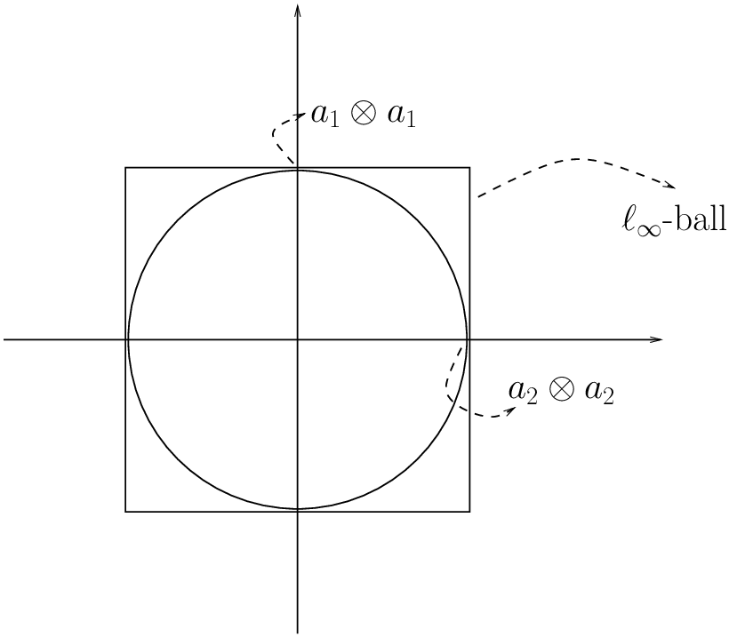
    Refer to caption
    Figure 1: If ai⊗aia_{i}\otimes a_{i} were orthonormal then they would also be the extremal points of the matrix operator norm in the Frobenius ball of 𝒜\mathcal{A}.

    We therefore consider the following robust nonconvex program

    arg​max​‖M‖,s.t.M∈𝒜~,‖M‖F≤1,{\rm arg\ max}\ \|M\|,\quad{\rm s.t.}\quad M\in\widetilde{\mathcal{A}},\|M\|_{F}\leq 1,

    searching for extremal matrices of the operator norm within the Frobenius ball, and we prove with Theorem 6.5 that its (local) maximizing solutions have first singular vectors a^i\hat{a}_{i} which are approximations to any one aia_{i} up to sign. Conversely, we also show in Proposition 6.7 that every ai⊗aia_{i}\otimes a_{i} can be approximated by a local maximizer. The solution of this minimization problem is approached by an iterative gradient ascent-type algorithm, Algorithm 6.2, with Theorem 6.10 establishing its local convergence.

  • 5.

    (Identification of activation functions or ridge profiles) Once the weights are recovered (up to sign) it is not hard to build approximating ridge profiles g^i\hat{g}_{i} and construct an approximation f^\hat{f} of the full network. The construction is summarized as follows: Let (b^j)j=1m(\hat{b}_{j})_{j=1}^{m} be the dual basis to (a^j)j=1m(\hat{a}_{j})_{j=1}^{m}, then one can define g^j​(t):=f⁡(t​b^j)\hat{g}_{j}(t):=f(t\hat{b}_{j}), t∈(−1/∥b^j∥2,1/∥b^j∥2)t\in(-1/\|\hat{b}_{j}\|_{2},1/\|\hat{b}_{j}\|_{2}) and f^​(x):=∑j=1mg^j​(⟨a^j,x⟩)\displaystyle\hat{f}(x):=\sum_{j=1}^{m}\hat{g}_{j}(\langle\hat{a}_{j},x\rangle). We show in the concluding Theorem 7.2 that f^\hat{f} is a good uniform approximation to the original network.

Remark 1.

(Whitening) As we have seen in the step 4, the problem of the identification of near rank-11 matrices in 𝒜~≈𝒜=span⁡{ai⊗ai,i=1,…,m}⊂ℝm×m\widetilde{\mathcal{A}}\approx{\mathcal{A}}=\operatorname{span}\{a_{i}\otimes a_{i},i=1,\dots,m\}\subset\mathbb{R}^{m\times m} is greatly simplified if one can assume that {a1,…,am}\{a_{1},\dots,a_{m}\} are nearly orthonormal vectors. If this condition is not fulfilled, we propose an additional step called whitening, which may be evoked between the steps 3 and 4 above. Indeed, we prove in Section 8 that, without loss of generality, we can always assume that the weights are nearly orthonormal. For this sake, we consider any positive definite matrix G~∈𝒜~\widetilde{G}\in\widetilde{\mathcal{A}} of ‖G~‖F=1\|\widetilde{G}\|_{F}=1 with maximal smallest eigenvalue and compute its singular value or spectral decomposition G~=U~​D~​U~T.\widetilde{G}=\widetilde{U}\widetilde{D}\widetilde{U}^{T}. If we now denote W~=D~−12​U~T\widetilde{W}=\widetilde{D}^{-\frac{1}{2}}\widetilde{U}^{T} the so-called whitening matrix, then we show in Theorem 8.3 that the system of vectors {W~ai:i=1,…,m}\{\widetilde{W}a_{i}:i=1,\dots,m\} defines a near-orthogonal basis. In view of the simple reformulation

f⁡(W~T​x)=∑i=1mgi​(⟨ai,W~T​x⟩)=∑i=1mg~i​(⟨W~​ai/‖W~​ai‖2,x⟩)=f~​(x),f(\widetilde{W}^{T}x)=\sum_{i=1}^{m}g_{i}(\langle a_{i},\widetilde{W}^{T}x\rangle)=\sum_{i=1}^{m}\tilde{g}_{i}(\langle\widetilde{W}a_{i}/\|\widetilde{W}a_{i}\|_{2},x\rangle)=\tilde{f}(x),

for g~i​(t)=gi​(‖W~​ai‖2​t)\tilde{g}_{i}(t)=g_{i}(\|\widetilde{W}a_{i}\|_{2}t), we can further assume without loss of generality that the vectors {ai:i=1,…,m}\{a_{i}:i=1,\dots,m\} are nearly orthonormal in first place.

1.4 Main result of the paper

At this point, it is worth to summarize all the construction through the different algorithms and intermediate results outlined above in a single higher level result, which we specify for the case of active sampling, exclusively for the sake of simplicity. A similar statement would hold also for the case of passive sampling, which allows for more generic distributions.

We introduce two matrices. First we shall assume that the matrix

J[f]:=∫𝕊d−1∇f(x)∇f(x)Tdμ𝕊d−1(x)J[f]:=\int_{{\mathbb{S}}^{d-1}}\nabla f(x)\nabla f(x)^{T}d\mu_{{\mathbb{S}}^{d-1}}(x) (1.5)

has maximal rank mm, being μ𝕊d−1\mu_{{\mathbb{S}}^{d-1}}22 2 The use of the uniform measure on the sphere for active sampling is by no means a restriction, more general distributions could be used with no significant difference in the results. the uniform measure on the sphere 𝕊d−1{\mathbb{S}}^{d-1}. The matrix J⁡[f]J[f] ensures that sampling approximate gradients of the network ff uniformly on the sphere is gathering enough information for the active subspace A=span⁡{a1,…,am}A=\operatorname{span}\{a_{1},\dots,a_{m}\} to be fully, robustly, and constructively identifiable by simple PCA. Then we consider also the matrix

H2​[f]:=∫𝕊m−1vec⁡(∇2f​(x))⊗vec⁡(∇2f​(x))​d​μ𝕊m−1​(x)H_{2}[f]:=\int_{\mathbb{S}^{m-1}}\operatorname{vec}(\nabla^{2}f(x))\otimes\operatorname{vec}(\nabla^{2}f(x))d\mu_{\mathbb{S}^{m-1}}(x)

of rank mm (the symbol vec⁡(∇2f​(x))\operatorname{vec}(\nabla^{2}f(x)) stands for the vectorization of the Hessian of ff, see (4.2) for its precise definition). The matrix H2​[f]H_{2}[f] also ensures that sampling approximate Hessians of the network ff uniformly on the sphere is gathering enough information for the active subspace 𝒜=span⁡{a1⊗a1,…,am⊗am}\mathcal{A}=\operatorname{span}\{a_{1}\otimes a_{1},\dots,a_{m}\otimes a_{m}\} to be fully, robustly, and constructively identifiable by simple PCA.

Theorem 1.1.

Let m≤dm\leq d and let ff be a real-valued function defined on the neighborhood of B1dB_{1}^{d}, which takes the form

f⁡(x)=∑i=1mgi​(⟨ai,x⟩),f(x)=\sum_{i=1}^{m}g_{i}(\langle a_{i},x\rangle),

where gi,i=1,…,m,g_{i},i=1,\dots,m, are three times continuously differentiable on a neighborhood of [−1,1][-1,1] and {a1,…,am}⊂ℝd\{a_{1},\dots,a_{m}\}\subset\mathbb{R}^{d} are linearly independent. We additionally assume both J⁡[f]J[f] and H2​[f]H_{2}[f] of maximal rank mm and well-conditioned. Let ϵ>0\epsilon>0. Then Algorithms 2.1-6.1 use at most m𝒳​[(d+1)+(m+1)​(m+2)/2]m_{\mathcal{X}}[(d+1)+(m+1)(m+2)/2] random exact point evaluations of ff, which correspond to numerical differentiation of ff with step-size ϵ\epsilon, and they construct approximations {a^1,…,a^m}\{\hat{a}_{1},\dots,\hat{a}_{m}\} of the ridge directions {a1,…,am}\{a_{1},\dots,a_{m}\} up to a sign change for which

(∑i=1m‖a^i−ai‖22)1/2≲ϵ,\bigg(\sum_{i=1}^{m}\|\hat{a}_{i}-a_{i}\|_{2}^{2}\bigg)^{1/2}\lesssim\epsilon, (1.6)

with probability at least 1−m​exp⁡(−m𝒳​C2​m2)1-m\exp\Bigl(-\frac{m_{\mathcal{X}}C}{2m^{2}}\Bigr) for suitable C>0C>0. Moreover, Algorithm 7.1 constructs an approximating function f^:B1d→ℝ\hat{f}:B_{1}^{d}\to\mathbb{R} of the form

f^​(x)=∑i=1mg^i​(⟨a^i,x⟩),\hat{f}(x)=\sum_{i=1}^{m}\hat{g}_{i}(\langle\hat{a}_{i},x\rangle),

such that

‖f−f^‖L∞​(B1d)≲ϵ.\|f-\hat{f}\|_{L_{\infty}(B^{d}_{1})}\lesssim\epsilon. (1.7)

The constant C>0C>0 as well as the asymptotic constants in (1.6) and (1.7) may depend on the smoothness properties of gig_{i} and the mt​hm^{th} singular value of J⁡[f]J[f] and H2​[f]H_{2}[f]. Furthermore, the constants in (1.6) and (1.7) may depend also polynomially on mm.

Let us remark, that Algorithms 2.1-6.1 realize the statement of Theorem 1.1 only when the vectors a1,…,ama_{1},\dots,a_{m} are close to an orthonormal basis in the sense of Definition 5.1. If this is not the case, it might be necessary to perform also the whitening step of Section 8.

In absence of noise on the point evaluations of ff as in Theorem 1.1, the usage of more point evaluations improves the accuracy in (1.6) and (1.7) only up to a limit posed by the numerical differentiation, but it increases the probability of success arbitrarily close to one. The result would need to be significantly modified in case of noise on the active point evaluations of ff in order to deal with stability issues determined by employing finite differences in order to approximate the gradient and the Hessian of ff. Contrary to most results available in the literature [3, 33, 45, 62], our final estimate (1.7) holds in the uniform norm, which is deterministic once the weights are correctly identified. In fact, probabilistic least squares error estimates usually investigated in the literature may appear to successfully circumvent the curse of dimensionality, but they are obtained at the practically relevant price of not ensuring uniform error bounds. Not only we avoid the curse of dimensionality, but we also do not compromise on the uniform bound.

In the setting of passive sampling, we assume that the values f⁡(x1),…,f⁡(xm𝒳)f(x_{1}),\dots,f(x_{m_{\mathcal{X}}}) were sampled in points x1,…,xm𝒳x_{1},\dots,x_{m_{\mathcal{X}}}, which are chosen independently with respect to a probability distribution μ\mu on B1d.B_{1}^{d}. Here, we assume that its density p⁡(x)p(x) is smooth and known in advance. Using Stein’s lemma [59] or integration by parts in a way similar to [33] and [40], we transfer our analysis also to the setting of passive sampling, leading first to the reduction of dimension from dd to m≤dm\leq d and then to the approximation of 𝒜=span{a1⊗a1,…,am⊗am}{\mathcal{A}}=\operatornamewithlimits{span}\{a_{1}\otimes a_{1},\dots,a_{m}\otimes a_{m}\}. Due to the non-local nature of the sampling process, it is rather easy to incorporate noise. Similarly to the active sampling, our main tools are the matrix concentration inequalities [1, 51, 55, 65].

We conclude this introduction by mentioning that this paper, besides the specific application on identification of shallow neural networks, contains results of independent mathematical and computational interest. First of all, we proved that stable whitening of matrices is constructively attainable, see Section 8. This seems to disprove a common belief in the literature, see, e.g., [33], that the use of third or higher order tensors can not be avoided. Moreover, we introduced a new nonconvex optimization (6.1) with no spurious local minimizers, which allows identifying robustly 11-rank matrices in linear subspaces of symmetric matrices, see Section 6 and Section 6.2. We provide a simple and efficient iterative algorithm to perform such an optimization, Section 6.3. Similar problems appeared recently in the literature and are of independent interest [49, 54].

2 Active subspace identification

As previously mentioned in the introduction, as soon as we can produce a subspace A~⊂ℝd\tilde{A}\subset\mathbb{R}^{d} approximating A=span⁡{a1,…,am}A=\operatorname{span}\{a_{1},\dots,a_{m}\}, we can eventually reduce the problem of approximating a sum of ridge functions in ℝd\mathbb{R}^{d} to the same problem in ℝm\mathbb{R}^{m}, preserving even the near-orthonormality, cf. Remark 5. In this section we describe two different methods of identification of AA. The first one applies to the setting of active sampling. It is motivated by the results in [22] and makes use of first order differences. The second method is inspired by [33], and implements passive sampling under the assumption that we dispose of the probability density p⁡(x)p(x) of the point distribution of the samples.

2.1 Active sampling

We observe that the vector

∇f​(x)=∑i=1mgi′​(⟨ai,x⟩)​ai\nabla f(x)=\sum_{i=1}^{m}g_{i}^{\prime}(\langle a_{i},x\rangle)a_{i} (2.1)

lies in AA for every x∈ℝdx\in\mathbb{R}^{d}. We consider (2.1) for different x1,…,xm𝒳∈ℝdx_{1},\dots,x_{m_{\mathcal{X}}}\in\mathbb{R}^{d}, where m𝒳≥mm_{\mathcal{X}}\geq m. In a generic situation for the points xix_{i}’s, AA is likely given as the span of {∇f​(x1),…,∇f​(xm𝒳)}\{\nabla f(x_{1}),\dots,\nabla f(x_{m_{\mathcal{X}}})\}.

As we would like to use only function values of ff in our algorithms, we use for every j=1,…,dj=1,\dots,d and every k=1,…,m𝒳k=1,\dots,m_{\mathcal{X}} the Taylor’s expansion

∂∂ej​f​(xk)=f⁡(xk+ϵ​ej)−f⁡(xk)ϵ−[∂∂ej​f​(xk+ηj,k​ej)−∂∂ej​f​(xk)]\frac{\partial}{\partial e_{j}}f(x_{k})=\frac{f(x_{k}+\epsilon e_{j})-f(x_{k})}{\epsilon}-\Bigl[\frac{\partial}{\partial e_{j}}f(x_{k}+\eta_{j,k}e_{j})-\frac{\partial}{\partial e_{j}}f(x_{k})\Bigr] (2.2)

for some ηj,k∈[0,ϵ]\eta_{j,k}\in[0,\epsilon]. We recast the d×m𝒳d\times m_{\mathcal{X}} instances of (2.2) into the matrix notation

X=Y−ℰ,X=Y-{\mathcal{E}}, (2.3)

where

Xj,k\displaystyle X_{j,k} =∂∂ej​f​(xk),Yj,k=f⁡(xk+ϵ​ej)−f⁡(xk)ϵ,\displaystyle=\frac{\partial}{\partial e_{j}}f(x_{k}),\qquad Y_{j,k}=\frac{f(x_{k}+\epsilon e_{j})-f(x_{k})}{\epsilon}, (2.4)
and
ℰj,k\displaystyle{\mathcal{E}}_{j,k} =∂∂ej​f​(xk+ηj,k​ej)−∂∂ej​f​(xk)\displaystyle=\frac{\partial}{\partial e_{j}}f(x_{k}+\eta_{j,k}e_{j})-\frac{\partial}{\partial e_{j}}f(x_{k})

for j=1,…,dj=1,\dots,d and k=1,…,m𝒳k=1,\dots,m_{\mathcal{X}}. It follows from (2.1), that AA is the linear span of columns of XX. Naturally, we define A~\tilde{A} using the linear span of the singular vectors of YY corresponding to its mm largest singular values. This is formalized in the following algorithm.

Algorithm 2.1.
• Construct YY according to (2.4). • Compute the singular value decomposition of YT=(U~1U~2)​(Σ~100Σ~2)​(V~1TV~2T),Y^{T}=\left(\begin{array}[]{lll}\tilde{U}_{1}&\tilde{U}_{2}\end{array}\right)\left(\begin{array}[]{ll}\tilde{\Sigma}_{1}&0\\ 0&\tilde{\Sigma}_{2}\\ \end{array}\right)\left(\begin{array}[]{l}\tilde{V}_{1}^{T}\\ \tilde{V}_{2}^{T}\end{array}\right), where Σ~1\tilde{\Sigma}_{1} contains the mm largest singular values. • Set A~\tilde{A} to be the row space of V~1T\tilde{V}_{1}^{T}.

The aim of the rest of this section is to show, that A~\tilde{A} constructed in Algorithm 2.1 is in some sense close to AA. To be more specific, we need to bound ‖PA−PA~‖\|P_{A}-P_{\tilde{A}}\|, i.e. the operator or the Frobenius norm of the difference between the orthogonal projections onto AA and A~\tilde{A}, respectively. For this first approximation method we need the matrix J⁡[f]J[f], which was defined in (1.5) as

J[f]:=∫𝕊d−1∇f(x)∇f(x)Tdμ𝕊d−1(x).J[f]:=\int_{{\mathbb{S}}^{d-1}}\nabla f(x)\nabla f(x)^{T}d\mu_{{\mathbb{S}}^{d-1}}(x).

In some sense, it captures the contribution of each term in (1.2). As we want to recover all ridge profiles, we assume that J⁡[f]J[f] has the maximal rank mm and its non-zero singular values are bounded away from zero.

Lemma 2.1.

Assume the vectors (ai)i=1m(a_{i})_{i=1}^{m} linearly independent, and ‖ai‖2=1\|a_{i}\|_{2}=1 for all i=1,…,mi=1,\dots,m. Additionally assume

C1\displaystyle C_{1} :=maxi=1,…,m⁡max−1≤t≤1​|gi′​(t)|<∞.\displaystyle:=\max_{i=1,\dots,m}\,\max_{-1\leq t\leq 1}|g^{\prime}_{i}(t)|<\infty.

Suppose that σm​(J⁡[f])≥α>0\sigma_{m}(J[f])\geq\alpha>0, i.e., the mt​hm^{th} singular value of the matrix J⁡[f]J[f] is bounded away from zero. Then for any s∈(0,1)s\in(0,1) we have that

σm​(X)≥m𝒳​α​(1−s)\sigma_{m}(X)\geq\sqrt{m_{\mathcal{X}}\alpha(1-s)} (2.5)

with probability at least 1−m​exp⁡(−m𝒳​α​s22​C12​m2)1-m\exp\Bigl(-\frac{m_{\mathcal{X}}\alpha s^{2}}{2C_{1}^{2}m^{2}}\Bigr), where XX is constructed as in (2.3) for x1,…,xm𝒳∈𝕊d−1x_{1},\dots,x_{m_{\mathcal{X}}}\in{\mathbb{S}}^{d-1} drawn uniformly at random.

Proof.

The result will follow by a suitable application of Theorem 10.3 in the Appendix. We choose an orthonormal basis w1,…,wmw_{1},\dots,w_{m} of AA and denote by WW a d×md\times m matrix with columns w1,…,wm.w_{1},\dots,w_{m}. We observe that σj​(X)=σj​(WT​X)=σj​(WT​X​XT​W)\sigma_{j}(X)=\sigma_{j}(W^{T}X)=\sqrt{\sigma_{j}(W^{T}XX^{T}W)},

XXT=∑l=1m𝒳∇f(xl)∇f(xl)TXX^{T}=\sum_{l=1}^{m_{\mathcal{X}}}\nabla f(x_{l})\nabla f(x_{l})^{T}

and

WTXXTW=∑l=1m𝒳WT∇f(xl)∇f(xl)TW.W^{T}XX^{T}W=\sum_{l=1}^{m_{\mathcal{X}}}W^{T}\nabla f(x_{l})\nabla f(x_{l})^{T}W.

Furthermore, we obtain for every x∈ℝdx\in\mathbb{R}^{d}

σ1(WT∇f(x)∇f(x)TW)\displaystyle\sigma_{1}(W^{T}\nabla f(x)\nabla f(x)^{T}W) =σ1(∇f(x)∇f(x)T)=∥∇f(x)∇f(x)T∥F\displaystyle=\sigma_{1}(\nabla f(x)\nabla f(x)^{T})=\|\nabla f(x)\nabla f(x)^{T}\|_{F}
=‖∇f​(x)‖22=‖∑i=1mgi′​(⟨ai,x⟩)​ai‖22\displaystyle=\|\nabla f(x)\|_{2}^{2}{\color[rgb]{0,0,0}{=\left\|\sum_{i=1}^{m}g_{i}^{\prime}(\langle a_{i},x\rangle)a_{i}\right\|_{2}^{2}}} (2.6)
≤(∑i=1m|gi′​(⟨ai,x⟩)|⋅‖ai‖2)2≤C12​m2.\displaystyle{\color[rgb]{0,0,0}{\leq\left(\sum_{i=1}^{m}|g_{i}^{\prime}(\langle a_{i},x\rangle)|\cdot\|a_{i}\|_{2}\right)^{2}\leq C_{1}^{2}m^{2}.}}

Hence Xj=WT∇f(xj)∇f(xj)TWX_{j}=W^{T}\nabla f(x_{j})\nabla f(x_{j})^{T}W is a random m×mm\times m positive-semidefinite matrix, that is almost surely bounded. Moreover,

𝔼Xj=WT∫𝕊d−1∇f(x)∇f(x)Tdμ𝕊d−1(x)W=WTJ[f]W.{\mathbb{E}}\,X_{j}=W^{T}\int_{{\mathbb{S}}^{d-1}}\nabla f(x)\nabla f(x)^{T}d\mu_{{\mathbb{S}}^{d-1}}(x)W=W^{T}J[f]W.

We conclude that μmin=μmin​(∑j=1m𝒳𝔼​Xj)≥m𝒳​α\displaystyle\mu_{\min}=\mu_{\min}\Bigl(\sum_{j=1}^{m_{\mathcal{X}}}{\mathbb{E}}X_{j}\Bigr)\geq m_{\mathcal{X}}\alpha, and by Theorem 10.3 in the Appendix

σm​(X)=σm​(WT​X​XT​W)≥μmin​(1−s)≥m𝒳​α​(1−s)\sigma_{m}(X)=\sqrt{\sigma_{m}(W^{T}XX^{T}W)}\geq\sqrt{\mu_{\min}(1-s)}\geq\sqrt{m_{\mathcal{X}}\alpha(1-s)}

with probability at least

1−m​exp⁡(−μmin​s22​C12​m2)\displaystyle 1-m\exp\Bigl({-\frac{\mu_{\min}s^{2}}{2C_{1}^{2}m^{2}}}\Bigr) ≥1−m​exp⁡(−m𝒳​α​s22​C12​m2).∎\displaystyle\geq 1-m\exp\Bigl(-\frac{m_{\mathcal{X}}\alpha s^{2}}{2C_{1}^{2}m^{2}}\Bigr).\qed
Remark 2.

If we further assume that a1,…,ama_{1},\dots,a_{m} are ε\varepsilon-nearly-orthonormal and w1,…,wmw_{1},\dots,w_{m} are orthonormal vectors with

𝒮⁡(a1,…,am)=(∑i=1m‖ai−wi‖22)1/2≤ε,{\mathcal{S}}(a_{1},\dots,a_{m})=\biggl(\sum_{i=1}^{m}\|a_{i}-w_{i}\|_{2}^{2}\biggr)^{1/2}\leq\varepsilon,

we can improve (2.6) to

σ1(WT∇f(x)∇f(x)TW)\displaystyle\sigma_{1}(W^{T}\nabla f(x)\nabla f(x)^{T}W) ≤‖∇f​(x)‖22=‖∑i=1mgi′​(⟨ai,x⟩)​ai‖22\displaystyle\leq\|\nabla f(x)\|^{2}_{2}=\Bigl\|\sum_{i=1}^{m}g_{i}^{\prime}(\langle a_{i},x\rangle)a_{i}\Bigr\|^{2}_{2}
≤(‖∑i=1mgi′​(⟨ai,x⟩)​wi‖2+‖∑i=1mgi′​(⟨ai,x⟩)​(ai−wi)‖2)2\displaystyle\leq\biggl(\Bigl\|\sum_{i=1}^{m}g_{i}^{\prime}(\langle a_{i},x\rangle)w_{i}\Bigr\|_{2}+\Bigl\|\sum_{i=1}^{m}g_{i}^{\prime}(\langle a_{i},x\rangle)(a_{i}-w_{i})\Bigr\|_{2}\biggr)^{2}
≤[(∑i=1m|gi′​(⟨ai,x⟩)|2)1/2+∑i=1m|gi′​(⟨ai,x⟩)|⋅‖ai−wi‖2]2\displaystyle\leq\biggl[\Bigl(\sum_{i=1}^{m}|g_{i}^{\prime}(\langle a_{i},x\rangle)|^{2}\Bigr)^{1/2}+\sum_{i=1}^{m}|g_{i}^{\prime}(\langle a_{i},x\rangle)|\cdot\|a_{i}-w_{i}\|_{2}\biggr]^{2}
≤(1+ε)2​∑i=1m|gi′​(⟨ai,x⟩)|2≤C12​(1+ε)2​m.\displaystyle\leq(1+\varepsilon)^{2}\sum_{i=1}^{m}|g_{i}^{\prime}(\langle a_{i},x\rangle)|^{2}\leq C_{1}^{2}(1+\varepsilon)^{2}m.

The rest of the proof then follows in the same manner, only the probability changes to

1−m​exp⁡(−m𝒳​α​s22​C12​(1+ε)2​m).1-m\exp\Bigl(-\frac{m_{\mathcal{X}}\alpha s^{2}}{2C_{1}^{2}(1+\varepsilon)^{2}m}\Bigr).

The same remark applies also to Theorem 4.2 below.

The following theorem quantifies the distance between the subspace A~\tilde{A} constructed in Algorithm 2.1 and AA.

Theorem 2.2.

Assume the vectors (ai)i=1m(a_{i})_{i=1}^{m} linearly independent, and ‖ai‖2=1\|a_{i}\|_{2}=1 for all i=1,…,mi=1,\dots,m. Additionally assume that

C1\displaystyle C_{1} :=maxi=1,…,m⁡max−1≤t≤1​|gi′​(t)|<∞\displaystyle:=\max_{i=1,\dots,m}\,\max_{-1\leq t\leq 1}|g^{\prime}_{i}(t)|<\infty

and that the Lipschitz constants of all gj′,j=1,…,mg_{j}^{\prime},j=1,\dots,m, are bounded by C2<∞.C_{2}<\infty.

Let A~\tilde{A} be constructed as described in Algorithm 2.1 by sampling m𝒳​(d+1)m_{\mathcal{X}}(d+1) values of ff. Let 0<s<10<s<1, and assume σm​(J⁡[f])≥α>0.\sigma_{m}(J[f])\geq\alpha>0. Then

‖PA−PA~‖F≤2​C2​ϵ​mα⁡(1−s)−C2​ϵ​m\|P_{A}-P_{\tilde{A}}\|_{F}\leq\frac{2C_{2}\epsilon m}{\sqrt{\alpha(1-s)}-C_{2}\epsilon m}

with probability at least 1−m​exp⁡(−m𝒳​α​s22​m2​C12)1-m\exp\Bigl(-\frac{m_{\mathcal{X}}\alpha s^{2}}{2m^{2}C_{1}^{2}}\Bigr).

Proof.

We intend to apply the so-called Wedin’s bound, as recalled in Theorem 10.2 in the Appendix, to estimate the distance between AA and A~\tilde{A}. If we choose B=XTB=X^{T} and B~=YT\tilde{B}=Y^{T}, we get Σ2=0\Sigma_{2}=0 and we observe that (10.8) and (10.9) are satisfied with α¯=σm​(YT)\bar{\alpha}=\sigma_{m}(Y^{T}). Therefore, Theorem 10.2 implies

‖PA−PA~‖F\displaystyle\|P_{A}-P_{\tilde{A}}\|_{F} =‖V1​V1T−V~1​V~1T‖F≤2​‖X−Y‖Fσm​(YT)\displaystyle=\|V_{1}V^{T}_{1}-\tilde{V}_{1}\tilde{V}_{1}^{T}\|_{F}\leq\frac{2\|X-Y\|_{F}}{\sigma_{m}(Y^{T})}
≤2​‖X−Y‖Fσm​(XT)−‖X−Y‖F,\displaystyle\leq\frac{2\|X-Y\|_{F}}{\sigma_{m}(X^{T})-\|X-Y\|_{F}}, (2.7)

where we have used Weyl’s inequality |σm​(XT)−σm​(YT)|≤‖X−Y‖F|\sigma_{m}(X^{T})-\sigma_{m}(Y^{T})|\leq\|X-Y\|_{F} in the last step. To continue in (2.7), we have to estimate ‖X−Y‖F\|X-Y\|_{F} and σm​(XT)\sigma_{m}(X^{T}).

We use the relation

|∂∂ej​f​(xk+ηj,k​ej)−∂∂ej​f​(xk)|=|∑i=1m[gi′​(⟨ai,xk+ηj,k​ej⟩)−gi′​(⟨ai,xk⟩)]​ai,j|≤C2​ϵ​∑i=1mai,j2\Bigl|\frac{\partial}{\partial e_{j}}f(x_{k}+\eta_{j,k}e_{j})-\frac{\partial}{\partial e_{j}}f(x_{k})\Bigr|=\Bigl|\sum_{i=1}^{m}[g^{\prime}_{i}(\langle a_{i},x_{k}+\eta_{j,k}e_{j}\rangle)-g^{\prime}_{i}(\langle a_{i},x_{k}\rangle)]a_{i,j}\Bigr|\leq C_{2}\epsilon\sum_{i=1}^{m}a_{i,j}^{2}

to obtain the estimate

‖X−Y‖F\displaystyle\|X-Y\|_{F} =‖ℰ‖F≤C2​ϵ​(∑k=1m𝒳∑j=1d(∑i=1mai,j2)2)1/2\displaystyle=\|{\mathcal{E}}\|_{F}\leq C_{2}\epsilon\Bigl(\sum_{k=1}^{m_{\mathcal{X}}}\sum_{j=1}^{d}\Bigl(\sum_{i=1}^{m}a_{i,j}^{2}\Bigr)^{2}\Bigr)^{1/2} (2.8)
≤C2​ϵ​m𝒳​∑j=1d∑i=1mai,j2=C2​ϵ​m𝒳​m.\displaystyle\leq C_{2}\epsilon\sqrt{m_{\mathcal{X}}}\sum_{j=1}^{d}\sum_{i=1}^{m}a_{i,j}^{2}=C_{2}\epsilon\sqrt{m_{\mathcal{X}}}m.

The statement now follows by a combination of (2.7) with (2.8) and (2.5). ∎

Remark 3.

The same argument as in the proof of Theorem 2.2 allows to show that

σm​(Y)−σm+1​(Y)≥m𝒳​(α⁡(1−s)−2​C2​ϵ​m)\sigma_{m}(Y)-\sigma_{m+1}(Y)\geq\sqrt{m_{\mathcal{X}}}(\sqrt{\alpha(1-s)}-2C_{2}\epsilon m)

with the same probability as before. Hence, for ϵ\epsilon small enough and m𝒳m_{\mathcal{X}} large, there is (with high probability) a gap in the spectrum of YY between σm​(Y)\sigma_{m}(Y) and σm+1​(Y)\sigma_{m+1}(Y). This can be used to detect mm if it is unknown.

2.2 Passive sampling

In the previous sections we investigated the identification of the subspace AA when the sample points of f⁡(x)f(x) can be actively chosen. For that we used classical differentiation and Taylor’s residuals and we assumed exact evaluations of the function. In this section, we discuss the approximation of AA in the more realistic scenario where the distribution of the sampling points is known, but not actively chosen, and the point evaluations are affected by noise.

As in [33], we assume that we are given a probability distribution μ\mu, whose density p⁡(x)p(x) is known or has been previously estimated from empirical data [18]. For simplicity we assume supp⁡(p)⊂B1d\operatorname{supp}(p)\subset B_{1}^{d}. We also assume that we are given a probability space (𝒱,π)(\mathcal{V},\pi) and a suitable collection of 𝒞c1\mathcal{C}_{c}^{1} functions φν:ℝd→ℝ\varphi_{\nu}:\mathbb{R}^{d}\to\mathbb{R}, for ν∈𝒱\nu\in\mathcal{V}, with the properties

supp⁡φν⊂B1d​ for all ​ν∈𝒱,maxν∈𝒱⁡maxx∈B1d​‖∇φν​(x)p⁡(x)‖2≤C𝒱,\operatorname{supp}\varphi_{\nu}\subset B_{1}^{d}\mbox{ for all }\nu\in\mathcal{V},\quad\max_{\nu\in\mathcal{V}}\max_{x\in B_{1}^{d}}\left\|\frac{\nabla\varphi_{\nu}(x)}{p(x)}\right\|_{2}\leq C_{\mathcal{V}}, (2.9)

and for which the matrix

J𝒱​[f]=∫𝒱(∫ℝd∇f​(x)​φν​(x)​𝑑x)​(∫ℝd∇f​(x)​φν​(x)​𝑑x)T​𝑑π​(ν)J_{\mathcal{V}}[f]=\int_{\mathcal{V}}\left(\int_{\mathbb{R}^{d}}\nabla f(x)\varphi_{\nu}(x)dx\right)\left(\int_{\mathbb{R}^{d}}\nabla f(x)\varphi_{\nu}(x)dx\right)^{T}d\pi(\nu) (2.10)

has rank mm.

Remark 4.
  • (i)

    The probability space (𝒱,π)(\mathcal{V},\pi), the set of functions {φν:ν∈𝒱}\{\varphi_{\nu}:\nu\in\mathcal{V}\}, and the full-rank condition for J𝒱​[f]J_{\mathcal{V}}[f] may appear abstract and a bit implicit at the first look. We clarify their role first in the most simple setting when m=1m=1, g⁡(t)=tg(t)=t and 𝒱={0}.{\mathcal{V}}=\{0\}. Then f⁡(x)=g⁡(⟨a,x⟩)=⟨a,x⟩f(x)=g(\langle a,x\rangle)=\langle a,x\rangle and (2.10) becomes

    J𝒱​[f]=a​aT⋅(∫ℝdφ0​(x)​𝑑x)2.J_{\mathcal{V}}[f]=aa^{T}\cdot\left(\int_{\mathbb{R}^{d}}\varphi_{0}(x)dx\right)^{2}.

    It will turn out later (cf. Lemma 10.1 and Theorem 2.3), that we need to choose φ0:B1d→ℝ\varphi_{0}:B_{1}^{d}\to\mathbb{R}, such that α/C𝒱2\alpha/C_{\mathcal{V}}^{2} is as large as possible, where α=σ1​(J𝒱​[f])\alpha=\sigma_{1}(J_{\mathcal{V}}[f]) stands for the spectral norm of J𝒱​[f]J_{\mathcal{V}}[f]. Finally, if p⁡(x)=1ωdp(x)=\frac{1}{\omega_{d}} for every x∈B1dx\in B_{1}^{d} with ωd\omega_{d} denoting the Lebesgue volume of B1dB_{1}^{d} and φ0\varphi_{0} is radial with φ0​(1)=0\varphi_{0}(1)=0, we get

    αC𝒱2\displaystyle\frac{\alpha}{C_{\mathcal{V}}^{2}} =(∫ℝdφ0​(x)​𝑑x)2ωd2​maxx∈B1d​‖∇φ0​(x)‖22=(∫01d​ωd​rd−1​φ0​(r)​𝑑r)2ωd2​max0<r<1​|φ0′​(r)|2≤d2​(∫01∫r11​𝑑s​rd−1​𝑑r)2\displaystyle=\frac{\displaystyle\left(\int_{\mathbb{R}^{d}}\varphi_{0}(x)dx\right)^{2}}{\displaystyle\omega_{d}^{2}\max_{x\in B_{1}^{d}}\|\nabla\varphi_{0}(x)\|^{2}_{2}}=\frac{\displaystyle\left(\int_{0}^{1}d\omega_{d}r^{d-1}\varphi_{0}(r)dr\right)^{2}}{\displaystyle\omega_{d}^{2}\max_{0<r<1}|\varphi^{\prime}_{0}(r)|^{2}}\leq d^{2}\left(\int_{0}^{1}\int_{r}^{1}1dsr^{d-1}dr\right)^{2}
    =d2​(∫01(1−r)​rd−1​𝑑r)2=d2​(1d−1d+1)2=1(d+1)2.\displaystyle=d^{2}\left(\int_{0}^{1}(1-r)r^{d-1}dr\right)^{2}=d^{2}\left(\frac{1}{d}-\frac{1}{d+1}\right)^{2}=\frac{1}{(d+1)^{2}}.

    We observe that the conditions on {φν:ν∈𝒱}\{\varphi_{\nu}:\nu\in\mathcal{V}\} and J𝒱​[f]J_{\mathcal{V}}[f] may include an implicit dependence on dd. This is in accordance with the very well-known fact, that even the identification of one neuron (or one ridge function) can suffer the curse of dimension if we do not pose any additional restrictions on its activation function or its weights, cf. [4, 22, 44].

  • (ii)

    In fact, one may relate (𝒱,π)(\mathcal{V},\pi) and {φν:ν∈𝒱}\{\varphi_{\nu}:\nu\in\mathcal{V}\} directly to the density pp as follows. We first consider a bounded resolution of the identity, i.e., a set of nonnegative smooth and compactly supported functions ψν≥0\psi_{\nu}\geq 0 such that ∫𝒱ψν​(x)​𝑑π​(ν)≡1\int_{\mathcal{V}}\psi_{\nu}(x)d\pi(\nu)\equiv 1 for all x∈B1dx\in B_{1}^{d} and maxν∈𝒱⁡maxx∈B1d​{|ψν​(x)|,‖∇ψν​(x)‖2}≤CΨ\max_{\nu\in\mathcal{V}}\max_{x\in B_{1}^{d}}\{|\psi_{\nu}(x)|,\|\nabla\psi_{\nu}(x)\|_{2}\}\leq C_{\Psi}. In case the set 𝒱\mathcal{V} is discrete, then {ψν:ν∈𝒱}\{\psi_{\nu}:\nu\in\mathcal{V}\} is simply a classical bounded partition of the unity. Additionally we pick yet another bounded and smooth function q≥0q\geq 0 such that maxx∈B1d⁡{q⁡(x)p⁡(x),‖∇q​(x)p⁡(x)‖2}≤Cq\max_{x\in B_{1}^{d}}\{\frac{q(x)}{p(x)},\|\frac{\nabla q(x)}{p(x)}\|_{2}\}\leq C_{q}.

    Then, one can define

    φν​(x)=ψν​(x)​q​(x),\varphi_{\nu}(x)=\psi_{\nu}(x)q(x),

    and it is not difficult to show that conditions (2.9) are fulfilled. In fact, for densities pp with bounded derivatives, e.g., Gaussian mixtures, one could choose for instance q⁡(x)=12​p​(x)2q(x)=\frac{1}{2}p(x)^{2}. In fact, in this case, q⁡(x)/p⁡(x)=12​p​(x)q(x)/p(x)=\frac{1}{2}p(x) and ∇q​(x)/p⁡(x)=∇p​(x)\nabla q(x)/p(x)=\nabla p(x). Moreover, the matrix

    J𝒱​[f]=∫𝒱(∫ℝd∇f​(x)​ψν​(x)​q​(x)​𝑑x)​(∫ℝd∇f​(x)​ψν​(x)​q​(x)​𝑑x)T​𝑑π​(ν),J_{\mathcal{V}}[f]=\int_{\mathcal{V}}\left(\int_{\mathbb{R}^{d}}\nabla f(x)\psi_{\nu}(x)q(x)dx\right)\left(\int_{\mathbb{R}^{d}}\nabla f(x)\psi_{\nu}(x)q(x)dx\right)^{T}d\pi(\nu),

    would correspond to the superposition of “weighted local evaluations” of ∇f⊗∇f\nabla f\otimes\nabla f over the supports of the functions ψν\psi_{\nu} to build a full-rank matrix.

Now, differently from [33], we consider the following empirical vectors

Yj=−1N∑k=1N(f(xk)+nk)∇φνj​(xk)p⁡(xk)\displaystyle Y_{j}=-\frac{1}{N}\sum_{k=1}^{N}(f(x_{k})+n_{k})\frac{\nabla\varphi_{\nu_{j}}(x_{k})}{p(x_{k})} ≈\displaystyle\approx −∫ℝdf(x)∇φνj​(x)p⁡(x)p(x)dx\displaystyle-\int_{\mathbb{R}^{d}}f(x)\frac{\nabla\varphi_{\nu_{j}}(x)}{p(x)}p(x)dx (2.11)
=\displaystyle= ∫ℝd∇f​(x)​φνj​(x)​𝑑x\displaystyle\int_{\mathbb{R}^{d}}\nabla f(x)\varphi_{\nu_{j}}(x)dx
=\displaystyle= ∑i=1m(∫ℝdg′​(⟨ai,x⟩)​φνj​(x)​𝑑x)​ai,\displaystyle\sum_{i=1}^{m}\left(\int_{\mathbb{R}^{d}}g^{\prime}(\langle a_{i},x\rangle)\varphi_{\nu_{j}}(x)dx\right)a_{i},

generated at random by sampling i.i.d. νj∼π\nu_{j}\sim\pi, j=1,…,m𝒳j=1,\dots,m_{\mathcal{X}}. Here, the random variables nkn_{k} model the noise in the evaluation of the function ff in the point xkx_{k} and we will assume that nkn_{k} are independent bounded centered random variables, i.e.,

|nk|≤C𝒩​ with probability ​1, and ​𝔼​[nk]=0.|n_{k}|\leq C_{\mathcal{N}}\mbox{ with probability }1,\mbox{ and }\mathbb{E}[n_{k}]=0. (2.12)

The assumption that the noise is bounded can be relaxed to unbounded noise with thin tails (for instance sub-Gaussian noise) at the cost of adding in Theorem 2.3 below a negative term to the probability in the statement, which accounts for the probability that the noise realizations are in fact bounded. We define the matrix Y𝒱∈ℝd×m𝒳Y_{\mathcal{V}}\in\mathbb{R}^{d\times m_{\mathcal{X}}}, whose columns are YjY_{j}, for j=1,…,m𝒳j=1,\dots,m_{\mathcal{X}}. We similarly denote X𝒱∈ℝd×m𝒳X_{\mathcal{V}}\in\mathbb{R}^{d\times m_{\mathcal{X}}} the matrix with columns Xj=∫ℝd∇f​(x)​φνj​(x)​𝑑xX_{j}=\int_{\mathbb{R}^{d}}\nabla f(x)\varphi_{\nu_{j}}(x)dx. With similar arguments as Lemma 2.1 and Theorem 2.2 we can show the following result, whose proof is postponed to the Appendix.

Theorem 2.3.

Assume the vectors (ai)i=1m(a_{i})_{i=1}^{m} linearly independent, and ‖ai‖2=1\|a_{i}\|_{2}=1 for all i=1,…,mi=1,\dots,m. Additionally assume that

Cℓ\displaystyle C_{\ell} :=maxi=1,…,mmax−1≤t≤1|gi(ℓ)(t)|<∞,ℓ=0,1.\displaystyle:=\max_{i=1,\dots,m}\,\max_{-1\leq t\leq 1}|g^{(\ell)}_{i}(t)|<\infty,\quad\ell=0,1.

Let A~\tilde{A} be constructed as described in Algorithm 2.1 by substituting there YY with Y𝒱Y_{\mathcal{V}}, built by sampling NN values of ff as in (2.11). Let 0<s<10<s<1, and assume σm​(J𝒱​[f])≥α>0\sigma_{m}(J_{\mathcal{V}}[f])\geq\alpha>0. Then, for every 0<η<α⁡(1−s)0<\eta<\sqrt{\alpha(1-s)},

‖PA−PA~‖F≤2​ηα⁡(1−s)−η\|P_{A}-P_{\tilde{A}}\|_{F}\leq\frac{2\eta}{\sqrt{\alpha(1-s)}-\eta} (2.13)

with probability at least 1−exp⁡(−η2​N8​(2​m​Q)2+14)−m​exp⁡(−m𝒳​α​s22​(m​Q)2)1-{\exp\Bigl(-\frac{\eta^{2}N}{8(2mQ)^{2}}+\frac{1}{4}\Bigr)}-m\exp\Bigl(-\frac{m_{\mathcal{X}}\alpha s^{2}}{2(mQ)^{2}}\Bigr), where Q=(C0+C𝒩/m)​C𝒱Q=(C_{0}+C_{\mathcal{N}}/m)C_{\mathcal{V}}. As a consequence, for any ε>0\varepsilon>0 and δ>0\delta>0,

‖PA−PA~‖F≤ε\|P_{A}-P_{\tilde{A}}\|_{F}\leq\varepsilon (2.14)

with probability at least 1−δ1-\delta as soon as the number NN of sampling values of ff fulfills

N≥32​(2+ε)2​(m​Q)2​ln⁡(3/δ)ε2​α​(1−s).N\geq\frac{32(2+\varepsilon)^{2}(mQ)^{2}\ln(3/\delta)}{\varepsilon^{2}\alpha(1-s)}. (2.15)

3 Dimensionality reduction

The main aim of this section is Theorem 3.1, which allows to reduce the general case of identification of a shallow network where the input dimension is larger than the number of neurons, d≥md\geq m, to the case where d=md=m, hence, with a potentially significant dimensionality reduction. Due to the typical range of parameters we have in mind, this step is crucial in reducing the complexity of the approximation of (1.4).

Theorem 3.1 (Reduction to mm dimensions).

Let us consider a function

f⁡(x)=∑i=1mgi​(⟨ai,x⟩),x∈B1d,f(x)=\sum_{i=1}^{m}g_{i}(\langle a_{i},x\rangle),\quad x\in B_{1}^{d}, (3.1)

for m≤dm\leq d and we denote A=span⁡{a1,…,am}A=\operatorname{span}\{a_{1},\dots,a_{m}\}. Let us now fix a mm-dimensional subspace A~⊂ℝd\tilde{A}\subset\mathbb{R}^{d}, for which we choose an orthonormal basis {a~1,…,a~m}\{\tilde{a}_{1},\dots,\tilde{a}_{m}\}, so that A~=span⁡{a~1,…,a~m}\tilde{A}=\operatorname{span}\{\tilde{a}_{1},\dots,\tilde{a}_{m}\}.33 3 With a certain abuse of notation, we often use in this paper the symbol AA also to denote the matrix whose columns are the vectors {a1,…,am}\{a_{1},\dots,a_{m}\}. Similarly, we arrange the vectors a~i\tilde{a}_{i}’s as columns of matrix A~\tilde{A}. We denote by PAP_{A} and PA~=A~​A~TP_{\tilde{A}}=\tilde{A}{\tilde{A}}^{T} the orthogonal projections onto AA and A~\tilde{A}, respectively. Then the function

f~​(y)=∑i=1mgi​(⟨αi,y⟩),y∈B1m⊂ℝm,\tilde{f}(y)=\sum_{i=1}^{m}g_{i}(\langle\alpha_{i},y\rangle),\quad y\in B_{1}^{m}\subset\mathbb{R}^{m}, (3.2)

with αi=A~T​ai\alpha_{i}={\tilde{A}}^{T}a_{i} satisfies for any other function f^:ℝm→ℝ\hat{f}:\mathbb{R}^{m}\to\mathbb{R} the following estimate

∥f−f^(A~T⋅)∥∞≤∥f∥Lip∥PA−PA~∥+∥f~−f^∥∞.\|f-\hat{f}({\tilde{A}}^{T}\cdot)\|_{\infty}\leq\|f\|_{\operatorname{Lip}}\|P_{A}-P_{\tilde{A}}\|+\|\tilde{f}-\hat{f}\|_{\infty}. (3.3)

Moreover, for any other set of vectors {α^1,…,α^m}⊂ℝm\{\hat{\alpha}_{1},\dots,\hat{\alpha}_{m}\}\subset\mathbb{R}^{m},

‖ai−A~​α^i‖2≤‖PA−PA~‖+‖αi−α^i‖2.\|a_{i}-\tilde{A}\hat{\alpha}_{i}\|_{2}\leq\|P_{A}-P_{\tilde{A}}\|+\|\alpha_{i}-\hat{\alpha}_{i}\|_{2}. (3.4)
Proof.

Let x∈B1dx\in B_{1}^{d}. We have

|f⁡(x)−f^​(A~T​x)|\displaystyle|f(x)-\hat{f}({\tilde{A}}^{T}x)| ≤|f⁡(x)−f~​(A~T​x)|+|f~​(A~T​x)−f^​(A~T​x)|\displaystyle\leq|f(x)-\tilde{f}({\tilde{A}}^{T}x)|+|\tilde{f}({\tilde{A}}^{T}x)-\hat{f}({\tilde{A}}^{T}x)|
≤|f⁡(x)−f⁡(A~​A~T​x)|+‖f~−f^‖∞=|f⁡(PA​x)−f⁡(PA~​x)|+‖f~−f^‖∞\displaystyle\leq|f(x)-f({\tilde{A}}{\tilde{A}}^{T}x)|+\|\tilde{f}-\hat{f}\|_{\infty}=|f(P_{A}x)-f(P_{\tilde{A}}x)|+\|\tilde{f}-\hat{f}\|_{\infty}
≤‖f‖Lip⋅‖PA​x−PA~​x‖2+‖f~−f^‖∞.\displaystyle\leq\|f\|_{\rm Lip}\cdot\|P_{A}x-P_{\tilde{A}}x\|_{2}+\|\tilde{f}-\hat{f}\|_{\infty}.

If we take the supremum over x∈B1dx\in B_{1}^{d}, we get (3.3).

The proof of (3.4) follows from

‖ai−A~​α^i‖2\displaystyle\|a_{i}-\tilde{A}\hat{\alpha}_{i}\|_{2} ≤‖ai−A~​αi‖2+‖A~​(αi−α^i)‖2=‖(PA−PA~)​ai‖2+‖A~​(αi−α^i)‖2\displaystyle\leq\|a_{i}-\tilde{A}\alpha_{i}\|_{2}+\|\tilde{A}(\alpha_{i}-\hat{\alpha}_{i})\|_{2}=\|(P_{A}-P_{\tilde{A}})a_{i}\|_{2}+\|\tilde{A}(\alpha_{i}-\hat{\alpha}_{i})\|_{2}
≤‖PA−PA~‖+‖αi−α^i‖2.∎\displaystyle\leq\|P_{A}-P_{\tilde{A}}\|+\|\alpha_{i}-\hat{\alpha}_{i}\|_{2}.\qed

In view of Theorem 3.1, we start the identification of a sum of mm ridge functions (3.1) on ℝd\mathbb{R}^{d} by first approximating the subspace A=span⁡{a1,…,am}A=\operatorname{span}\{a_{1},\dots,a_{m}\} by another subspace A~{\tilde{A}}, such that the operator norm ‖PA−PA~‖\|P_{A}-P_{\tilde{A}}\| is small. Then we consider the function f~​(y)=f​(A~​y)\tilde{f}(y)=f(\tilde{A}y), which is a sum of mm ridge functions on ℝm\mathbb{R}^{m} with ridge profiles α1,…,αm\alpha_{1},\dots,\alpha_{m}. Naturally, we will not be able to recover them exactly and we will only obtain some good approximation {α^1,…,α^m}⊂ℝm\{\hat{\alpha}_{1},\dots,\hat{\alpha}_{m}\}\subset\mathbb{R}^{m}. Then (3.4) shows that the vectors A~​α^i{\tilde{A}}\hat{\alpha}_{i} approximate well the original ridge profiles aia_{i}. Finally, if f^\hat{f} is a uniform approximation of f~\tilde{f} on B1mB_{1}^{m}, then (3.3) implies that the function f^​(A~T​x)\hat{f}({\tilde{A}}^{T}x) is a uniform approximation of ff on B1dB_{1}^{d}.

Observe that the sampling of f~\tilde{f} can be easily transferred to sampling of ff by f~​(y)=f​(A~​y).\tilde{f}(y)=f({\tilde{A}}y).

4 Principal Hessian subspace

While first order differentiation provides information about the active subspace A=span⁡{a1,…,am}A=\operatorname{span}\left\{a_{1},\dots,a_{m}\right\}, we need to query higher order derivatives in order to access the individual weights a1,…,ama_{1},\dots,a_{m}. First of all we construct here an approximation 𝒜~\widetilde{\mathcal{A}} to the space 𝒜=span⁡{ai⊗ai,i=1,…,m}\mathcal{A}=\operatorname{span}\{a_{i}\otimes a_{i},i=1,\dots,m\}. As in the previous sections we describe two different methods of identification of 𝒜\mathcal{A}. The first one is by active sampling and makes use of second order differences. The second one implements passive sampling under the assumption that we dispose of the probability density p⁡(x)p(x) of the point distribution.

4.1 Active sampling

We start by generating again m𝒳∈ℕm_{\mathcal{X}}\in\mathbb{N} points xl∼μ𝕊m−1x_{l}\sim\mu_{\mathbb{S}^{m-1}}, l=1,…,m𝒳l=1,\dots,m_{\mathcal{X}} uniformly at random on the m−1m-1 dimensional sphere (remind that now we assume m=dm=d), and we define

(Δ⁡[f]​(xl))j,k=f⁡(xl+ϵ⁡(ej+ek))−f⁡(xl+ϵ​ej)−f⁡(xl+ϵ​ek)+f⁡(xl)ϵ2,j,k=1,…,m.(\Delta[f](x_{l}))_{j,k}=\frac{f(x_{l}+\epsilon(e_{j}+e_{k}))-f(x_{l}+\epsilon e_{j})-f(x_{l}+\epsilon e_{k})+f(x_{l})}{\epsilon^{2}},\quad j,k=1,\dots,m.

As Δ⁡[f]​(x)∼∇2f​(x)=∑i=1mgi′′​(⟨ai,x⟩)​ai⊗ai∈𝒜\Delta[f](x)\sim{\nabla^{2}f}(x)=\sum_{i=1}^{m}g_{i}^{\prime\prime}(\langle a_{i},x\rangle)a_{i}\otimes a_{i}\in\mathcal{A}, we define 𝒜~\widetilde{\mathcal{A}} as the mm-dimensional subspace approximating the points (Δ⁡[f]​(xl))l=1m𝒳(\Delta[f](x_{l}))_{l=1}^{m_{\mathcal{X}}} in the least-square sense. For later use we define YY the m2×m𝒳m^{2}\times m_{\mathcal{X}} matrix with columns vec⁡(Δ​[f]​(xl))\operatorname{vec}(\Delta[f](x_{l})), i.e.,

Y=(vec⁡(Δ⁡[f]​(x1))​|…|​vec⁡(Δ⁡[f]​(xm𝒳))CLOSE.Y=(\operatorname{vec}(\Delta[f](x_{1}))|\dots|\operatorname{vec}(\Delta[f](x_{m_{\mathcal{X}}})). (4.1)

We show below that 𝒜~\widetilde{\mathcal{A}} is indeed a good approximation to 𝒜\mathcal{A} by showing that the difference of the respective orthogonal projections ‖P𝒜−P𝒜~‖F→F\|P_{\mathcal{A}}-P_{\widetilde{\mathcal{A}}}\|_{F\to F} in the operator norm associated to the Frobenius norm of matrices is small with high probability, as soon as m𝒳m_{\mathcal{X}} is large enough.

We need now to introduce some notations to facilitate the presentation. We define the vectorization of a matrix A=(ai,j)i,j∈ℝm×mA=(a_{i,j})_{i,j}\in\mathbb{R}^{m\times m} as the column vector in ℝm2\mathbb{R}^{m^{2}}

vec(A)k:=a⌊k−1m⌋+1,(k−1modm)+1,k=1,…,m2.\operatorname{vec}(A)_{k}:=a_{\lfloor\frac{k-1}{m}\rfloor+1,(k-1\mod m)+1},\quad k=1,\dots,m^{2}. (4.2)

For two matrices A,B∈ℝm×mA,B\in\mathbb{R}^{m\times m} we define their vectorized tensor product by

A⊗vB:=vec⁡(A)⊗vec⁡(B)=vec⁡(A)​vec​(B)T.A\otimes_{v}B:=\operatorname{vec}(A)\otimes\operatorname{vec}(B)=\operatorname{vec}(A)\operatorname{vec}(B)^{T}. (4.3)

(Note that such a product of matrices does coincide neither with the Hadamard product nor with the Kronecker product.) Thanks to these definitions and notations we can introduce the matrix

H2​[f]:=∫𝕊m−1∇2f​(x)⊗v∇2f​(x)​d​μ𝕊m−1​(x).H_{2}[f]:=\int_{\mathbb{S}^{m-1}}{\nabla^{2}f}(x)\otimes_{v}{\nabla^{2}f}(x)d\mu_{\mathbb{S}^{m-1}}(x).

This m2×m2m^{2}\times m^{2} matrix plays exactly the same role as J⁡[f]J[f] in Section 2.1.

Algorithm 4.1.
• Construct YY as in (4.1). • Compute the singular value decomposition of YT=(U~1U~2)​(Σ~100Σ~2)​(V~1TV~2T),Y^{T}=\left(\begin{array}[]{lll}\widetilde{U}_{1}&\widetilde{U}_{2}\end{array}\right)\left(\begin{array}[]{ll}\widetilde{\Sigma}_{1}&0\\ 0&\widetilde{\Sigma}_{2}\\ \end{array}\right)\left(\begin{array}[]{l}\widetilde{V}_{1}^{T}\\ \widetilde{V}_{2}^{T}\end{array}\right), where Σ~1\widetilde{\Sigma}_{1} contains the mm largest singular values. • Set A~\widetilde{A} to be the space of matrices, whose vectorization lies in the row space of V~1T\widetilde{V}_{1}^{T}.

As we follow the same strategy as the one used in Section 2.1 to approximate the space A=span⁡{ai,i=1,…,m}A=\operatorname{span}\{a_{i},i=1,\dots,m\}, we limit ourselves to reformulate it in the context of the vector space of matrices 𝒜\mathcal{A}. We start with a technical estimate, which is essentially based on Taylor’s theorem.

Lemma 4.1.

Assume the vectors (ai)i=1m(a_{i})_{i=1}^{m} satisfy ‖ai‖2=1\|a_{i}\|_{2}=1 for all i=1,…,mi=1,\dots,m and assume that gj,j=1,…,mg_{j},j=1,\dots,m, are two times differentiable with the Lipschitz constant of all gj′′,j=1,…,mg_{j}^{\prime\prime},j=1,\dots,m bounded from above by C3>0.C_{3}>0. Then, for all x∈𝕊m−1x\in\mathbb{S}^{m-1},

‖∇2f​(x)−Δ⁡[f]​(x)‖F≤2​C3​m​ϵ.\|{\nabla^{2}f}(x)-\Delta[f](x)\|_{F}\leq 2C_{3}m\epsilon.
Proof.

Let g⁡(t)=f⁡(x+t​ej+ϵ​ek)−f⁡(x+t​ej)g(t)=f(x+te_{j}+\epsilon e_{k})-f(x+te_{j}), where 0≤t≤ϵ0\leq t\leq\epsilon. Then by the mean value theorem

(Δ​[f]​(x))j,k\displaystyle(\Delta[f](x))_{j,k} =g⁡(ϵ)−g⁡(0)ϵ2=g′​(ξ1)ϵ=∂f∂xj​(x+ξ1​ej+ϵ​ek)−∂f∂xj​(x+ξ1​ej)ϵ\displaystyle=\frac{g(\epsilon)-g(0)}{\epsilon^{2}}=\frac{g^{\prime}(\xi_{1})}{\epsilon}=\frac{\frac{\partial f}{\partial x_{j}}(x+\xi_{1}e_{j}+\epsilon e_{k})-\frac{\partial f}{\partial x_{j}}(x+\xi_{1}e_{j})}{\epsilon}
=∂2f∂xk​∂xj​(x+ξ1​ej+ξ2​ek),\displaystyle=\frac{\partial^{2}f}{\partial x_{k}\partial x_{j}}(x+\xi_{1}e_{j}+\xi_{2}e_{k}),

where 0<ξ1,ξ2<ϵ0<\xi_{1},\xi_{2}<\epsilon. Therefore

|(∇2f​(x))j,k−(Δ⁡[f]​(x))j,k|\displaystyle|(\nabla^{2}f(x))_{j,k}-(\Delta[f](x))_{j,k}| =|∂2f∂xk​∂xj​(x)−∂2f∂xk​∂xj​(x+ξ1​ej+ξ2​ek)|\displaystyle=\Bigl|\frac{\partial^{2}f}{\partial x_{k}\partial x_{j}}(x)-\frac{\partial^{2}f}{\partial x_{k}\partial x_{j}}(x+\xi_{1}e_{j}+\xi_{2}e_{k})\Bigr|
≤∑l=1m|gl′′​(⟨al,x⟩)−gl′′​(⟨al,x+ξ1​ej+ξ2​ek⟩)|⋅|al,j|⋅|al,k|\displaystyle\leq\sum_{l=1}^{m}\bigl|g_{l}^{\prime\prime}(\langle a_{l},x\rangle)-g^{\prime\prime}_{l}(\langle a_{l},x+\xi_{1}e_{j}+\xi_{2}e_{k}\rangle)\bigr|\cdot|a_{l,j}|\cdot|a_{l,k}|
≤C3​ϵ​∑l=1m|al,j|⋅|al,k|⋅(|al,j|+|al,k|).\displaystyle\leq C_{3}\epsilon\sum_{l=1}^{m}|a_{l,j}|\cdot|a_{l,k}|\cdot(|a_{l,j}|+|a_{l,k}|).

Using triangle inequality and ‖aj‖4≤‖aj‖2=1\|a_{j}\|_{4}\leq\|a_{j}\|_{2}=1, we estimate

‖∇2f​(x)−Δ⁡[f]​(x)‖F\displaystyle\|{\nabla^{2}f}(x)-\Delta[f](x)\|_{F} ≤2​C3​ϵ​[∑j,k=1m(∑i=1mai,j2​|ai,k|)2]1/2≤2​C3​ϵ​∑i=1m(∑j,k=1mai,j4​ai,k2)1/2\displaystyle\leq 2C_{3}\epsilon\left[\sum_{j,k=1}^{m}\Bigl(\sum_{i=1}^{m}a_{i,j}^{2}|a_{i,k}|\Bigr)^{2}\right]^{1/2}\leq 2C_{3}\epsilon\sum_{i=1}^{m}\Bigl(\sum_{j,k=1}^{m}a_{i,j}^{4}a_{i,k}^{2}\Bigr)^{1/2}
=2​C3​ϵ​∑i=1m[(∑j=1mai,j4)​(∑k=1mai,k2)]1/2≤2​C3​ϵ​m.\displaystyle=2C_{3}\epsilon\sum_{i=1}^{m}\biggl[\Bigl(\sum_{j=1}^{m}a_{i,j}^{4}\Bigr)\Bigl(\sum_{k=1}^{m}a_{i,k}^{2}\Bigr)\biggr]^{1/2}\leq 2C_{3}\epsilon m.

∎

Theorem 4.2.

Assume the vectors (ai)i=1m(a_{i})_{i=1}^{m} linearly independent, and ‖ai‖2=1\|a_{i}\|_{2}=1 for all i=1,…,mi=1,\dots,m. Additionally assume

Cj\displaystyle C_{j} :=maxi=1,…,mmax−1≤t≤1|gi(j)(t)|<∞,j=0,1,2.\displaystyle:=\max_{i=1,\dots,m}\max_{-1\leq t\leq 1}|g^{(j)}_{i}(t)|<\infty,\quad j=0,1,2.

Let 𝒜~\widetilde{\mathcal{A}} be constructed as described in Algorithm 4.1 by sampling m𝒳​[(m+1)​(m+2)/2]m_{\mathcal{X}}\left[(m+1)(m+2)/2\right] values of ff. Let 0<s<10<s<1, and assume σm​(H2​[f])≥α2>0\sigma_{m}(H_{2}[f])\geq\alpha_{2}>0, i.e., the mt​hm^{th} singular value of the matrix H2​[f]H_{2}[f] is bounded away from zero. Then

‖P𝒜−P𝒜~‖F→F≤4​C3​m​ϵα2​(1−s)−2​C3​m​ϵ\|P_{\mathcal{A}}-P_{\widetilde{\mathcal{A}}}\|_{F\to F}\leq\frac{4C_{3}m\epsilon}{\sqrt{\alpha_{2}(1-s)}-2C_{3}m\epsilon}

with probability at least 1−m​exp⁡(−m𝒳​α2​s22​m2​C22).1-m\exp\left(-\frac{m_{\mathcal{X}}\alpha_{2}s^{2}}{2m^{2}C_{2}^{2}}\right). In particular dim⁡(𝒜)=dim⁡(𝒜~)=m{\rm{dim}}(\mathcal{A})={\rm{dim}}(\widetilde{\mathcal{A}})=m.

Proof.

We define the matrices X,YX,Y whose columns are given by vec⁡(∇2f​(xj))\operatorname{vec}({\nabla^{2}f}(x_{j})), j=1,…,m𝒳j=1,\dots,m_{\mathcal{X}} and vec⁡(Δ​[f]​(xj))\operatorname{vec}(\Delta[f](x_{j})), j=1,…,m𝒳j=1,\dots,m_{\mathcal{X}} respectively, namely

X\displaystyle X =\displaystyle= (vec⁡(∇2f​(x1))​|…|​vec⁡(∇2f​(xm𝒳))),Y=(vec⁡(Δ⁡[f]​(x1))​|…|​vec⁡(Δ⁡[f]​(xm𝒳))).\displaystyle(\operatorname{vec}({\nabla^{2}f}(x_{1}))|\dots|\operatorname{vec}({\nabla^{2}f}(x_{m_{\mathcal{X}}}))),\quad Y=(\operatorname{vec}(\Delta[f](x_{1}))|\dots|\operatorname{vec}(\Delta[f](x_{m_{\mathcal{X}}}))).

Notice that these matrices have dimension m2×m𝒳m^{2}\times m_{\mathcal{X}}. As done in (2.7) and by assuming for the moment that σm​(X)≠0\sigma_{m}(X)\neq 0 (but obviously σm+1​(X)=0\sigma_{m+1}(X)=0 because the ∇2f​(xi){\nabla^{2}f}(x_{i})’s lie all in the mm-dimensional space 𝒜\mathcal{A}), we deduce the estimate

‖P𝒜−P𝒜~‖F→F≤2​‖X−Y‖Fσm​(X)−‖X−Y‖F,\|P_{\mathcal{A}}-P_{\widetilde{\mathcal{A}}}\|_{F\to F}\leq\frac{2\|X-Y\|_{F}}{\sigma_{m}(X)-\|X-Y\|_{F}}, (4.4)

as an application of Wedin’s bound, Theorem 10.2 in the Appendix. From Lemma 4.1 we easily deduce

‖X−Y‖F=(∑j=1m𝒳‖∇2f​(xj)−Δ⁡[f]​(xj)‖F2)1/2≤2​C3​ϵ​m​m𝒳.\|X-Y\|_{F}=\left(\sum_{j=1}^{m_{\mathcal{X}}}\|{\nabla^{2}f}(x_{j})-\Delta[f](x_{j})\|_{F}^{2}\right)^{1/2}\leq 2C_{3}\epsilon m\sqrt{m_{\mathcal{X}}}. (4.5)

In order to apply (4.4) we need finally to estimate σm​(X)\sigma_{m}(X) from below and we shall do it by using again the Chernoff’s bound for matrices Theorem 10.3.

Given an orthonormal basis {B1,…,Bm}\{B_{1},\dots,B_{m}\} for 𝒜\mathcal{A} we define the projector from ℝm2→ℝm\mathbb{R}^{m^{2}}\to\mathbb{R}^{m} given by P𝒜​v=(vec⁡(B1)T​v,…,vec⁡(Bm)T​v)P^{\mathcal{A}}v=(\operatorname{vec}(B_{1})^{T}v,\dots,\operatorname{vec}(B_{m})^{T}v) for any v∈ℝm2v\in\mathbb{R}^{m^{2}}. We additionally define with some abuse of notation

P𝒜​X:=(P𝒜​(vec⁡(∇2f​(x1)))​|…|​P𝒜​(vec⁡(∇2f​(xm𝒳)))).P^{\mathcal{A}}X:=(P^{\mathcal{A}}(\operatorname{vec}({\nabla^{2}f}(x_{1})))|\dots|P^{\mathcal{A}}(\operatorname{vec}({\nabla^{2}f}(x_{m_{\mathcal{X}}})))).

Notice that now this matrix has dimension m×m𝒳m\times m_{\mathcal{X}}. Thanks to the fact that P𝒜P^{\mathcal{A}} is an orthogonal transformation, we obtain the following equivalences

σm​(X)=σm​((P𝒜​X)​(P𝒜​X)T).\sigma_{m}(X)=\sqrt{\sigma_{m}((P^{\mathcal{A}}X)(P^{\mathcal{A}}X)^{T})}.

Hence to estimate σm​(X)\sigma_{m}(X), it is sufficient to do it for σm​((P𝒜​X)​(P𝒜​X)T)\sigma_{m}((P^{\mathcal{A}}X)(P^{\mathcal{A}}X)^{T}), whose argument is explicitly expressed as a sum

(P𝒜​X)​(P𝒜​X)T=∑j=1m𝒳Xj,(P^{\mathcal{A}}X)(P^{\mathcal{A}}X)^{T}=\sum_{j=1}^{m_{\mathcal{X}}}X_{j},

where

Xj=P𝒜​vec⁡(∇2f​(xj))⊗vec⁡(∇2f​(xj))​(P𝒜)T.X_{j}=P^{\mathcal{A}}\operatorname{vec}({\nabla^{2}f}(x_{j}))\otimes\operatorname{vec}({\nabla^{2}f}(x_{j}))(P^{\mathcal{A}})^{T}.

We wish to apply Theorem 10.3 for the sequence of positive semidefinite matrices X1,…,Xm𝒳X_{1},\dots,X_{m_{\mathcal{X}}}. We notice first that

𝔼​Xj=P𝒜​H2f​(P𝒜)T,\mathbb{E}X_{j}=P^{\mathcal{A}}H_{2}^{f}(P^{\mathcal{A}})^{T},

and therefore

μmin​(𝔼​Xj)≥m𝒳​α2.\mu_{\min}\left(\mathbb{E}X_{j}\right)\geq m_{\mathcal{X}}\alpha_{2}. (4.6)

Additionally, for every x∈𝕊m−1x\in\mathbb{S}^{m-1}

σ1​(P𝒜​vec⁡(∇2f​(x))⊗vec⁡(∇2f​(x))​(P𝒜)T)\displaystyle\sigma_{1}(P^{\mathcal{A}}\operatorname{vec}({\nabla^{2}f}(x))\otimes\operatorname{vec}({\nabla^{2}f}(x))(P^{\mathcal{A}})^{T}) =\displaystyle= σ1​(vec⁡(∇2f​(x))⊗vec⁡(∇2f​(x)))\displaystyle\sigma_{1}(\operatorname{vec}({\nabla^{2}f}(x))\otimes\operatorname{vec}({\nabla^{2}f}(x))) (4.7)
≤\displaystyle\leq ‖∇2f​(xj)‖F2\displaystyle\|{\nabla^{2}f}(x_{j})\|_{F}^{2}
=\displaystyle= ‖∑i=1mg′′​(⟨ai,x⟩)​ai⊗ai‖F2\displaystyle\Bigl\|\sum_{i=1}^{m}g^{\prime\prime}(\langle a_{i},x\rangle)a_{i}\otimes a_{i}\Bigr\|_{F}^{2}
≤\displaystyle\leq C22​m2.\displaystyle C_{2}^{2}m^{2}.

An application of Theorem 10.3 under conditions (4.6) and (4.7) yields

σm​(X)≥m𝒳​α2​(1−s),\sigma_{m}(X)\geq\sqrt{m_{\mathcal{X}}\alpha_{2}(1-s)}, (4.8)

with probability

1−m​exp⁡(−m𝒳​α2​s22​m2​C22).1-m\exp\left(-\frac{m_{\mathcal{X}}\alpha_{2}s^{2}}{2m^{2}C_{2}^{2}}\right).

We conclude from (4.5) and (4.8) that, with the same probability,

‖P𝒜−P𝒜~‖F→F≤4​C3​m​ϵα2​(1−s)−2​C3​m​ϵ.∎\|P_{\mathcal{A}}-P_{\widetilde{\mathcal{A}}}\|_{F\to F}\leq\frac{4C_{3}m\epsilon}{\sqrt{\alpha_{2}(1-s)}-2C_{3}m\epsilon}.\qed

4.2 Passive sampling

We again assume that we are given a probability space (𝒱,π)(\mathcal{V},\pi) and a suitable collection of 𝒞c2\mathcal{C}_{c}^{2} functions φν:ℝd→ℝ\varphi_{\nu}:\mathbb{R}^{d}\to\mathbb{R}, for ν∈𝒱\nu\in\mathcal{V}, with the properties

supp⁡φν⊂B1d​ for all ​ν∈𝒱,maxν∈𝒱⁡max⁡{∫ℝd|φν​(x)|​𝑑x,maxx∈B1d⁡‖∇2φν​(x)p⁡(x)‖F}≤C𝒱,2,\operatorname{supp}\varphi_{\nu}\subset B_{1}^{d}\mbox{ for all }\nu\in\mathcal{V},\quad\max_{\nu\in\mathcal{V}}\max\left\{\int_{\mathbb{R}^{d}}|\varphi_{\nu}(x)|dx,\max_{x\in B_{1}^{d}}\left\|\frac{\nabla^{2}\varphi_{\nu}(x)}{p(x)}\right\|_{F}\right\}\leq C_{\mathcal{V},2},

where in the latter bound we consider the Frobeniuns norm. Furthermore, we also assume that the matrix

H𝒱​[f]=∫𝒱(∫ℝd∇2f​(x)​φν​(x)​𝑑x)⊗v(∫ℝd∇2f​(x)​φν​(x)​𝑑x)T​𝑑π​(ν)H_{\mathcal{V}}[f]=\int_{\mathcal{V}}\left(\int_{\mathbb{R}^{d}}\nabla^{2}f(x)\varphi_{\nu}(x)dx\right)\otimes_{v}\left(\int_{\mathbb{R}^{d}}\nabla^{2}f(x)\varphi_{\nu}(x)dx\right)^{T}d\pi(\nu)

has full rank. We consider the following empirical vectors

Yj=vec⁡(1N​∑k=1N(f⁡(xk)+nk)​∇2φνj​(xk)p⁡(xk))\displaystyle Y_{j}=\operatorname{vec}\left(\frac{1}{N}\sum_{k=1}^{N}(f(x_{k})+n_{k})\frac{\nabla^{2}\varphi_{\nu_{j}}(x_{k})}{p(x_{k})}\right) ≈\displaystyle\approx vec⁡(∫ℝdf⁡(x)​∇2φνj​(x)p⁡(x)​p​(x)​𝑑x)\displaystyle\operatorname{vec}\left(\int_{\mathbb{R}^{d}}f(x)\frac{\nabla^{2}\varphi_{\nu_{j}}(x)}{p(x)}p(x)dx\right) (4.9)
=\displaystyle= vec⁡(∫ℝd∇2f​(x)​φνj​(x)​𝑑x)\displaystyle\operatorname{vec}\left(\int_{\mathbb{R}^{d}}\nabla^{2}f(x)\varphi_{\nu_{j}}(x)dx\right)
=\displaystyle= ∑i=1mvec⁡((∫ℝdg′′​(⟨ai,x⟩)​φνj​(x)​𝑑x)​ai⊗ai),\displaystyle\sum_{i=1}^{m}\operatorname{vec}\left(\left(\int_{\mathbb{R}^{d}}g^{\prime\prime}(\langle a_{i},x\rangle)\varphi_{\nu_{j}}(x)dx\right)a_{i}\otimes a_{i}\right),

generated at random by sampling i.i.d. νj∼π\nu_{j}\sim\pi, j=1,…,m𝒳j=1,\dots,m_{\mathcal{X}}, for nkn_{k} independent random bounded and centered noise fulfilling (2.12). We define the matrix Y𝒱,2∈ℝm2×m𝒳Y_{\mathcal{V},2}\in\mathbb{R}^{m^{2}\times m_{\mathcal{X}}}, whose columns are YjY_{j}, for j=1,…,m𝒳j=1,\dots,m_{\mathcal{X}}. We similarly denote X𝒱,2∈ℝm2×m𝒳X_{\mathcal{V},2}\in\mathbb{R}^{m^{2}\times m_{\mathcal{X}}} the matrix with columns Xj=vec⁡(∫ℝd∇2f​(x)​φνj​(x)​𝑑x)X_{j}=\operatorname{vec}\left(\int_{\mathbb{R}^{d}}\nabla^{2}f(x)\varphi_{\nu_{j}}(x)dx\right).

The proof of the following result resembles the proofs of Theorem 4.2 and Theorem 2.3 and is postponed to the Appendix.

Theorem 4.3.

Assume the vectors (ai)i=1m(a_{i})_{i=1}^{m} linearly independent, and ‖ai‖2=1\|a_{i}\|_{2}=1 for all i=1,…,mi=1,\dots,m. Additionally assume

Cj\displaystyle C_{j} :=maxi=1,…,mmax−1≤t≤1|gi(j)(t)|<∞,j=0,1,2.\displaystyle:=\max_{i=1,\dots,m}\max_{-1\leq t\leq 1}|g^{(j)}_{i}(t)|<\infty,\quad j=0,1,2.

Let 𝒜~\widetilde{\mathcal{A}} be constructed as described in Algorithm 4.1 by substituting there YY with Y𝒱,2Y_{\mathcal{V},2}, built by sampling NN values of ff as in (4.9). Let 0<s<10<s<1, and assume σm​(H𝒱​[f])≥α2>0\sigma_{m}(H_{\mathcal{V}}[f])\geq\alpha_{2}>0. Then, for 0<η<α2​(1−s)0<\eta<\sqrt{\alpha_{2}(1-s)},

‖P𝒜−P𝒜~‖F→F≤2​ηα2​(1−s)−η\|P_{\mathcal{A}}-P_{\widetilde{\mathcal{A}}}\|_{F\to F}\leq\frac{2\eta}{\sqrt{\alpha_{2}(1-s)}-\eta} (4.10)

with probability at least 1−exp⁡(−η2​N8​(2​m​Q)2+14)−m​exp⁡(−m𝒳​α2​s22​(m​Q)2)1-{\exp\left(-\frac{\eta^{2}N}{8(2mQ)^{2}}+\frac{1}{4}\right)}-m\exp\Bigl(-\frac{m_{\mathcal{X}}\alpha_{2}s^{2}}{2(mQ)^{2}}\Bigr), for Q=(max⁡{C0,C2}+C𝒩/m)​C𝒱,2Q=(\max\{C_{0},C_{2}\}+C_{\mathcal{N}}/m)C_{\mathcal{V},2}. As a consequence, for any ε>0\varepsilon>0 and δ>0\delta>0,

‖P𝒜−P𝒜~‖F→F≤ε,\|P_{\mathcal{A}}-P_{\widetilde{\mathcal{A}}}\|_{F\to F}\leq\varepsilon, (4.11)

with probability at least 1−δ1-\delta as soon as the number NN of sampling values of ff fulfills

N≥32​(2+ε)2​(m​Q)2​ln⁡(3/δ)ε2​α2​(1−s).N\geq\frac{32(2+\varepsilon)^{2}(mQ)^{2}\ln(3/\delta)}{\varepsilon^{2}\alpha_{2}(1-s)}. (4.12)

5 Near orthonormality

As we shall see in Section 6 and as pointed already in the Introduction, the problem of the identification of near rank-11 matrices in 𝒜~≈𝒜=span⁡{ai⊗ai,i=1,…,m}⊂ℝm×m\widetilde{\mathcal{A}}\approx{\mathcal{A}}=\operatorname{span}\{a_{i}\otimes a_{i},i=1,\dots,m\}\subset\mathbb{R}^{m\times m} is greatly simplified if one can assume that {a1,…,am}\{a_{1},\dots,a_{m}\} are nearly orthonormal vectors. In this section, we introduce the concept of near-orthonormality and its basic properties.

Definition 5.1.

We define

𝒮(α1,…,αm)=inf{(∑i=1m∥αi−wi∥22)1/2:w1,…,wmorthonormal basis inℝm}{\mathcal{S}}(\alpha_{1},\dots,\alpha_{m})=\inf\Bigl\{\Bigl(\sum_{i=1}^{m}\|\alpha_{i}-w_{i}\|_{2}^{2}\Bigr)^{1/2}:w_{1},\dots,w_{m}\quad\text{orthonormal basis in}\ \mathbb{R}^{m}\Bigr\} (5.1)

for every set {α1,…,αm}⊂ℝm\{\alpha_{1},\dots,\alpha_{m}\}\subset\mathbb{R}^{m}. We say that unit vectors a1,…,am∈ℝma_{1},\dots,a_{m}\in\mathbb{R}^{m} are ε\varepsilon-nearly-orthonormal, if 𝒮⁡(a1,…,am)≤ε{\mathcal{S}}(a_{1},\dots,a_{m})\leq\varepsilon for ε>0\varepsilon>0 relatively small.

Theorem 5.1.
  1. (i)

    Let a1,…,am∈ℝma_{1},\dots,a_{m}\in\mathbb{R}^{m} and let A∈ℝm×mA\in\mathbb{R}^{m\times m} be a matrix with columns a1,…,ama_{1},\dots,a_{m}. Then

    𝒮⁡(a1,…,am)=(∑i=1m(σi−1)2)1/2,{\mathcal{S}}(a_{1},\dots,a_{m})=\Bigl(\sum_{i=1}^{m}(\sigma_{i}-1)^{2}\Bigr)^{1/2},

    where σ1≥σ2≥⋯≥0\sigma_{1}\geq\sigma_{2}\geq\dots\geq 0 are the singular values of AA.

  2. (ii)

    Furthermore,

    𝒮⁡(a1,…,am)≤‖A​AT−Im‖F≤(‖A‖+1)​𝒮​(a1,…,am).{\mathcal{S}}(a_{1},\dots,a_{m})\leq\|AA^{T}-I_{m}\|_{F}\leq(\|A\|+1){\mathcal{S}}(a_{1},\dots,a_{m}).
Proof.
  1. (i)

    The result is very well known and the proof follows easily by singular value decomposition of A=U​Σ​VT.A=U\Sigma V^{T}. The closest orthogonal basis w1,…,wmw_{1},\dots,w_{m} is given as the columns of the matrix W=U​VT.W=UV^{T}.

  2. (ii)

    First observe that if A=U​Σ​VTA=U\Sigma V^{T}, then

    ‖A​AT−Im‖F=‖U​Σ2​UT−Im‖F=(∑i=1m[σi2−1]2)1/2.\|AA^{T}-I_{m}\|_{F}=\|U\Sigma^{2}U^{T}-I_{m}\|_{F}=\Bigl(\sum_{i=1}^{m}[\sigma_{i}^{2}-1]^{2}\Bigr)^{1/2}.

    Hence

    𝒮⁡(a1,…,am)\displaystyle{\mathcal{S}}(a_{1},\dots,a_{m}) =(∑i=1m(σi−1)2)1/2≤(∑i=1m(σi−1)2​(σi+1)2)1/2\displaystyle=\Bigl(\sum_{i=1}^{m}(\sigma_{i}-1)^{2}\Bigr)^{1/2}\leq\Bigl(\sum_{i=1}^{m}(\sigma_{i}-1)^{2}(\sigma_{i}+1)^{2}\Bigr)^{1/2}
    =(∑i=1m(σi2−1)2)1/2=‖A​AT−Im‖F\displaystyle=\Bigl(\sum_{i=1}^{m}(\sigma_{i}^{2}-1)^{2}\Bigr)^{1/2}=\|AA^{T}-I_{m}\|_{F}
    ≤maxi⁡(σi+1)​(∑i=1m[σi−1]2)1/2=(‖A‖+1)​𝒮​(a1,…,am).\displaystyle\leq\max_{i}(\sigma_{i}+1)\Bigl(\sum_{i=1}^{m}[\sigma_{i}-1]^{2}\Bigr)^{1/2}=(\|A\|+1){\mathcal{S}}(a_{1},\dots,a_{m}).

∎

Lemma 5.2.

Let ε>0\varepsilon>0 and let a1,…,am∈ℝma_{1},\dots,a_{m}\in\mathbb{R}^{m} with 𝒮⁡(a1,…,am)≤ε{\mathcal{S}}(a_{1},\dots,a_{m})\leq\varepsilon and ‖ai‖2=1\|a_{i}\|_{2}=1 for all i=1,…,mi=1,\dots,m and let A∈ℝm×mA\in\mathbb{R}^{m\times m} be a matrix with columns a1,…,ama_{1},\dots,a_{m}.

  1. (i)

    Then

    (1−ε)​‖y‖2≤‖A​y‖2≤(1+ε)​‖y‖2(1-\varepsilon)\|y\|_{2}\leq\|Ay\|_{2}\leq(1+\varepsilon)\|y\|_{2}

    for all y∈ℝmy\in\mathbb{R}^{m}. The result holds with identical proof also for ATA^{T} instead of AA substituted in the inequality.

  2. (ii)

    Let M=∑j=1mσj​aj⊗aj\displaystyle M=\sum_{j=1}^{m}\sigma_{j}a_{j}\otimes a_{j}, then ‖M‖≤(1+ε)2​‖σ‖∞\|M\|\leq(1+\varepsilon)^{2}\|\sigma\|_{\infty}.

  3. (iii)

    ∑k≠j⟨ak,aj⟩2≤2​ε2\sum_{k\not=j}\langle a_{k},a_{j}\rangle^{2}\leq 2\varepsilon^{2} for all j=1,…,m.j=1,\dots,m.

  4. (iv)

    𝒮⁡(a1⊗a1,…,am⊗am)≤2​ε.{\mathcal{S}}(a_{1}\otimes a_{1},\dots,a_{m}\otimes a_{m})\leq 2\varepsilon.

  5. (v)

    (1−2​ε)​‖σ‖2≤‖∑j=1mσj​aj⊗aj‖F≤(1+2​ε)​‖σ‖2.\displaystyle(1-2\varepsilon)\|\sigma\|_{2}\leq\Bigl\|\sum_{j=1}^{m}\sigma_{j}a_{j}\otimes a_{j}\Bigr\|_{F}\leq(1+2\varepsilon)\|\sigma\|_{2}.

  6. (vi)

    Let bj,j=1,…,mb_{j},j=1,\dots,m be the dual basis of aj,j=1,…,ma_{j},j=1,\dots,m (i.e. ⟨bi,aj⟩=δi,j\langle b_{i},a_{j}\rangle=\delta_{i,j}). Then ‖bj‖2≤1/(1−ε)\|b_{j}\|_{2}\leq 1/(1-\varepsilon) for all j=1,…,m.j=1,\dots,m.

Proof.

We denote by WW be the optimal orthonormal matrix for AA and its columns by w1,…,wmw_{1},\dots,w_{m}.

  1. (i)

    Then

    ‖A​y‖2=‖(A−W)​y+W​y‖2≤‖A−W‖⋅‖y‖2+‖W​y‖2≤(1+ε)​‖y‖2.\|Ay\|_{2}=\|(A-W)y+Wy\|_{2}\leq\|A-W\|\cdot\|y\|_{2}+\|Wy\|_{2}\leq(1+\varepsilon)\|y\|_{2}.

    The estimate from below follows by applying the inverse triangle inequality. The proof can be used similarly also for obtaining the bounds for ATA^{T} instead of AA.

  2. (ii)

    We estimate by (i)

    ‖M‖=‖A​Σ​AT‖≤‖A‖⋅‖Σ‖⋅‖AT‖≤(1+ε)2​‖σ‖∞,\|M\|=\|A\Sigma A^{T}\|\leq\|A\|\cdot\|\Sigma\|\cdot\|A^{T}\|\leq(1+\varepsilon)^{2}\|\sigma\|_{\infty},

    where Σ∈ℝm×m\Sigma\in\mathbb{R}^{m\times m} is a diagonal matrix with (σ1,…,σm)(\sigma_{1},\dots,\sigma_{m}) on its main diagonal.

  3. (iii)

    Fix j∈{1,…,m}j\in\{1,\dots,m\} and let A¯∈ℝm×(m−1)\overline{A}\in\mathbb{R}^{m\times(m-1)} be AA without the jj-th column. Similarly, we define W¯\overline{W}. Then we obtain

    (∑k≠j⟨ak,aj⟩2)1/2\displaystyle\Bigl(\sum_{k\not=j}\langle a_{k},a_{j}\rangle^{2}\Bigr)^{1/2} =‖A¯T​aj‖2≤‖(A¯−W¯)T​aj‖2+‖W¯T​aj‖2\displaystyle=\|\overline{A}^{T}a_{j}\|_{2}\leq\|(\overline{A}-\overline{W})^{T}a_{j}\|_{2}+\|\overline{W}^{T}a_{j}\|_{2}
    ≤‖A¯−W¯‖+‖W¯T​(aj−wj)‖2≤‖A¯−W¯‖F+‖aj−wj‖2\displaystyle\leq\|\overline{A}-\overline{W}\|+\|\overline{W}^{T}(a_{j}-w_{j})\|_{2}\leq\|\overline{A}-\overline{W}\|_{F}+\|a_{j}-w_{j}\|_{2}
    ≤2​‖A−W‖F.\displaystyle\leq\sqrt{2}\|A-W\|_{F}.
  4. (iv)

    We use triangle inequality and obtain

    ‖aj⊗aj−wj⊗wj‖F≤‖(aj−wj)⊗aj‖F+‖wj⊗(aj−wj)‖F≤2​‖aj−wj‖2.\|a_{j}\otimes a_{j}-w_{j}\otimes w_{j}\|_{F}\leq\|(a_{j}-w_{j})\otimes a_{j}\|_{F}+\|w_{j}\otimes(a_{j}-w_{j})\|_{F}\leq 2\|a_{j}-w_{j}\|_{2}.

    Summing this estimate squared over j=1,…,mj=1,\dots,m, we obtain the result.

  5. (v)

    Using (iv) and Cauchy-Schwarz inequality, we estimate

    ‖A​Σ​AT‖F\displaystyle{\|A\Sigma A^{T}\|_{F}} ≤‖W​Σ​WT‖F+‖A​Σ​AT−W​Σ​WT‖F\displaystyle{\leq\|W\Sigma W^{T}\|_{F}+\|A\Sigma A^{T}-W\Sigma W^{T}\|_{F}}
    ≤‖σ‖2+∑j=1m|σj|⋅‖aj⊗aj−wj⊗wj‖F\displaystyle\leq\|\sigma\|_{2}+\sum_{j=1}^{m}|\sigma_{j}|\cdot\|a_{j}\otimes a_{j}-w_{j}\otimes w_{j}\|_{F}
    ≤‖σ‖2+(∑j=1mσj2)1/2⋅(∑j=1m‖aj⊗aj−wj⊗wj‖F2)1/2\displaystyle\leq\|\sigma\|_{2}+\Bigl(\sum_{j=1}^{m}\sigma_{j}^{2}\Bigr)^{1/2}\cdot\Bigl(\sum_{j=1}^{m}\|a_{j}\otimes a_{j}-w_{j}\otimes w_{j}\|_{F}^{2}\Bigr)^{1/2}
    ≤(1+2​ε)​‖σ‖2\displaystyle\leq(1+2\varepsilon)\|\sigma\|_{2}

    and similarly for the other side.

  6. (vi)

    The result follows from

    ‖bj‖2\displaystyle\|b_{j}\|_{2} =‖WT​bj‖2=‖AT​bj+(WT−AT)​bj‖2≤‖AT​bj‖2+‖(WT−AT)​bj‖2\displaystyle=\|W^{T}b_{j}\|_{2}=\|A^{T}b_{j}+(W^{T}-A^{T})b_{j}\|_{2}\leq\|A^{T}b_{j}\|_{2}+\|(W^{T}-A^{T})b_{j}\|_{2}
    ≤1+‖WT−AT‖⋅‖bj‖2≤1+ε​‖bj‖2.∎\displaystyle\leq 1+\|W^{T}-A^{T}\|\cdot\|b_{j}\|_{2}\leq 1+\varepsilon\|b_{j}\|_{2}.\qed

The next lemma shows that normalization of a set of vectors does not influence much their distance to an orthonormal basis.

Lemma 5.3.

Let {α1,…,αm}⊂ℝm\{\alpha_{1},\dots,\alpha_{m}\}\subset{\mathbb{R}}^{m} be arbitrary non-zero vectors in ℝm{\mathbb{R}}^{m}. Then

𝒮⁡(α1‖α1‖2,…,αm‖αm‖2)≤2​𝒮​(α1,…,αm).{\mathcal{S}}\Bigl(\frac{\alpha_{1}}{\|\alpha_{1}\|_{2}},\dots,\frac{\alpha_{m}}{\|\alpha_{m}\|_{2}}\Bigr)\leq\sqrt{2}{\mathcal{S}}(\alpha_{1},\dots,\alpha_{m}).
Proof.

Let {w1,…,wm}⊂ℝm\{w_{1},\dots,w_{m}\}\subset{\mathbb{R}}^{m} be the closest orthonormal basis to α1,…,αm{\alpha_{1},\dots,\alpha_{m}}. Then we may assume that ⟨αi,wi⟩≥0\langle\alpha_{i},w_{i}\rangle\geq 0, otherwise exchanging wiw_{i} for −wi-w_{i} would decrease the distance to {α1,…,αm}.\{\alpha_{1},\dots,\alpha_{m}\}.

For every i=1,…,mi=1,\dots,m, we obtain

∥αi−wi∥22≥∥⟨wi,αi‖αi‖2⟩αi‖αi‖2−wi∥22=1−⟨wi,αi‖αi‖2⟩2\displaystyle\|\alpha_{i}-w_{i}\|_{2}^{2}\geq\Bigl\|\Bigl\langle w_{i},\frac{\alpha_{i}}{\|\alpha_{i}\|_{2}}\Bigl\rangle\frac{\alpha_{i}}{\|\alpha_{i}\|_{2}}-w_{i}\Bigr\|_{2}^{2}=1-\Bigl\langle w_{i},\frac{\alpha_{i}}{\|\alpha_{i}\|_{2}}\Bigl\rangle^{2}

and therefore

‖αi‖αi‖2−wi‖22=2​(1−⟨αi,wi⟩‖αi‖2)≤2​(1−⟨αi,wi⟩2‖αi‖22)≤2​‖αi−wi‖22.\displaystyle\Bigl\|\frac{\alpha_{i}}{\|\alpha_{i}\|_{2}}-w_{i}\Bigr\|_{2}^{2}=2\Bigl(1-\frac{\langle\alpha_{i},w_{i}\rangle}{\|\alpha_{i}\|_{2}}\Bigr)\leq 2\Bigl(1-\frac{\langle\alpha_{i},w_{i}\rangle^{2}}{\|\alpha_{i}\|^{2}_{2}}\Bigr)\leq 2\|\alpha_{i}-w_{i}\|_{2}^{2}.

To finish the proof, we sum up over i=1,…,mi=1,\dots,m and take the square root. ∎

Lemma 5.4.

Let {α1,…,αm}⊂ℝn\{\alpha_{1},\dots,\alpha_{m}\}\subset\mathbb{R}^{n} be arbitrary linearly independent vectors with unit Euclidean norm and let {ω1,…,ωm}⊂ℝn\{\omega_{1},\dots,\omega_{m}\}\subset\mathbb{R}^{n} be orthonormal. Let 𝒜=span⁡{α1,…,αm}\mathcal{A}={\rm span}\{\alpha_{1},\dots,\alpha_{m}\}, 𝒜^=span⁡{ω1,…,ωm}\hat{\mathcal{A}}={\rm span}\{\omega_{1},\dots,\omega_{m}\}, and

(∑i=1m‖αi−ωi‖22)1/2≤ε<1.\Bigl(\sum_{i=1}^{m}\|\alpha_{i}-\omega_{i}\|_{2}^{2}\Bigr)^{1/2}\leq\varepsilon<1.

Then

‖P𝒜−P𝒜^‖≤4​ε,\|P_{\mathcal{A}}-P_{\hat{\mathcal{A}}}\|\leq{4\varepsilon},

where P𝒜P_{\mathcal{A}} and P𝒜^P_{\hat{\mathcal{A}}} are the orthogonal projections on 𝒜\mathcal{A} and 𝒜^\hat{\mathcal{A}} respectively.

Proof.

Let A∈ℝn×mA\in\mathbb{R}^{n\times m} have columns α1,…,αm\alpha_{1},\dots,\alpha_{m} and let W∈ℝn×mW\in\mathbb{R}^{n\times m} have columns ω1,…,ωm.\omega_{1},\dots,\omega_{m}. Then P𝒜^=W​WTP_{\hat{\mathcal{A}}}={W}{W}^{T}. If A=U​Σ​VTA=U\Sigma V^{T} is the singular value decomposition of A{A} with U∈ℝn×m,Σ∈ℝm×mU\in\mathbb{R}^{n\times m},\Sigma\in\mathbb{R}^{m\times m} and V∈ℝm×mV\in\mathbb{R}^{m\times m}, then P𝒜=U​UT.P_{\mathcal{A}}=UU^{T}. Further we denote by B=U​VTB=UV^{T} the closest matrix to AA in Frobenius norm with orthonormal columns, see also Theorem 5.1. Hence, ‖A−B‖F≤‖A−W‖F≤ε\|A-B\|_{F}\leq\|A-W\|_{F}\leq\varepsilon, ‖B−W‖F≤2​ε\|B-W\|_{F}\leq 2\varepsilon and

‖P𝒜−P𝒜^‖\displaystyle\|P_{\mathcal{A}}-P_{\hat{\mathcal{A}}}\| =‖U​UT−W​WT‖≤‖U​VT​V​UT−W​WT‖F=‖B​BT−W​WT‖F\displaystyle=\|UU^{T}-{W}{W}^{T}\|\leq\|UV^{T}VU^{T}-WW^{T}\|_{F}=\|BB^{T}-WW^{T}\|_{F}
≤‖B⁡(BT−WT)‖F+‖(B−W)​WT‖F≤2​ε+2​ε=4​ε.∎\displaystyle\leq\|B(B^{T}-W^{T})\|_{F}+\|(B-W)W^{T}\|_{F}\leq 2\varepsilon+2\varepsilon=4\varepsilon.\qed

We conclude this subsection with a remark related to the stability of the result of Theorem 3.1 with respect to ε\varepsilon-nearly orthonormality.

Remark 5.

Let {a1,…,am}\{a_{1},\dots,a_{m}\} be ε\varepsilon-nearly orthonormal and let {w1,…,wm}⊂ℝd\{w_{1},\dots,w_{m}\}\subset\mathbb{R}^{d} be an optimal approximating orthonormal basis such that

𝒮⁡(a1,…,am)=(∑j=1m‖aj−wj‖22)1/2=ε.{\mathcal{S}}(a_{1},\dots,a_{m})=\Bigl(\sum_{j=1}^{m}\|a_{j}-w_{j}\|_{2}^{2}\Bigr)^{1/2}=\varepsilon.

By Theorem 5.1 (and its proof) we can assume that {w1,…,wm}⊂A.\{w_{1},\dots,w_{m}\}\subset A. Then for the vectors αi=A~Tai,i=1,…,m\alpha_{i}=\tilde{A}^{T}a_{i},i=1,\dots,m constructed in Theorem 3.1 it holds

𝒮⁡(α1,…,αm)\displaystyle{\mathcal{S}}(\alpha_{1},\dots,\alpha_{m}) =𝒮⁡(A~T​a1,…,A~T​am)=𝒮⁡(A~​A~T​a1,…,A~​A~T​am)\displaystyle={\mathcal{S}}({\tilde{A}}^{T}a_{1},\dots,{\tilde{A}}^{T}a_{m})={\mathcal{S}}({\tilde{A}}{\tilde{A}}^{T}a_{1},\dots,{\tilde{A}}{\tilde{A}}^{T}a_{m})
=𝒮⁡(PA~​a1,…,PA~​am)≤(∑j=1m‖PA~​aj−wj‖22)1/2\displaystyle={\mathcal{S}}(P_{\tilde{A}}a_{1},\dots,P_{\tilde{A}}a_{m})\leq\Bigl(\sum_{j=1}^{m}\|P_{\tilde{A}}a_{j}-w_{j}\|_{2}^{2}\Bigr)^{1/2}
≤(∑j=1m‖PA~​aj−PA~​wj‖22)1/2+(∑j=1m‖PA~​wj−PA​wj‖22)1/2\displaystyle\leq\Bigl(\sum_{j=1}^{m}\|P_{\tilde{A}}a_{j}-P_{\tilde{A}}w_{j}\|_{2}^{2}\Bigr)^{1/2}+\Bigl(\sum_{j=1}^{m}\|P_{\tilde{A}}w_{j}-P_{A}w_{j}\|_{2}^{2}\Bigr)^{1/2}
≤ε+‖PA~−PA‖F.\displaystyle\leq\varepsilon+\|P_{\tilde{A}}-P_{A}\|_{F}.

Hence, if the vectors a1,…,ama_{1},\dots,a_{m} are orthogonal, or nearly-orthonormal in the sense of Definition 5.1, the vectors α1,…,αm\alpha_{1},\dots,\alpha_{m} behave similarly.

6 Identification of weights

In the case of nearly orthonormal weights {ai:i=1,…,m}\{a_{i}:i=1,\dots,m\}, the geometry of the space 𝒜~≈𝒜=span⁡{ai⊗ai,i=1,…,m}⊂ℝm×m\widetilde{\mathcal{A}}\approx{\mathcal{A}}=\operatorname{span}\{a_{i}\otimes a_{i},i=1,\dots,m\}\subset\mathbb{R}^{m\times m} can be described by the Euclidean representation of Figure 1. Inspired by this geometrical description, for the identification of the individual weights, we consider the following nonlinear program

arg​max​‖M‖,s.t.M∈𝒜~,‖M‖F≤1\displaystyle{\rm arg\ max}\ \|M\|,\quad{\rm s.t.}\quad M\in\widetilde{\mathcal{A}},\|M\|_{F}\leq 1 (6.1)

to recover the aia_{i}’s - or, more precisely, their approximations a^i\hat{a}_{i} (which is of course possible only up to the sign).

The optimization problem (6.1) is not convex and may in general have a large number of local maxima. Nevertheless, we shall prove that to every local maximizer of (6.1), there is one of the matrices ai⊗aia_{i}\otimes a_{i}, which lies very close to it. Moreover, we show also the converse, i.e., that every ai⊗aia_{i}\otimes a_{i} is well-approximated by a local maximizer of (6.1). In particular, for 𝒜~=𝒜\widetilde{\mathcal{A}}=\mathcal{A} and the vectors a1,…,am∈ℝma_{1},\dots,a_{m}\in\mathbb{R}^{m} orthonormal, we obtain the exact recovery of the ai⊗aia_{i}\otimes a_{i}’s.

6.1 Characterization of local maximizers

In this section we address the analysis of the optimization program (6.1), and we derive a characterization of its local maximal solutions. First of all let us observe that every local maximizer of (6.1) will be always found on the sphere 𝕊𝒜~={M∈𝒜~:‖M‖F=1}{\mathbb{S}_{\widetilde{\mathcal{A}}}}=\{M\in\widetilde{\mathcal{A}}:\|M\|_{F}=1\}. The set 𝕊𝒜~{\mathbb{S}}_{\widetilde{\mathcal{A}}} is a unit sphere in a Hilbert space of (symmetric) matrices, intersected with a linear subspace, and therefore everywhere differentiable. Despite the nonsmoothness of the objective function, i.e. M→‖M‖M\to\|M\|, the solution of the nonconvex program (6.1) will be tackled by means of differential methods.

Theorem 6.1.

Let MM be any local maximizer of

arg​max​‖M‖,s.t.M∈𝒜~,‖M‖F≤1.{\rm arg\ max}\ \|M\|,\quad{\rm s.t.}\quad M\in\widetilde{\mathcal{A}},\ \|M\|_{F}\leq 1. (6.2)

Let us denote the eigenvalues of MM by λ1,λ2,…,λm\lambda_{1},\lambda_{2},\dots,\lambda_{m} and the corresponding eigenvectors by u1,…,um.u_{1},\dots,u_{m}. We assume that the eigenvalues are ordered by their absolute value, i.e., that |λ1|≥|λ2|≥⋯≥0.|\lambda_{1}|\geq|\lambda_{2}|\geq\dots\geq 0. Then

ujT​X​uj\displaystyle u_{j}^{T}Xu_{j} =λj⟨X,M⟩Ffor everyX∈𝒜~\displaystyle=\lambda_{j}\langle X,M\rangle_{F}\quad\text{for every}\quad X\in\widetilde{\mathcal{A}} (6.3)
and allj∈{1,…,m}with|λj|=‖M‖.\displaystyle\text{and all}\quad j\in\{1,\dots,m\}\quad\text{with}\quad|\lambda_{j}|=\|M\|.

If furthermore

𝒮⁡(a1,…,am)≤εand3​m​‖P𝒜−P𝒜~‖F→F<(1−ε)2,{\mathcal{S}}(a_{1},\dots,a_{m})\leq\varepsilon\quad\text{and}\quad 3m\|P_{\mathcal{A}}-P_{\widetilde{\mathcal{A}}}\|_{F\to F}<(1-\varepsilon)^{2}, (6.4)

then |λ1|=‖M‖|\lambda_{1}|=\|M\|, λ1∉{λ2,…,λm}\lambda_{1}\not\in\{\lambda_{2},\dots,\lambda_{m}\} and

2​∑k=2m(u1T​X​uk)2|λ1−λk|≤‖M‖⋅‖X−⟨X,M⟩F​M‖F2for all​X∈𝒜~.2\sum_{k=2}^{m}\frac{(u_{1}^{T}Xu_{k})^{2}}{|\lambda_{1}-\lambda_{k}|}\leq\|M\|\cdot\|X-\langle X,M\rangle_{F}M\|_{F}^{2}\quad\text{for all}\ X\in\widetilde{\mathcal{A}}. (6.5)
Remark 6.
  1. (i)

    In the proof we will only show that (6.3) holds for all XX orthogonal to MM, i.e., that

    ujT​X​uj=0\displaystyle u_{j}^{T}Xu_{j}=0\quad for allX∈𝕊𝒜~withX⟂M\displaystyle\text{for all}\quad X\in{\mathbb{S}}_{\widetilde{\mathcal{A}}}\quad\text{with}\quad X\perp M (6.6)
    and all ​j∈{1,…,m}​with ​|λj|=‖M‖.\displaystyle\text{and all }j\in\{1,\dots,m\}\ \text{with }|\lambda_{j}|=\|M\|.

    If X∈𝒜~X\in\widetilde{\mathcal{A}} is not orthogonal to MM and not co-linear with MM, then (6.3) follows from (6.6) by considering the matrix

    X−⟨X,M⟩F​M‖X−⟨X,M⟩F​M‖F.\frac{X-\langle X,M\rangle_{F}M}{\|X-\langle X,M\rangle_{F}M\|_{F}}.

    Moreover, if XX is a multiple of MM, (6.3) holds trivially. Furthermore (6.5) follows in the same way from

    2​∑k=2m(u1T​X​uk)2|λ1−λk|≤|λ1|for allX∈𝕊𝒜~withX⟂M.\displaystyle 2\sum_{k=2}^{m}\frac{(u_{1}^{T}Xu_{k})^{2}}{|\lambda_{1}-\lambda_{k}|}\leq|\lambda_{1}|\quad\text{for all}\quad X\in{\mathbb{S}}_{\widetilde{\mathcal{A}}}\quad\text{with}\quad X\perp M. (6.7)
  2. (ii)

    The formulas (6.3) and (6.5) resemble very much the so-called first and second Hadamard variation formula, cf. [64, Chapter 1.3]. At least in the case when the spectrum of MM contains only simple eigenvalues, the proof we give is similar to the one in [64].

Before we come to the full proof of Theorem 6.1, we sketch its main idea in a simplified setting to give some intuition about the argument.

If MM is a local maximizer of (6.1), then there is a neighborhood 𝒰⊂𝕊𝒜~{\mathcal{U}}\subset{\mathbb{S}}_{\widetilde{\mathcal{A}}} of MM, such that ‖X‖≤‖M‖\|X\|\leq\|M\| for every X∈𝒰.X\in{\mathcal{U}}. Hence for every X∈𝒜~X\in{\widetilde{\mathcal{A}}}, the function

fX:γ→‖M+γ​X‖‖M+γ​X‖Ff_{X}:\gamma\to\frac{\|M+\gamma X\|}{\|M+\gamma X\|_{F}} (6.8)

has a local maximum in γ=0\gamma=0. Furthermore, it is enough to restrict ourselves to matrices X∈𝕊𝒜~X\in{\mathbb{S}}_{\widetilde{\mathcal{A}}} with X⟂MX\perp M. Let now

(M+γX)uj(γ)=λj(γ)uj(γ),j=1,…,m,(M+\gamma X)u_{j}(\gamma)=\lambda_{j}(\gamma)u_{j}(\gamma),\quad j=1,\dots,m, (6.9)

be the spectral decomposition of M+γ​XM+\gamma X with eigenvalues λj​(γ)\lambda_{j}(\gamma) and eigenvectors uj​(γ)u_{j}(\gamma). For simplicity, we assume for now that λj​(γ)\lambda_{j}(\gamma) and uj​(γ)u_{j}(\gamma) depend smoothly on γ\gamma. Observe, that uj=uj​(0)u_{j}=u_{j}(0) and λj=λj​(0)\lambda_{j}=\lambda_{j}(0). Due to ∥M+γX∥F−1=(1+γ2)−1/2=1−γ2/2+o(γ2)\|M+\gamma X\|^{-1}_{F}=(1+\gamma^{2})^{-1/2}=1-\gamma^{2}/2+o(\gamma^{2}), we obtain for γ→0\gamma\rightarrow 0

fX(γ)=(1−γ2/2)⋅maxj:|λj​(0)|=‖M‖|λj(0)+λj′(0)γ+λj′′(0)γ2/2|+o(γ2).\displaystyle f_{X}(\gamma)=(1-\gamma^{2}/2)\cdot\max_{j:|\lambda_{j}(0)|=\|M\|}|\lambda_{j}(0)+\lambda_{j}^{\prime}(0)\gamma+\lambda_{j}^{\prime\prime}(0)\gamma^{2}/2|+o(\gamma^{2}). (6.10)

We conclude, that if fXf_{X} has a local maximum in γ=0\gamma=0, then

λj′​(0)=0for allj∈{1,…,m}with|λj​(0)|=‖M‖.\lambda_{j}^{\prime}(0)=0\quad\text{for all}\quad j\in\{1,\dots,m\}\quad\text{with}\quad|\lambda_{j}(0)|=\|M\|. (6.11)

In order to determine λj′​(0)\lambda_{j}^{\prime}(0), we differentiate (6.9)

M​uj′​(γ)+X​uj​(γ)+γ​X​uj′​(γ)=λj′​(γ)​uj​(γ)+λj​(γ)​uj′​(γ),Mu_{j}^{\prime}(\gamma)+Xu_{j}(\gamma)+\gamma Xu_{j}^{\prime}(\gamma)=\lambda_{j}^{\prime}(\gamma)u_{j}(\gamma)+\lambda_{j}(\gamma)u_{j}^{\prime}(\gamma), (6.12)

evaluate (6.12) in γ=0\gamma=0 and multiply it with uju_{j}. We obtain

(uj′)T​M​uj+ujT​X​uj=λj′​(0)+λj​ujT​uj′.(u_{j}^{\prime})^{T}Mu_{j}+u_{j}^{T}Xu_{j}=\lambda_{j}^{\prime}(0)+\lambda_{j}u_{j}^{T}u_{j}^{\prime}.

We now plug in the relation M​uj=λj​ujMu_{j}=\lambda_{j}u_{j} together with (uj′)T​uj=0(u_{j}^{\prime})^{T}u_{j}=0, which follows by differentiating the orthogonality relation ⟨ui​(γ),uj​(γ)⟩=δi,j\langle u_{i}(\gamma),u_{j}(\gamma)\rangle=\delta_{i,j}, and obtain

λj′​(0)=ujT​X​uj.\lambda_{j}^{\prime}(0)=u_{j}^{T}Xu_{j}.

Together with (6.11), this gives the proof of (6.6).

To prove (6.7), we study also second derivatives and distinguish between local minimizers and local maximizers. For simplicity we assume now that λ1=‖M‖>max⁡{|λ2|,…,|λm|}\lambda_{1}=\|M\|>\max\{|\lambda_{2}|,\dots,|\lambda_{m}|\}. In this case we reformulate (6.10) using λ1′​(0)=0\lambda_{1}^{\prime}(0)=0 and (6.10) becomes

fX​(γ)=(1−γ2/2)​(λ1​(0)+λ1′′​(0)​γ2/2)+o⁡(γ2)=λ1​(0)+λ1′′​(0)−λ1​(0)2​γ2+o⁡(γ2).f_{X}(\gamma)=(1-\gamma^{2}/2)(\lambda_{1}(0)+\lambda_{1}^{\prime\prime}(0)\gamma^{2}/2)+o(\gamma^{2})=\lambda_{1}(0)+\frac{\lambda_{1}^{\prime\prime}(0)-\lambda_{1}(0)}{2}\gamma^{2}+o(\gamma^{2}).

If fXf_{X} has a local maximum at γ=0\gamma=0, again by a simple asymptotic argument for γ→0\gamma\rightarrow 0, we conclude that

λ1′′​(0)≤λ1​(0).\lambda_{1}^{\prime\prime}(0)\leq\lambda_{1}(0). (6.13)

We differentiate (6.12) with j=1j=1 to obtain

M​u1′′​(γ)+2​X​u1′​(γ)+γ​X​u1′′​(γ)=λ1′′​(γ)​u1​(γ)+2​λ1′​(γ)​u1′​(γ)+λ1​(γ)​u1′′​(γ).Mu_{1}^{\prime\prime}(\gamma)+2Xu_{1}^{\prime}(\gamma)+\gamma Xu_{1}^{\prime\prime}(\gamma)=\lambda^{\prime\prime}_{1}(\gamma)u_{1}(\gamma)+2\lambda^{\prime}_{1}(\gamma)u_{1}^{\prime}(\gamma)+\lambda_{1}(\gamma)u_{1}^{\prime\prime}(\gamma).

We evaluate this equation at γ=0\gamma=0 and take again the inner product with u1u_{1}, yielding

u1T​M​u1′′+2​u1T​X​u1′=λ1′′​(0)+2​λ1′​(0)​u1T​u1′+λ1​u1T​u1′′.u_{1}^{T}Mu_{1}^{\prime\prime}+2u_{1}^{T}Xu_{1}^{\prime}=\lambda_{1}^{\prime\prime}(0)+2\lambda_{1}^{\prime}(0)u_{1}^{T}u^{\prime}_{1}+\lambda_{1}u_{1}^{T}u_{1}^{\prime\prime}.

Using u1T​M​u1′′=λ1​u1T​u1′′u_{1}^{T}Mu_{1}^{\prime\prime}=\lambda_{1}u_{1}^{T}u_{1}^{\prime\prime} and u1T​u1′=0u_{1}^{T}u^{\prime}_{1}=0, the equation becomes

λ1′′​(0)=2​u1T​X​u1′.\lambda_{1}^{\prime\prime}(0)=2u_{1}^{T}Xu_{1}^{\prime}. (6.14)

For eliminating u1′u_{1}^{\prime}, we multiply (6.12) for j=1j=1 with uk,k≠1u_{k},k\not=1 at γ=0\gamma=0. This gives

ukT​M​u1′+ukT​X​u1=λ1′​(0)​ukT​u1+λ1​ukT​u1′.u_{k}^{T}Mu_{1}^{\prime}+u_{k}^{T}Xu_{1}=\lambda_{1}^{\prime}(0)u_{k}^{T}u_{1}+\lambda_{1}u_{k}^{T}u_{1}^{\prime}.

Using ukT​M​u1′=λk​ukT​u1′u_{k}^{T}Mu_{1}^{\prime}=\lambda_{k}u_{k}^{T}u_{1}^{\prime} and ukT​u1=0u_{k}^{T}u_{1}=0, this can be reformulated as ukT​u1′=(ukT​X​u1)/(λ1−λk)u_{k}^{T}u_{1}^{\prime}=(u_{k}^{T}Xu_{1})/(\lambda_{1}-\lambda_{k}) for λ1≠λk.\lambda_{1}\not=\lambda_{k}. Hence

u1′=∑k=1m⟨u1′,uk⟩​uk=∑k=2m(ukT​X​u1)λ1−λk​uk,u^{\prime}_{1}=\sum_{k=1}^{m}\langle u_{1}^{\prime},u_{k}\rangle u_{k}=\sum_{k=2}^{m}\frac{(u_{k}^{T}Xu_{1})}{\lambda_{1}-\lambda_{k}}u_{k},

which together with (6.13) and (6.14) gives (6.7).

In the argument above we made heavy use of the additional requirement of smooth dependence of the spectral decomposition of M+γ​XM+\gamma X on the parameter γ\gamma. We will show now, that the same is true even without such an assumption.

Proof of Theorem 6.1.


Step 1. Proof of (6.3)

Let us assume, that M∈𝒜~M\in\widetilde{\mathcal{A}} is fixed and that fXf_{X} has local maximum at γ=0\gamma=0 for X∈𝒜~X\in\widetilde{\mathcal{A}} with ‖X‖F=1\|X\|_{F}=1 and X⟂M.X\perp M. Hence, for |γ||\gamma| small, we have

‖M‖\displaystyle\|M\| ≥‖M+γ​X‖‖M+γ​X‖F≥(1−γ2/2+o⁡(γ2))⋅maxj=1,…,m⁡|ujT​(M+γ​X)​uj|\displaystyle\geq\frac{\|M+\gamma X\|}{\|M+\gamma X\|_{F}}\geq\Bigl(1-\gamma^{2}/2+o(\gamma^{2})\Bigr)\cdot\max_{j=1,\dots,m}|u_{j}^{T}(M+\gamma X)u_{j}|
=maxj=1,…,m⁡|λj​(0)+γ​ujT​X​uj|+O⁡(γ2).\displaystyle=\max_{j=1,\dots,m}\Bigl|\lambda_{j}(0)+\gamma u_{j}^{T}Xu_{j}\Bigr|+O(\gamma^{2}).

Considering j∈{1,…,m}j\in\{1,\dots,m\} with |λj​(0)|=‖M‖|\lambda_{j}(0)|=\|M\| and |γ||\gamma| small, we arrive at (6.3).

Step 2. Proof of (6.5)

We derive (6.5) under the assumption that λ1=‖M‖\lambda_{1}=\|M\| and λ1∉{λ2,…,λm}\lambda_{1}\not\in\{\lambda_{2},\dots,\lambda_{m}\}. If λ1=−‖M‖\lambda_{1}=-\|M\|, the result follows by considering −M-M instead of MM.

Let again M​uj=λj​ujMu_{j}=\lambda_{j}u_{j} be the singular value decomposition of MM. Then

‖M+γ​X‖\displaystyle\|M+\gamma X\| =sup‖σ‖2≤1(∑i=1mσi​ui)T​(M+γ​X)​(∑j=1mσj​uj)\displaystyle=\sup_{\|\sigma\|_{2}\leq 1}\Bigl(\sum_{i=1}^{m}\sigma_{i}u_{i}\Bigr)^{T}(M+\gamma X)\Bigl(\sum_{j=1}^{m}\sigma_{j}u_{j}\Bigr)
=sup‖σ‖2≤1(∑i,j=1mσi​σj​uiT​M​uj+γ​∑i,j=1mσi​σj​uiT​X​uj)\displaystyle=\sup_{\|\sigma\|_{2}\leq 1}\biggl(\,\sum_{i,j=1}^{m}\sigma_{i}\sigma_{j}u_{i}^{T}Mu_{j}+\gamma\sum_{i,j=1}^{m}\sigma_{i}\sigma_{j}u_{i}^{T}Xu_{j}\biggr) (6.15)
=sup‖σ‖2≤1(∑i=1mσi2​λi+γ​∑i,j=1mσi​σj​Ai​j)=:sup‖σ‖2≤1f⁡(σ),\displaystyle=\sup_{\|\sigma\|_{2}\leq 1}\biggl(\sum_{i=1}^{m}\sigma^{2}_{i}\lambda_{i}+\gamma\sum_{i,j=1}^{m}\sigma_{i}\sigma_{j}A_{ij}\biggr)=:\sup_{\|\sigma\|_{2}\leq 1}f(\sigma),

where Ai​j=uiT​X​uj=Aj​i.A_{ij}=u_{i}^{T}Xu_{j}=A_{ji}. We will use an approximate solution of the Lagrange’s multiplier equations to estimate ‖M+γ​X‖\|M+\gamma X\| from below.

We set the constraint condition g⁡(σ)=‖σ‖22=1g(\sigma)=\|\sigma\|_{2}^{2}=1 and use Lagrange’s multiplier theorem on

θ⁡(σ,ν):=f⁡(σ)+ν⁡(g⁡(σ)−1).\theta(\sigma,\nu):=f(\sigma)+\nu(g(\sigma)-1).

This leads to equations

∂θ∂ν\displaystyle\frac{\partial\theta}{\partial\nu} =g⁡(σ)−1=0,\displaystyle=g(\sigma)-1=0,
∂θ∂σj\displaystyle\frac{\partial\theta}{\partial\sigma_{j}} =2σjλj+2γ∑i=1mσiAi​j+ν⋅2σj=0,j=1,…,m.\displaystyle=2\sigma_{j}\lambda_{j}+2\gamma\sum_{i=1}^{m}\sigma_{i}A_{ij}+\nu\cdot 2\sigma_{j}=0,\quad j=1,\dots,m. (6.16)

For j=1j=1 we use A11=u1T​X​u1=0A_{11}=u_{1}^{T}Xu_{1}=0 and (6.16) becomes

σ1(λ1+ν)=−γ∑j=2mσjA1​j.\sigma_{1}(\lambda_{1}+\nu)=-\gamma\sum_{j=2}^{m}\sigma_{j}A_{1j}. (6.17)

If j≥2j\geq 2, we reduce (6.16) by the following observation. The optimal value of σ\sigma in (6.15) for γ=0\gamma=0 is σ=e1=(1,0,…,0)T\sigma=e_{1}=(1,0,\dots,0)^{T}. We therefore expect that for |γ||\gamma| small, the optimal value of σ\sigma in (6.15) will be close to e1e_{1}, i.e. σ2,…,σm\sigma_{2},\dots,\sigma_{m} are expected to be of order γ.\gamma. The values Ai​jA_{ij} with i,j≥2i,j\geq 2 therefore come into the value of f⁡(σ)f(\sigma) only in the third order in γ\gamma and may be neglected. Then (6.16) becomes

σj​(λj+ν)=−γ​σ1​A1​j.\sigma_{j}(\lambda_{j}+\nu)=-\gamma\sigma_{1}A_{1j}.

Finally, (6.17) shows that ν\nu is close to −λ1-\lambda_{1}. We are then naturally led to chose σ\sigma according to the equations

∑j=1mσ¯j2=1,σ¯1≠0andσ¯kσ¯1=γ⋅u1T​X​ukλ1−λk,k=2,…,m.\displaystyle\sum_{j=1}^{m}\bar{\sigma}_{j}^{2}=1,\quad\bar{\sigma}_{1}\not=0\quad\text{and}\quad\frac{\bar{\sigma}_{k}}{\bar{\sigma}_{1}}=\gamma\cdot\frac{u_{1}^{T}Xu_{k}}{\lambda_{1}-\lambda_{k}},\quad k=2,\dots,m. (6.18)

Up to the sign of σ¯\bar{\sigma}, there is exactly one solution to (6.18), which we plug into (6.15). This leads to

‖M+γ​X‖\displaystyle\|M+\gamma X\| ≥f⁡(σ¯)=∑j=1mσ¯j2​λj+γ​∑i,j=1mσ¯i​σ¯j​Ai​j\displaystyle\geq f(\bar{\sigma})=\sum_{j=1}^{m}\bar{\sigma}_{j}^{2}\lambda_{j}+\gamma\sum_{i,j=1}^{m}\bar{\sigma}_{i}\bar{\sigma}_{j}A_{ij}
=σ¯12​λ1+∑k=2mσ¯k2​λk+2​γ​∑j=2mσ¯1​σ¯j​(u1T​X​uj)+γ​∑i,j=2mσ¯i​σ¯j​(uiT​X​uj)\displaystyle=\bar{\sigma}_{1}^{2}\lambda_{1}+\sum_{k=2}^{m}\bar{\sigma}_{k}^{2}\lambda_{k}+2\gamma\sum_{j=2}^{m}\bar{\sigma}_{1}\bar{\sigma}_{j}(u_{1}^{T}Xu_{j})+\gamma\sum_{i,j=2}^{m}\bar{\sigma}_{i}\bar{\sigma}_{j}(u_{i}^{T}Xu_{j})
=σ¯12​λ1+∑k=2mλk​γ2​σ¯12​(u1T​X​uk)2(λ1−λk)2+2​γ2​σ¯12​∑k=2m(u1T​X​uk)2λ1−λk+o⁡(γ2)\displaystyle=\bar{\sigma}_{1}^{2}\lambda_{1}+\sum_{k=2}^{m}\lambda_{k}\gamma^{2}\bar{\sigma}_{1}^{2}\frac{(u_{1}^{T}Xu_{k})^{2}}{(\lambda_{1}-\lambda_{k})^{2}}+2\gamma^{2}\bar{\sigma}_{1}^{2}\sum_{k=2}^{m}\frac{(u_{1}^{T}Xu_{k})^{2}}{\lambda_{1}-\lambda_{k}}+o(\gamma^{2}) (6.19)
=σ¯12​λ1+γ2​σ¯12​∑k=2m(u1T​X​uk)2λ1−λk​{λkλ1−λk+2}+o⁡(γ2)\displaystyle=\bar{\sigma}_{1}^{2}\lambda_{1}+\gamma^{2}\bar{\sigma}_{1}^{2}\sum_{k=2}^{m}\frac{(u_{1}^{T}Xu_{k})^{2}}{\lambda_{1}-\lambda_{k}}\Bigl\{\frac{\lambda_{k}}{\lambda_{1}-\lambda_{k}}+2\Bigr\}+o(\gamma^{2})
=σ¯12​{λ1+γ2​∑k=2m(u1T​X​uk)2(λ1−λk)2​(2​λ1−λk)}+o⁡(γ2).\displaystyle=\bar{\sigma}_{1}^{2}\Bigl\{\lambda_{1}+\gamma^{2}\sum_{k=2}^{m}\frac{(u_{1}^{T}Xu_{k})^{2}}{(\lambda_{1}-\lambda_{k})^{2}}(2\lambda_{1}-\lambda_{k})\Bigr\}+o(\gamma^{2}).

Furthermore, from ‖σ¯‖22=1\|\bar{\sigma}\|_{2}^{2}=1, we derive

σ¯12+∑k=2mγ2​σ¯12​(u1T​X​uk)2(λ1−λk)2=σ¯12​(1+γ2​∑k=2m(u1T​X​uk)2(λ1−λk)2)=1,\bar{\sigma}_{1}^{2}+\sum_{k=2}^{m}\gamma^{2}\bar{\sigma}_{1}^{2}\frac{(u_{1}^{T}Xu_{k})^{2}}{(\lambda_{1}-\lambda_{k})^{2}}=\bar{\sigma}_{1}^{2}\Bigl(1+\gamma^{2}\sum_{k=2}^{m}\frac{(u_{1}^{T}Xu_{k})^{2}}{(\lambda_{1}-\lambda_{k})^{2}}\Bigr)=1,

which, by the Taylor theorem, leads to

σ¯12=(1+γ2​∑k=2m(u1T​X​uk)2(λ1−λk)2)−1=1−γ2​∑k=2m(u1T​X​uk)2(λ1−λk)2+o⁡(γ2).\bar{\sigma}_{1}^{2}=\Bigl(1+\gamma^{2}\sum_{k=2}^{m}\frac{(u_{1}^{T}Xu_{k})^{2}}{(\lambda_{1}-\lambda_{k})^{2}}\Bigr)^{-1}=1-\gamma^{2}\sum_{k=2}^{m}\frac{(u_{1}^{T}Xu_{k})^{2}}{(\lambda_{1}-\lambda_{k})^{2}}+o(\gamma^{2}).

We plug this estimate into (6.19) and get

f⁡(σ¯)\displaystyle f(\bar{\sigma}) =(1−γ2​∑k=2m(u1T​X​uk)2(λ1−λk)2)⋅{λ1+γ2​∑k=2m(u1T​X​uk)2(λ1−λk)2​(2​λ1−λk)}+o⁡(γ2)\displaystyle=\Bigl(1-\gamma^{2}\sum_{k=2}^{m}\frac{(u_{1}^{T}Xu_{k})^{2}}{(\lambda_{1}-\lambda_{k})^{2}}\Bigr)\cdot\Bigl\{\lambda_{1}+\gamma^{2}\sum_{k=2}^{m}\frac{(u_{1}^{T}Xu_{k})^{2}}{(\lambda_{1}-\lambda_{k})^{2}}(2\lambda_{1}-\lambda_{k})\Bigr\}+o(\gamma^{2})
=λ1+γ2​∑k=2m(u1T​X​uk)2​{−λ1(λ1−λk)2+2​λ1−λk(λ1−λk)2}+o⁡(γ2)\displaystyle=\lambda_{1}+\gamma^{2}\sum_{k=2}^{m}(u_{1}^{T}Xu_{k})^{2}\Bigl\{-\frac{\lambda_{1}}{(\lambda_{1}-\lambda_{k})^{2}}+\frac{2\lambda_{1}-\lambda_{k}}{(\lambda_{1}-\lambda_{k})^{2}}\Bigr\}+o(\gamma^{2})
=λ1+γ2​∑k=2m(u1T​X​uk)2λ1−λk+o⁡(γ2).\displaystyle=\lambda_{1}+\gamma^{2}\sum_{k=2}^{m}\frac{(u_{1}^{T}Xu_{k})^{2}}{\lambda_{1}-\lambda_{k}}+o(\gamma^{2}).

This allows to conclude that

fX​(γ)=‖M+γ​X‖1+γ2≥f⁡(σ¯)​(1−γ2/2)=λ1+γ2​(∑k=2m(u1T​X​uk)2λ1−λk−λ12)+o⁡(γ2).f_{X}(\gamma)=\frac{\|M+\gamma X\|}{\sqrt{1+\gamma^{2}}}\geq f(\bar{\sigma})(1-\gamma^{2}/2)=\lambda_{1}+\gamma^{2}\biggl(\sum_{k=2}^{m}\frac{(u_{1}^{T}Xu_{k})^{2}}{\lambda_{1}-\lambda_{k}}-\frac{\lambda_{1}}{2}\biggr)+o(\gamma^{2}).

If fXf_{X} has local maximum at γ=0\gamma=0, the coefficient at γ2\gamma^{2} has to be smaller or equal to zero, giving (6.5).

Step 3. Uniqueness of the largest eigenvalue

We proceed by contradiction. Let (6.4) be fulfilled and let M∈𝒜~M\in\widetilde{\mathcal{A}} with ‖M‖F=1\|M\|_{F}=1 be a local maximizer of (6.2) with λ1=λ2=‖M‖\lambda_{1}=\lambda_{2}=\|M\|. The case λ1=λ2=−‖M‖\lambda_{1}=\lambda_{2}=-\|M\| follows in the same manner. Taking X∈𝕊𝒜~X\in{\mathbb{S}}_{\widetilde{\mathcal{A}}} with X⟂MX\perp M and considering again the function fXf_{X} from (6.8), we can write

fX​(γ)\displaystyle f_{X}(\gamma) =‖M+γ​X‖‖M+γ​X‖F≥sup(σ1,σ2):σ12+σ22=1(σ1u1+σ2u2)T(M+γX)(σ1u1+σ2u2)+o(γ)\displaystyle=\frac{\|M+\gamma X\|}{\|M+\gamma X\|_{F}}\geq\sup_{(\sigma_{1},\sigma_{2}):\sigma_{1}^{2}+\sigma_{2}^{2}=1}(\sigma_{1}u_{1}+\sigma_{2}u_{2})^{T}(M+\gamma X)(\sigma_{1}u_{1}+\sigma_{2}u_{2})+o(\gamma)
=∥M∥+γsup(σ1,σ2):σ12+σ22=1{σ12u1TXu1+σ22u2TXu2+2σ1σ2u1TXu2}+o(γ).\displaystyle=\|M\|+\gamma\sup_{(\sigma_{1},\sigma_{2}):\sigma_{1}^{2}+\sigma_{2}^{2}=1}\{\sigma_{1}^{2}u_{1}^{T}Xu_{1}+\sigma^{2}_{2}u_{2}^{T}Xu_{2}+2\sigma_{1}\sigma_{2}u_{1}^{T}Xu_{2}\}+o(\gamma).

If fXf_{X} has a local maximum at γ=0\gamma=0, we choose (σ1,σ2)(\sigma_{1},\sigma_{2}) equal to (1,0),(0,1),(1,0),(0,1), or (1,1)/2(1,1)/\sqrt{2}, respectively. We conclude that

u1T​X​u1=u2T​X​u2=u1T​X​u2=0.u_{1}^{T}Xu_{1}=u_{2}^{T}Xu_{2}=u_{1}^{T}Xu_{2}=0. (6.20)

If X∈𝒜~X\in\widetilde{\mathcal{A}} is not orthogonal to MM, we apply (6.20) to X−⟨X,M⟩F​M‖X−⟨X,M⟩F​M‖2\frac{X-\langle X,M\rangle_{F}M}{\|X-\langle X,M\rangle_{F}M\|_{2}}, cf. Remark 6, and obtain

u1T​X​u1\displaystyle u_{1}^{T}Xu_{1} =⟨X,M⟩F⋅‖M‖=u2T​X​u2,\displaystyle=\langle X,M\rangle_{F}\cdot\|M\|=u_{2}^{T}Xu_{2},
u1T​X​u2\displaystyle u_{1}^{T}Xu_{2} =0.\displaystyle=0.

We set Xj=P𝒜~​(aj⊗aj)X_{j}=P_{\widetilde{\mathcal{A}}}(a_{j}\otimes a_{j}) and ℰj=Xj−aj⊗aj{\mathcal{E}}_{j}=X_{j}-a_{j}\otimes a_{j}. Then Xj∈𝒜~X_{j}\in\widetilde{\mathcal{A}} and we derive from these conditions

⟨u1,aj⟩2+u1T​ℰj​u1\displaystyle\langle u_{1},a_{j}\rangle^{2}+u_{1}^{T}{\mathcal{E}}_{j}u_{1} =⟨u2,aj⟩2+u2Tℰju2,j=1,…,m,\displaystyle=\langle u_{2},a_{j}\rangle^{2}+u_{2}^{T}{\mathcal{E}}_{j}u_{2},\qquad j=1,\dots,m,
⟨u1,aj⟩⋅⟨u2,aj⟩\displaystyle\langle u_{1},a_{j}\rangle\cdot\langle u_{2},a_{j}\rangle =−u1Tℰju2,j=1,…,m.\displaystyle=-u_{1}^{T}{\mathcal{E}}_{j}u_{2},\qquad j=1,\dots,m.

Solving these equations for ⟨u1,aj⟩2\langle u_{1},a_{j}\rangle^{2}, we arrive at

⟨u1,aj⟩2\displaystyle\langle u_{1},a_{j}\rangle^{2} ≤|u2T​ℰj​u2−u1T​ℰj​u1|+|u2T​ℰj​u2−u1T​ℰj​u1|2+4​(u1T​ℰj​u2)22\displaystyle\leq\frac{|u_{2}^{T}{\mathcal{E}}_{j}u_{2}-u_{1}^{T}{\mathcal{E}}_{j}u_{1}|+\sqrt{|u_{2}^{T}{\mathcal{E}}_{j}u_{2}-u_{1}^{T}{\mathcal{E}}_{j}u_{1}|^{2}+4(u_{1}^{T}{\mathcal{E}}_{j}u_{2})^{2}}}{2}
≤2​|u2T​ℰj​u2−u1T​ℰj​u1|+2​|u1T​ℰj​u2|2\displaystyle\leq\frac{2|u_{2}^{T}{\mathcal{E}}_{j}u_{2}-u_{1}^{T}{\mathcal{E}}_{j}u_{1}|+2|u_{1}^{T}{\mathcal{E}}_{j}u_{2}|}{2}
=|u2T​ℰj​u2−u1T​ℰj​u1|+|u1T​ℰj​u2|≤3​‖ℰj‖.\displaystyle=|u_{2}^{T}{\mathcal{E}}_{j}u_{2}-u_{1}^{T}{\mathcal{E}}_{j}u_{1}|+|u_{1}^{T}{\mathcal{E}}_{j}u_{2}|\leq 3\|{\mathcal{E}}_{j}\|. (6.21)

By assumption 𝒮⁡(a1,…,am)≤ε{\mathcal{S}}(a_{1},\dots,a_{m})\leq\varepsilon, Lemma 5.2, and (6.21), we then obtain

(1−ε)2\displaystyle(1-\varepsilon)^{2} =(1−ε)2​‖u1‖22≤‖AT​u1‖22=∑j=1m⟨u1,aj⟩2≤3​∑j=1m‖ℰj‖\displaystyle=(1-\varepsilon)^{2}\|u_{1}\|_{2}^{2}\leq\|A^{T}u_{1}\|_{2}^{2}=\sum_{j=1}^{m}\langle u_{1},a_{j}\rangle^{2}\leq 3\sum_{j=1}^{m}\|{\mathcal{E}}_{j}\|
≤3​∑j=1m‖(P𝒜~−P𝒜)​(aj⊗aj)‖F≤3​m​‖P𝒜~−P𝒜‖F→F,\displaystyle\leq 3\sum_{j=1}^{m}\|(P_{\widetilde{\mathcal{A}}}-P_{\mathcal{A}})(a_{j}\otimes a_{j})\|_{F}\leq 3m\|P_{\widetilde{\mathcal{A}}}-P_{\mathcal{A}}\|_{F\to F},

which leads to a contradiction. This finishes the proof of Theorem 6.1. ∎

6.2 Approximation of weights

We show how to use Theorem 6.1 to develop approximation schemes for sums of ridge functions. We proceed in two steps. In the first step we identify vectors a^1,…,a^m∈ℝm\hat{a}_{1},\dots,\hat{a}_{m}\in\mathbb{R}^{m}, which approximate the true ridge profiles a1,…,am.a_{1},\dots,a_{m}. In the second step (see Section 7) we define with their help a function f^\hat{f}, which is the uniform approximation of ff.

We show, how to use the conditions (6.3) and (6.5) to analyze the minimization problem (6.2). First, we summarize the notation and assumptions used throughout this section. We assume that

  • •

    a1,…,am∈ℝma_{1},\dots,a_{m}\in\mathbb{R}^{m} are the unknown weights/ridge profiles,

  • •

    𝒜=span⁡{aj⊗aj,j=1,…,m}⊂ℝm×m{\mathcal{A}}={\rm span}\{a_{j}\otimes a_{j},j=1,\dots,m\}\subset\mathbb{R}^{m\times m},

  • •

    the vectors a1,…,ama_{1},\dots,a_{m} are ε\varepsilon-nearly-orthonormal, i.e., there is an orthonormal basis w1,…,wmw_{1},\dots,w_{m}, such that (∑j=1m‖aj−wj‖22)1/2=ε>0,\Bigl(\sum_{j=1}^{m}\|a_{j}-w_{j}\|_{2}^{2}\Bigr)^{1/2}=\varepsilon>0,

  • •

    𝒜^=span⁡{wj⊗wj,j=1,…,m}\hat{\mathcal{A}}={\rm span}\{w_{j}\otimes w_{j},j=1,\dots,m\},

  • •

    𝒜~\widetilde{\mathcal{A}} is the approximation of 𝒜{\mathcal{A}} available after the first step with ‖P𝒜−P𝒜~‖F→F≤η\|P_{\mathcal{A}}-P_{\widetilde{\mathcal{A}}}\|_{F\to F}\leq\eta (Algorithm 4.1 and Theorem 4.2),

  • •

    by Lemma 5.4 we then have ‖P𝒜^−P𝒜~‖F→F≤‖P𝒜^−P𝒜‖F→F+‖P𝒜−P𝒜~‖F→F≤4​ε+η=:ν\|P_{\hat{\mathcal{A}}}-P_{\widetilde{\mathcal{A}}}\|_{F\to F}\leq\|P_{\hat{\mathcal{A}}}-P_{{\mathcal{A}}}\|_{F\to F}+\|P_{\mathcal{A}}-P_{\widetilde{\mathcal{A}}}\|_{F\to F}\leq 4\varepsilon+\eta=:\nu.

We start with several lemmas needed later on. We will use throughout the notation just introduced.

Lemma 6.2.

Let Z∈𝒜^Z\in\hat{\mathcal{A}} and ν<1\nu<1. Then

‖P𝒜~​(Z)‖F≤‖Z‖F≤11−ν⋅‖P𝒜~​(Z)‖F.\|P_{\widetilde{\mathcal{A}}}(Z)\|_{F}\leq\|Z\|_{F}\leq\frac{1}{1-\nu}\cdot\|P_{\widetilde{\mathcal{A}}}(Z)\|_{F}.

In particular, P𝒜~P_{\widetilde{\mathcal{A}}} is bijective as a map from 𝒜^\hat{\mathcal{A}} to 𝒜~\widetilde{\mathcal{A}}.

Proof.

Let Z∈𝒜^Z\in\hat{\mathcal{A}}. Then ‖P𝒜~​Z‖F≤‖Z‖F\|P_{\widetilde{\mathcal{A}}}Z\|_{F}\leq\|Z\|_{F} and

‖P𝒜~​Z‖F\displaystyle\|P_{\widetilde{\mathcal{A}}}Z\|_{F} ≥‖P𝒜^​(Z)‖F−‖(P𝒜~−P𝒜^)​(Z)‖F≥‖Z‖F−ν​‖Z‖F=(1−ν)​‖Z‖F.\displaystyle\geq\|P_{\hat{\mathcal{A}}}(Z)\|_{F}-\|(P_{\widetilde{\mathcal{A}}}-P_{\hat{\mathcal{A}}})(Z)\|_{F}\geq\|Z\|_{F}-\nu\|Z\|_{F}=(1-\nu)\|Z\|_{F}.

The inequality implies the injectivity of P𝒜~P_{\widetilde{\mathcal{A}}} on 𝒜^\hat{\mathcal{A}} and from Theorem 4.2 we know that dim⁡(𝒜~)=dim⁡(𝒜)=m{\rm{dim}}(\widetilde{\mathcal{A}})={\rm{dim}(\mathcal{A})}=m, hence P𝒜~P_{\widetilde{\mathcal{A}}} is also surjective. ∎

Lemma 6.2 ensures that for any M∈𝒜~M\in\widetilde{\mathcal{A}} with ‖M‖F=1\|M\|_{F}=1 there exists Z=∑kσk​wk⊗wk∈𝒜^Z=\sum_{k}\sigma_{k}w_{k}\otimes w_{k}\in\hat{\mathcal{A}} such that M=P𝒜~​(Z)M=P_{\widetilde{\mathcal{A}}}(Z) and

1≤‖∑k=1mσk​wk⊗wk‖F=‖σ‖2≤11−ν.1\leq\Bigl\|\sum_{k=1}^{m}\sigma_{k}w_{k}\otimes w_{k}\Bigr\|_{F}=\|\sigma\|_{2}\leq\frac{1}{1-\nu}. (6.22)

We will use this property repetitively below, especially for MM being a local maximizer of (6.1).

If X=wj⊗wjX=w_{j}\otimes w_{j} and ‖wj‖2=‖u‖2=1\|w_{j}\|_{2}=\|u\|_{2}=1, then

‖X​u‖22=‖⟨wj,u⟩​wj‖22=|⟨wj,u⟩|2=(uT​wj)​(wjT​u)=uT​X​u.\displaystyle\|Xu\|_{2}^{2}=\|\langle w_{j},u\rangle w_{j}\|_{2}^{2}=|\langle w_{j},u\rangle|^{2}=(u^{T}w_{j})(w_{j}^{T}u)=u^{T}Xu.

If X=P𝒜~​(wj⊗wj)X=P_{\widetilde{\mathcal{A}}}(w_{j}\otimes w_{j}) instead, we expect the difference between ‖X​u‖22\|Xu\|_{2}^{2} and uT​X​uu^{T}Xu to be small. This statement is made precise in the following lemma.

Lemma 6.3.

Let Wj=wj⊗wjW_{j}=w_{j}\otimes w_{j}, X=P𝒜~​(Wj)X=P_{\widetilde{\mathcal{A}}}(W_{j}) and ‖u‖2=1\|u\|_{2}=1. Then

|‖X​u‖22−uT​X​u|≤2​ν.\Bigl|\|Xu\|_{2}^{2}-u^{T}Xu\Bigr|\leq 2\nu.
Proof.

∎Indeed, using Wj=P𝒜^​(Wj)=Wj2W_{j}=P_{\hat{\mathcal{A}}}(W_{j})=W_{j}^{2} we obtain

|∥Xu∥22\displaystyle\Bigl|\|Xu\|_{2}^{2} −uT​X​u|=|⟨P𝒜~​(Wj)​u,P𝒜~​(Wj)​u⟩−uT​P𝒜~​(Wj)​u|\displaystyle-u^{T}Xu\Bigr|=\Bigl|\left\langle P_{\widetilde{\mathcal{A}}}(W_{j})u,P_{\widetilde{\mathcal{A}}}(W_{j})u\right\rangle-u^{T}P_{\widetilde{\mathcal{A}}}(W_{j})u\Bigr|
=|uT​[P𝒜~​(Wj)​P𝒜~​(Wj)−P𝒜~​(Wj)]​u|≤‖[P𝒜~​(Wj)]2−P𝒜~​(Wj)‖F\displaystyle{\color[rgb]{0,0,0}{=\Bigl|u^{T}\left[P_{\widetilde{\mathcal{A}}}(W_{j})P_{\widetilde{\mathcal{A}}}(W_{j})-P_{\widetilde{\mathcal{A}}}(W_{j})\right]u\Bigr|\leq\left\|[P_{\widetilde{\mathcal{A}}}(W_{j})]^{2}-P_{\widetilde{\mathcal{A}}}(W_{j})\right\|_{F}}}
≤‖[P𝒜~​(Wj)]2−P𝒜~​(Wj)​P𝒜^​(Wj)‖F+‖P𝒜~​(Wj)​P𝒜^​(Wj)−P𝒜~​(Wj)‖F\displaystyle{\color[rgb]{0,0,0}{\leq\left\|[P_{\widetilde{\mathcal{A}}}(W_{j})]^{2}-P_{\widetilde{\mathcal{A}}}(W_{j})P_{\hat{\mathcal{A}}}(W_{j})\right\|_{F}+\left\|P_{\widetilde{\mathcal{A}}}(W_{j})P_{\hat{\mathcal{A}}}(W_{j})-P_{\widetilde{\mathcal{A}}}(W_{j})\right\|_{F}}}
=‖P𝒜~​(Wj)​(P𝒜~−P𝒜^)​(Wj)‖F+‖P𝒜~​(Wj)​Wj−P𝒜^​(Wj)​Wj+P𝒜^​(Wj)−P𝒜~​(Wj)‖F\displaystyle{\color[rgb]{0,0,0}{=\left\|P_{\widetilde{\mathcal{A}}}(W_{j})(P_{\widetilde{\mathcal{A}}}-P_{\hat{\mathcal{A}}})(W_{j})\right\|_{F}+\left\|P_{\widetilde{\mathcal{A}}}(W_{j})W_{j}-P_{\hat{\mathcal{A}}}(W_{j})W_{j}+P_{\hat{\mathcal{A}}}(W_{j})-P_{\widetilde{\mathcal{A}}}(W_{j})\right\|_{F}}}
=‖P𝒜~​(Wj)​(P𝒜~−P𝒜^)​(Wj)‖F+‖(P𝒜^−P𝒜~)​(Wj)​(Id−Wj)‖F≤2​ν.∎\displaystyle{\color[rgb]{0,0,0}{=\left\|P_{\widetilde{\mathcal{A}}}(W_{j})(P_{\widetilde{\mathcal{A}}}-P_{\hat{\mathcal{A}}})(W_{j})\right\|_{F}+\left\|(P_{\hat{\mathcal{A}}}-P_{\widetilde{\mathcal{A}}})(W_{j})({\rm Id}-W_{j})\right\|_{F}\leq 2\nu.\qquad\qquad\ \ \qed}}

We show that the local maximizers MM of (6.1) are (possibly after replacing MM by −M-M) nearly positive semi-definite.

Lemma 6.4.

Let ν≤1/4\nu\leq 1/4 and let MM be a local maximizer of (6.2) with ‖M‖=λ1≥λ2≥⋯≥λm\|M\|=\lambda_{1}\geq\lambda_{2}\geq\dots\geq\lambda_{m} being its eigenvalues. Then

λm≥−2​νλ1−4​ν.\lambda_{m}\geq-\frac{2\nu}{\lambda_{1}}-4\nu. (6.23)
Proof.

We denote again Wj=wj⊗wjW_{j}=w_{j}\otimes w_{j}. We use again Lemma 6.2 and the bijectivity of P𝒜~P_{\widetilde{\mathcal{A}}} as mapping from 𝒜^\hat{\mathcal{A}} onto 𝒜~\widetilde{\mathcal{A}}, which allows us to write MM as M=P𝒜~​(∑k=1mσk​Wk)\displaystyle M=P_{\widetilde{\mathcal{A}}}\Bigl(\sum_{k=1}^{m}\sigma_{k}W_{k}\Bigr) for suitable σ1,…,σm\sigma_{1},\dots,\sigma_{m}.

This allows us to use Cauchy-Schwarz inequality and (6.22) to estimate λm\lambda_{m}

λm\displaystyle\lambda_{m} =umT​M​um=∑j=1mσj​⟨P𝒜~​(Wj),um⊗um⟩F\displaystyle=u_{m}^{T}Mu_{m}=\sum_{j=1}^{m}\sigma_{j}\langle P_{\widetilde{\mathcal{A}}}(W_{j}),u_{m}\otimes u_{m}\rangle_{F}
=∑j=1mσj​⟨Wj,um⊗um⟩F+∑j=1mσj​⟨(P𝒜~−P𝒜^)​(Wj),um⊗um⟩F\displaystyle=\sum_{j=1}^{m}\sigma_{j}\langle W_{j},u_{m}\otimes u_{m}\rangle_{F}+\sum_{j=1}^{m}\sigma_{j}\langle(P_{\widetilde{\mathcal{A}}}-P_{\hat{\mathcal{A}}})(W_{j}),u_{m}\otimes u_{m}\rangle_{F}
≥(minj⁡σj)​∑j=1m⟨wj,um⟩2+⟨(P𝒜~−P𝒜^)​(∑j=1mσj​Wj),um⊗um⟩F\displaystyle\geq(\min_{j}\sigma_{j})\sum_{j=1}^{m}\langle w_{j},u_{m}\rangle^{2}+\Big\langle(P_{\widetilde{\mathcal{A}}}-P_{\hat{\mathcal{A}}})\Bigl(\sum_{j=1}^{m}\sigma_{j}W_{j}\Bigr),u_{m}\otimes u_{m}\Big\rangle_{F} (6.24)
≥(minj⁡σj)−‖P𝒜^−P𝒜~‖F→F⋅‖∑j=1mσj​Wj‖F\displaystyle\geq(\min_{j}\sigma_{j})-\|P_{\hat{\mathcal{A}}}-P_{\widetilde{\mathcal{A}}}\|_{F\to F}\cdot\Bigl\|\sum_{j=1}^{m}\sigma_{j}W_{j}\Bigr\|_{F}
≥(minj⁡σj)−ν1−ν.\displaystyle\geq(\min_{j}\sigma_{j})-\frac{\nu}{1-\nu}.

To estimate minj⁡σj\min_{j}\sigma_{j} from below, we plug X=P𝒜~​(Wj)X=P_{\widetilde{\mathcal{A}}}(W_{j}) into (6.3) to obtain

u1T​P𝒜~​(Wj)​u1=λ1​⟨P𝒜~​(Wj),M⟩F.u_{1}^{T}P_{\widetilde{\mathcal{A}}}(W_{j})u_{1}=\lambda_{1}\langle P_{\widetilde{\mathcal{A}}}(W_{j}),M\rangle_{F}.

We observe now that from ‖P𝒜~−P𝒜^‖F≤ν\|P_{\widetilde{\mathcal{A}}}-P_{\hat{\mathcal{A}}}\|_{F}\leq\nu, we have |u1T​(P𝒜~−P𝒜^)​(Wj)​u1|≤ν|u_{1}^{T}(P_{\widetilde{\mathcal{A}}}-P_{\hat{\mathcal{A}}})(W_{j})u_{1}|\leq\nu, implying u1T​(P𝒜~−P𝒜^)​(Wj)​u1≥−νu_{1}^{T}(P_{\widetilde{\mathcal{A}}}-P_{\hat{\mathcal{A}}})(W_{j})u_{1}\geq-\nu and

−ν\displaystyle-\nu ≤⟨wj,u1⟩2+u1T​(P𝒜~−P𝒜^)​(Wj)​u1=u1T​Wj​u1+u1T​(P𝒜~−P𝒜^)​(Wj)​u1\displaystyle\leq\langle w_{j},u_{1}\rangle^{2}+u_{1}^{T}(P_{\widetilde{\mathcal{A}}}-P_{\hat{\mathcal{A}}})(W_{j})u_{1}=u_{1}^{T}W_{j}u_{1}+u_{1}^{T}(P_{\widetilde{\mathcal{A}}}-P_{\hat{\mathcal{A}}})(W_{j})u_{1}
=u1T​P𝒜~​(Wj)​u1=λ1​⟨P𝒜~​(Wj),M⟩F=λ1​⟨P𝒜~​(Wj),P𝒜~​(∑k=1mσk​Wk)⟩F.\displaystyle=u_{1}^{T}P_{\widetilde{\mathcal{A}}}(W_{j})u_{1}=\lambda_{1}\langle P_{\widetilde{\mathcal{A}}}(W_{j}),M\rangle_{F}=\lambda_{1}\Bigl\langle P_{\widetilde{\mathcal{A}}}(W_{j}),P_{\widetilde{\mathcal{A}}}\Bigl(\sum_{k=1}^{m}\sigma_{k}W_{k}\Bigr)\Bigr\rangle_{F}. (6.25)

By Lemma 6.2, we obtain ‖P𝒜~​(Wj)‖F≥(1−ν)​‖Wj‖F=1−ν\|P_{\widetilde{\mathcal{A}}}(W_{j})\|_{F}\geq(1-\nu)\|W_{j}\|_{F}=1-\nu. If σj<0\sigma_{j}<0 for any jj, we combine this with (6.25) to derive

−ν/λ1\displaystyle-\nu/\lambda_{1} ≤σj​‖P𝒜~​(Wj)‖F2+⟨P𝒜~​(Wj),P𝒜~​(∑k≠jσk​Wk)⟩F\displaystyle\leq\sigma_{j}\|P_{\widetilde{\mathcal{A}}}(W_{j})\|^{2}_{F}+\Bigl\langle P_{\widetilde{\mathcal{A}}}(W_{j}),P_{\widetilde{\mathcal{A}}}\Bigl(\sum_{k\not=j}\sigma_{k}W_{k}\Bigr)\Bigr\rangle_{F}
≤σj​(1−ν)2+⟨P𝒜~​(Wj)−Wj,∑k≠jσk​Wk⟩F\displaystyle\leq\sigma_{j}(1-\nu)^{2}+\Bigl\langle P_{\widetilde{\mathcal{A}}}(W_{j})-W_{j},\sum_{k\not=j}\sigma_{k}W_{k}\Bigr\rangle_{F}
=σj​(1−ν)2+⟨(P𝒜~−P𝒜^)​(Wj),∑k≠jσk​Wk⟩F.\displaystyle=\sigma_{j}(1-\nu)^{2}+\Bigl\langle(P_{\widetilde{\mathcal{A}}}-P_{\hat{\mathcal{A}}})(W_{j}),\sum_{k\not=j}\sigma_{k}W_{k}\Bigr\rangle_{F}.

By Cauchy-Schwarz inequality and (6.22), we may further estimate

−ν/λ1\displaystyle-\nu/\lambda_{1} ≤σj​(1−ν)2+‖(P𝒜~−P𝒜^)​(Wj)‖F⋅‖∑k≠jσk​Wk‖F\displaystyle\leq\sigma_{j}(1-\nu)^{2}+\left\|(P_{\widetilde{\mathcal{A}}}-P_{\hat{\mathcal{A}}})(W_{j})\right\|_{F}\cdot\left\|\sum_{k\not=j}\sigma_{k}W_{k}\right\|_{F}
≤σj​(1−ν)2+‖σ‖2⋅‖(P𝒜~−P𝒜^)​(Wj)‖F≤σj​(1−ν)2+ν1−ν.\displaystyle\leq\sigma_{j}(1-\nu)^{2}+\|\sigma\|_{2}\cdot\left\|(P_{\widetilde{\mathcal{A}}}-P_{\hat{\mathcal{A}}})(W_{j})\right\|_{F}\leq\sigma_{j}(1-\nu)^{2}+\frac{\nu}{1-\nu}.

We conclude that

minj=1,…,mσj≥−(νλ1+ν1−ν)⋅1(1−ν)2,\min_{j=1,\dots,m}\sigma_{j}\geq-\Bigl(\frac{\nu}{\lambda_{1}}+\frac{\nu}{1-\nu}\Bigr)\cdot\frac{1}{(1-\nu)^{2}},

which we insert into (6.24) and the result follows by simple algebraic computations for ν≤1/4\nu\leq 1/4. ∎

The recovery algorithm based on the optimization problem (6.2) is quite straightforward. We show that the eigenvector corresponding to the largest eigenvalue of any of its local maximizers is actually close to one of the ridge profiles.

Algorithm 6.1.
• Let MM be a local maximizer of (6.2). • If ‖M‖\|M\| is not an eigenvalue of MM, replace MM by −M-M. • Denote by λ1≥λ2≥⋯≥λm\lambda_{1}\geq\lambda_{2}\geq\dots\geq\lambda_{m} the eigenvalues of MM arranged in decreasing order. • Take the eigenvalue decomposition of MM, i.e. M=∑j=1mλj​uj⊗ujM=\sum_{j=1}^{m}\lambda_{j}u_{j}\otimes u_{j}. • Put a^:=u1\hat{a}:=u_{1}.

The performance of Algorithm 6.1 is guaranteed by the following theorem.

Theorem 6.5.

If 0<ν<1/(c​m)0<\nu<1/(cm), for a suitable constant c>6c>6, then there is j0∈{1,…,m}j_{0}\in\{1,\dots,m\}, such that the vector a^\hat{a} found by Algorithm 6.1 satisfies ‖a^−aj0‖2≤5​ν\|\hat{a}-a_{j_{0}}\|_{2}\leq 5\nu.

The proof of this theorem, which we report below, is fundamentally based on proving the following bound

‖M‖=λ1≥1−c′​ν,\|M\|=\lambda_{1}\geq 1-c^{\prime}\nu, (6.26)

for some c′>0c^{\prime}>0 and for any local maximizers MM of (6.2). This will allow to ensure a sufficient spectral gap to apply Wedin’s bound (Theorem 10.2) for showing good approximation properties of a^\hat{a} as in Algorithm 6.1 to one of the ridge directions a1,…,ama_{1},\dots,a_{m}. We shall obtain (6.26) by a bootstrap argument: first we need to establish a weaker bound

λ1>ν1−ν,\lambda_{1}>\frac{\nu}{1-\nu},

and use it for deducing (6.26).

Lemma 6.6.

Assume 0<ν<1/(6​m)0<\nu<1/(6m). Let MM be any of the local maximizers of (6.2) with λ1=‖M‖\lambda_{1}=\|M\|. Then

‖X​u1‖22≤λ12⋅1+⟨X,M⟩F22+3​ν\|Xu_{1}\|_{2}^{2}\leq\lambda_{1}^{2}\cdot\frac{1+\langle X,M\rangle_{F}^{2}}{2}+3\nu (6.27)

for any X∈𝒜~X\in\widetilde{\mathcal{A}} such that ‖X‖F≤1\|X\|_{F}\leq 1. Furthermore,

λ1>ν1−ν.\lambda_{1}>\frac{\nu}{1-\nu}. (6.28)
Proof.

Let MM be any of the local maximizers of (6.2) with λ1=‖M‖\lambda_{1}=\|M\|. Further let X∈𝒜~X\in\widetilde{\mathcal{A}}. We estimate the left-hand side of (6.5) using orthonormality of {u1,…,um}\{u_{1},\dots,u_{m}\} and (6.3)

2​∑k=2m(u1T​X​uk)2λ1−λk\displaystyle 2\sum_{k=2}^{m}\frac{(u_{1}^{T}Xu_{k})^{2}}{\lambda_{1}-\lambda_{k}} ≥2​min⁡(1λ1−λk)​∑k=2m(u1T​X​uk)2=2λ1−λm​∑k=2m⟨X​u1,uk⟩2\displaystyle\geq 2\min\Bigl(\frac{1}{\lambda_{1}-\lambda_{k}}\Bigr)\sum_{k=2}^{m}(u_{1}^{T}Xu_{k})^{2}=\frac{2}{\lambda_{1}-\lambda_{m}}\sum_{k=2}^{m}\langle Xu_{1},u_{k}\rangle^{2}
=2λ1−λm​(‖X​u1‖22−⟨X​u1,u1⟩2)\displaystyle=\frac{2}{\lambda_{1}-\lambda_{m}}\Bigl(\|Xu_{1}\|_{2}^{2}-\langle Xu_{1},u_{1}\rangle^{2}\Bigr)
=2λ1−λm​(‖X​u1‖22−λ12​⟨X,M⟩F2).\displaystyle=\frac{2}{\lambda_{1}-\lambda_{m}}\Bigl(\|Xu_{1}\|_{2}^{2}-\lambda_{1}^{2}\langle X,M\rangle_{F}^{2}\Bigr).

Together with (6.5), this leads to

2λ1−λm​(‖X​u1‖22−λ12​⟨X,M⟩F2)≤λ1​(‖X‖F2−⟨X,M⟩F2).\frac{2}{\lambda_{1}-\lambda_{m}}\Bigl(\|Xu_{1}\|_{2}^{2}-\lambda_{1}^{2}\langle X,M\rangle_{F}^{2}\Bigr)\leq\lambda_{1}(\|X\|_{F}^{2}-\langle X,M\rangle_{F}^{2}).

If moreover ‖X‖F≤1\|X\|_{F}\leq 1, ν≤14\nu\leq\frac{1}{4}, and using (6.23) we conclude that

‖X​u1‖22\displaystyle\|Xu_{1}\|_{2}^{2} ≤λ1​(λ1−λm)2​(‖X‖F2−⟨X,M⟩F2)+λ12​⟨X,M⟩F2\displaystyle\leq\frac{\lambda_{1}(\lambda_{1}-\lambda_{m})}{2}(\|X\|_{F}^{2}-\langle X,M\rangle_{F}^{2})+\lambda_{1}^{2}\langle X,M\rangle_{F}^{2}
≤λ1​(λ1−λm)2+λ1​(λ1+λm)2​⟨X,M⟩F2\displaystyle\leq\frac{\lambda_{1}(\lambda_{1}-\lambda_{m})}{2}+\frac{\lambda_{1}(\lambda_{1}+\lambda_{m})}{2}\langle X,M\rangle_{F}^{2}
=λ12⋅1+⟨X,M⟩F22−λ1​λm⋅1−⟨X,M⟩F22\displaystyle=\lambda_{1}^{2}\cdot\frac{1+\langle X,M\rangle_{F}^{2}}{2}-\lambda_{1}\lambda_{m}\cdot\frac{1-\langle X,M\rangle_{F}^{2}}{2}
≤λ12⋅1+⟨X,M⟩F22+2​λ1​(νλ1+2​ν)⋅1−⟨X,M⟩F22\displaystyle\leq\lambda_{1}^{2}\cdot\frac{1+\langle X,M\rangle_{F}^{2}}{2}+2\lambda_{1}\Bigl(\frac{\nu}{\lambda_{1}}+2\nu\Bigr)\cdot\frac{1-\langle X,M\rangle_{F}^{2}}{2}
≤λ12⋅1+⟨X,M⟩F22+3​ν.\displaystyle\leq\lambda_{1}^{2}\cdot\frac{1+\langle X,M\rangle_{F}^{2}}{2}+3\nu.

The proof of (6.28) follows easily from λ1>1/m\lambda_{1}>1/\sqrt{m} and ν<1/(6​m).\nu<1/(6m). ∎

Proof of Theorem 6.5.

Let MM be any of the local maximizers of (6.2) with λ1=‖M‖\lambda_{1}=\|M\|. We denote again Wj=wj⊗wjW_{j}=w_{j}\otimes w_{j} and assume that there exists Z=∑k=1mσk​Wk∈𝒜^Z=\sum_{k=1}^{m}\sigma_{k}W_{k}\in\hat{\mathcal{A}} such that M=P𝒜~​ZM=P_{\widetilde{\mathcal{A}}}Z. For j∈{1,…,m}j\in\{1,\dots,m\} fixed and X=P𝒜~​WjX=P_{\widetilde{\mathcal{A}}}W_{j} we apply by Lemma 6.3 and obtain

‖X​u1‖22≥u1T​X​u1−2​ν=λ1​⟨X,M⟩F−2​ν.\|Xu_{1}\|_{2}^{2}\geq u_{1}^{T}Xu_{1}-2\nu=\lambda_{1}\langle X,M\rangle_{F}-2\nu.

Using (6.27), we then arrive at

λ1​⟨X,M⟩F−2​ν\displaystyle\lambda_{1}\langle X,M\rangle_{F}-2\nu ≤λ12⋅1+⟨X,M⟩F22+3​ν,\displaystyle\leq\lambda_{1}^{2}\cdot\frac{1+\langle X,M\rangle_{F}^{2}}{2}+3\nu,

which can be further rewritten as

0≤λ12−1+(1−λ1​⟨X,M⟩F)2+10​ν.0\leq\lambda_{1}^{2}-1+(1-\lambda_{1}\langle X,M\rangle_{F})^{2}+10\nu. (6.29)

Further we use (6.22) and estimate λ1\lambda_{1} from above

λ1\displaystyle\lambda_{1} =u1T​M​u1=u1T​(P𝒜~−P𝒜^)​(Z)​u1+u1T​Z​u1≤‖(P𝒜~−P𝒜^)​(Z)‖F+∑k=1mσk​u1T​Wk​u1\displaystyle=u_{1}^{T}Mu_{1}=u_{1}^{T}(P_{\widetilde{\mathcal{A}}}-P_{\hat{\mathcal{A}}})(Z)u_{1}+u_{1}^{T}Zu_{1}\leq\|(P_{\widetilde{\mathcal{A}}}-P_{\hat{\mathcal{A}}})(Z)\|_{F}+\sum_{k=1}^{m}\sigma_{k}u_{1}^{T}W_{k}u_{1}
≤ν​‖Z‖F+∑k=1mσk​⟨wk,u1⟩2≤ν1−ν+maxj=1,…,m⁡σj.\displaystyle\leq\nu\|Z\|_{F}+\sum_{k=1}^{m}\sigma_{k}\langle w_{k},u_{1}\rangle^{2}\leq\frac{\nu}{1-\nu}+\max_{j=1,\dots,m}\sigma_{j}. (6.30)

From Lemma 6.6 and in particular by (6.28) we deduce that

maxj=1,…,m⁡σj≥λ1−ν1−ν>0.\max_{j=1,\dots,m}\sigma_{j}\geq\lambda_{1}-\frac{\nu}{1-\nu}>0.

Hence there exists certainly some jj for which σj>0\sigma_{j}>0. If σj>0\sigma_{j}>0, we put X=P𝒜~​WjX=P_{\widetilde{\mathcal{A}}}W_{j}, Zj′=∑k≠jσk​WkZ_{j}^{\prime}=\sum_{k\not=j}\sigma_{k}W_{k} and get

⟨X,M⟩F\displaystyle\langle X,M\rangle_{F} =⟨P𝒜~​Wj,P𝒜~​Z⟩F=⟨P𝒜~​Wj,P𝒜~​(σj​Wj+Zj′)⟩F\displaystyle=\langle P_{\widetilde{\mathcal{A}}}W_{j},P_{\widetilde{\mathcal{A}}}Z\rangle_{F}=\langle P_{\widetilde{\mathcal{A}}}W_{j},P_{\widetilde{\mathcal{A}}}(\sigma_{j}W_{j}+Z_{j}^{\prime})\rangle_{F}
=σj​⟨P𝒜~​Wj,Wj⟩F+⟨Wj,(P𝒜~−P𝒜^)​(Zj′)⟩F\displaystyle=\sigma_{j}\langle P_{\widetilde{\mathcal{A}}}W_{j},W_{j}\rangle_{F}+\langle W_{j},(P_{\widetilde{\mathcal{A}}}-P_{\hat{\mathcal{A}}})(Z_{j}^{\prime})\rangle_{F}
=σj​⟨Wj,Wj⟩F+σj​⟨(P𝒜~−P𝒜^)​Wj,Wj⟩F+⟨Wj,(P𝒜~−P𝒜^)​(Zj′)⟩F\displaystyle=\sigma_{j}\langle W_{j},W_{j}\rangle_{F}+\sigma_{j}\langle(P_{\widetilde{\mathcal{A}}}-P_{\hat{\mathcal{A}}})W_{j},W_{j}\rangle_{F}+\langle W_{j},(P_{\widetilde{\mathcal{A}}}-P_{\hat{\mathcal{A}}})(Z_{j}^{\prime})\rangle_{F}
≥σj⋅(1−ν)−ν​‖σ‖2≥σj⋅(1−ν)−ν1−ν.\displaystyle\geq\sigma_{j}\cdot(1-\nu)-\nu\|\sigma\|_{2}\geq\sigma_{j}\cdot(1-\nu)-\frac{\nu}{1-\nu}.

We conclude, that there is j0∈{1,…,m}j_{0}\in\{1,\dots,m\} with

⟨P𝒜~​Wj0,M⟩F≥(1−ν)​maxj=1,…,m​σj−ν1−ν.\displaystyle\langle P_{\widetilde{\mathcal{A}}}W_{j_{0}},M\rangle_{F}\geq(1-\nu)\max_{j=1,\dots,m}\sigma_{j}-\frac{\nu}{1-\nu}. (6.31)

Combining (6.31) with (6.30), we obtain for ν≤1/4\nu\leq 1/4

⟨P𝒜~​Wj0,M⟩F\displaystyle\langle P_{\widetilde{\mathcal{A}}}W_{j_{0}},M\rangle_{F} ≥(λ1−ν1−ν)⋅(1−ν)−ν1−ν\displaystyle\geq\Bigl(\lambda_{1}-\frac{\nu}{1-\nu}\Bigr)\cdot(1-\nu)-\frac{\nu}{1-\nu}
=λ1​(1−ν)−ν​2−ν1−ν≥λ1​(1−ν)−5​ν2\displaystyle=\lambda_{1}(1-\nu)-\nu\frac{2-\nu}{1-\nu}\geq\lambda_{1}(1-\nu)-\frac{5\nu}{2}

and

0≤1−λ1​⟨P𝒜~​Wj0,M⟩F≤1−λ12​(1−ν)+5​λ1​ν2.0\leq 1-\lambda_{1}\langle P_{\widetilde{\mathcal{A}}}W_{j_{0}},M\rangle_{F}\leq 1-\lambda^{2}_{1}(1-\nu)+\frac{5\lambda_{1}\nu}{2}. (6.32)

Finally, (6.29) with (6.32) give

0\displaystyle 0 ≤λ12−1+(1−λ12​(1−ν)+5​λ1​ν2)2+10​ν\displaystyle\leq\lambda_{1}^{2}-1+\Bigl(1-\lambda^{2}_{1}(1-\nu)+\frac{5\lambda_{1}\nu}{2}\Bigr)^{2}+10\nu
=λ12​(λ12−1)+ν⁡{−2​λ14+ν​λ14+2​λ12+254​λ12​ν+5​λ1−5​λ13​(1−ν)+10}\displaystyle=\lambda_{1}^{2}(\lambda_{1}^{2}-1)+\nu\Bigl\{-2\lambda_{1}^{4}+\nu\lambda_{1}^{4}+2\lambda_{1}^{2}+\frac{25}{4}\lambda_{1}^{2}\nu+5\lambda_{1}-5\lambda_{1}^{3}(1-\nu)+10\Bigr\}
≤λ12​(λ12−1)+c~​ν,\displaystyle\leq\lambda_{1}^{2}(\lambda_{1}^{2}-1)+\tilde{c}\nu,

where elementary calculus and the condition ν<1/6\nu<1/6 show that we can take c~=15.\tilde{c}=15.

It follows that there exists an absolute constant ν0>0\nu_{0}>0 such that if 0<ν≤ν00<\nu\leq\nu_{0}, the latter inequality allows only two possibilities, namely λ1≥1−c′​ν\lambda_{1}\geq 1-c^{\prime}\nu and λ1≤c′′​ν\lambda_{1}\leq c^{\prime\prime}\sqrt{\nu}, for some absolute constants c′,c′′>0c^{\prime},c^{\prime\prime}>0. Finally, choosing c>(c′′)2c>(c^{\prime\prime})^{2} large, the second option is in contradiction with λ1≥1/m\lambda_{1}\geq 1/\sqrt{m} and ν<1/(c​m).\nu<1/(cm). Therefore, there exists c′>0c^{\prime}>0 such that

λ1≥1−c′​ν.\lambda_{1}\geq 1-c^{\prime}\nu.

A detailed inspection of the argument above shows that we can take ν0=.01,c′′=15,c′=10\nu_{0}=.01,c^{\prime\prime}=\sqrt{15},c^{\prime}=10 and c=16c=16, but we stress that we did not try to optimize the numerical values of these constants.

Finally, we apply Wedin’s bound, Theorem 10.2 in the Appendix, to

B~=M=∑j=1m|λj|​sign​λj​uj⊗ujandB=∑k=1m|σk|​sign​σk​wk⊗wk.\tilde{B}=M=\sum_{j=1}^{m}|\lambda_{j}|{\rm sign}{\lambda_{j}}u_{j}\otimes u_{j}\quad\text{and}\quad B=\sum_{k=1}^{m}|\sigma_{k}|{\rm sign}{\sigma_{k}}w_{k}\otimes w_{k}.

We assume without loss of generality that σ1=maxk=1,…,m⁡|σk|\sigma_{1}=\max_{k=1,\dots,m}|\sigma_{k}|. We observe that

‖B~−B‖F=‖P𝒜~​(B)−B‖F=‖(P𝒜~−P𝒜^)​(B)‖F≤ν​‖B‖F=ν​‖σ‖2≤ν1−ν.\|\tilde{B}-B\|_{F}=\|P_{\widetilde{\mathcal{A}}}(B)-B\|_{F}=\|(P_{\widetilde{\mathcal{A}}}-P_{\hat{\mathcal{A}}})(B)\|_{F}\leq\nu\|B\|_{F}=\nu\|\sigma\|_{2}\leq\frac{\nu}{1-\nu}.

Furthermore, elementary calculations show that

λ1>3/4andmaxk=2,…,m⁡|σk|<1/4\lambda_{1}>3/4\quad\text{and}\quad\max_{k=2,\dots,m}|\sigma_{k}|<1/4 (6.33)

for ν≤ν0\nu\leq\nu_{0} sufficiently small. Indeed, the first inequality in (6.33) follows from ‖λ‖2≤1\|\lambda\|_{2}\leq 1 and λ1≥1−c′​ν\lambda_{1}\geq 1-c^{\prime}\nu. And ‖σ‖2≤1/(1−ν)\|\sigma\|_{2}\leq 1/(1-\nu) together with (6.30) and

σ1≥λ1−ν1−ν≥1−(11−ν+c′)​ν\sigma_{1}\geq\lambda_{1}-\frac{\nu}{1-\nu}\geq 1-\bigg(\frac{1}{1-\nu}+c^{\prime}\bigg)\nu

imply the second inequality in (6.33).

We deduce that we can choose α¯≥12\bar{\alpha}\geq\frac{1}{2} in Theorem 10.2 for 0<ν<ν00<\nu<\nu_{0} small enough, i.e.,

mink=2,…,m⁡|λ1−σk|≥α¯≥1/2and|λ1|≥α¯≥1/2,\min_{k=2,\dots,m}|\lambda_{1}-\sigma_{k}|\geq\bar{\alpha}\geq 1/2\quad\text{and}\quad|\lambda_{1}|\geq\bar{\alpha}\geq 1/2,

are verified for 0<ν<ν00<\nu<\nu_{0} small enough. We therefore obtain ‖u1⊗u1−w1⊗w1‖F≤4​ν\|u_{1}\otimes u_{1}-w_{1}\otimes w_{1}\|_{F}\leq 4\nu. After a possible sign change of w1w_{1}, we can assume that ⟨u1,w1⟩≥0\langle u_{1},w_{1}\rangle\geq 0 and obtain

16​ν2≥‖u1⊗u1−w1⊗w1‖F2=2​(1−⟨u1,w1⟩2)≥2​(1−⟨u1,w1⟩)=‖u1−w1‖22\displaystyle 16\nu^{2}\geq\|u_{1}\otimes u_{1}-w_{1}\otimes w_{1}\|_{F}^{2}=2(1-\langle u_{1},w_{1}\rangle^{2})\geq 2(1-\langle u_{1},w_{1}\rangle)=\|u_{1}-w_{1}\|_{2}^{2}

and, finally,

‖u1−a1‖2≤‖u1−w1‖2+‖w1−a1‖2≤4​ν+ε≤5​ν.\|u_{1}-a_{1}\|_{2}\leq\|u_{1}-w_{1}\|_{2}+\|w_{1}-a_{1}\|_{2}\leq 4\nu+\varepsilon\leq 5\nu.

∎

Theorem 6.5 shows that every local maximizer of (6.2) lies close to some of the matrices aj⊗aja_{j}\otimes a_{j} and, by Algorithm 6.1, allows for recovery of an approximation of aja_{j}. We conclude this section by proving conversely that every aj⊗aja_{j}\otimes a_{j} can be approximated by a local maximizer of (6.1).

Proposition 6.7.

Assume ν≤1/24\nu\leq 1/24. Then for any aj⊗aja_{j}\otimes a_{j} there exists a local maximizer MM of (6.1) such that

‖aj⊗aj−M‖≤2​ε+6​ν.\|a_{j}\otimes a_{j}-M\|\leq 2\varepsilon+\sqrt{6\nu}.
Proof.

Let us consider the mapping

Φ:X→P𝒜~​(X)‖P𝒜~​(X)‖F\Phi:X\to\frac{P_{\widetilde{\mathcal{A}}}(X)}{\|P_{\widetilde{\mathcal{A}}}(X)\|_{F}}

from {X∈𝒜^:‖X‖F=1}\{X\in\hat{\mathcal{A}}:\|X\|_{F}=1\} onto {Y∈𝒜~:‖Y‖F=1}\{Y\in\widetilde{\mathcal{A}}:\|Y\|_{F}=1\}. We denote again Wj=wj⊗wjW_{j}=w_{j}\otimes w_{j} and, by triangle inequality,

‖Φ⁡(Wj)‖=‖P𝒜~​(Wj)‖‖P𝒜~​(Wj)‖F≥‖P𝒜^​(Wj)‖−‖(P𝒜^−P𝒜~)​(Wj)‖F‖Wj‖F≥1−ν\|\Phi(W_{j})\|=\frac{\|P_{\widetilde{\mathcal{A}}}(W_{j})\|}{\|P_{\widetilde{\mathcal{A}}}(W_{j})\|_{F}}\geq\frac{\|P_{\hat{\mathcal{A}}}(W_{j})\|-\|(P_{\hat{\mathcal{A}}}-P_{\widetilde{\mathcal{A}}})(W_{j})\|_{F}}{\|W_{j}\|_{F}}\geq 1-\nu

and, similarly,

‖Φ⁡(X)‖≤‖X‖+ν1−νfor everyX∈𝒜^with‖X‖F=1.\|\Phi(X)\|\leq\frac{\|X\|+\nu}{1-\nu}\quad\text{for every}\quad X\in\hat{\mathcal{A}}\quad\text{with}\quad\|X\|_{F}=1.

Therefore, if 6​ν≤r≤1/2\sqrt{6\nu}\leq r\leq 1/2, Z∈𝒜^Z\in\hat{\mathcal{A}} with ‖Z‖F=1\|Z\|_{F}=1 and ‖Z−Wj‖=r\|Z-W_{j}\|=r, then ‖Z‖≤1−3​ν\|Z\|\leq 1-3\nu. The latter inequality follows by the fact that Z∈𝒜^Z\in\hat{\mathcal{A}} is linear combination of the orthonormal rank-11 matrices WjW_{j} and rather straightforward estimations of the spectral norm. Therefore, we obtain also

‖Φ⁡(Z)‖≤1−2​ν1−ν<1−ν≤‖Φ⁡(Wj)‖.\|\Phi(Z)\|\leq\frac{1-2\nu}{1-\nu}<1-\nu\leq\|\Phi(W_{j})\|.

We conclude, that (for ν\nu small enough) the maximum of ∥⋅∥\|\cdot\| on the compact set {Φ(Z):Z∈𝒜^,∥Z∥F=1,∥Z−Wj∥≤6​ν}\{\Phi(Z):Z\in\hat{\mathcal{A}},\|Z\|_{F}=1,\|Z-W_{j}\|\leq\sqrt{6\nu}\} is not attained on its boundary (with respect to the topology of the unit Frobenius sphere) and lies therefore close to WjW_{j}. More precisely there exists a local maximizer of (6.2) with M∈𝒜~M\in\widetilde{\mathcal{A}} such that ‖M−Wj‖≤6​ν\|M-W_{j}\|\leq\sqrt{6\nu}. By Lemma 5.2 (iv) we deduce that

‖aj⊗aj−M‖≤‖aj⊗aj−Wj‖F+‖M−Wj‖≤2​ε+6​ν.\|a_{j}\otimes a_{j}-M\|\leq\|a_{j}\otimes a_{j}-W_{j}\|_{F}+\|M-W_{j}\|\leq 2\varepsilon+\sqrt{6\nu}.

∎

6.3 A gradient-ascent algorithm

Let us describe in this section how to approach practically the solution of the nonlinear program (6.1). Let us introduce first for a given parameter γ>1\gamma>1 an operator acting on the singular values of a matrix X=U​Σ​VTX=U\Sigma V^{T} as follows. If Σ∈ℝm×m\Sigma\in\mathbb{R}^{m\times m} is a diagonal matrix with the singular values of XX denoted by σ1≥σ2≥⋯≥σm\sigma_{1}\geq\sigma_{2}\geq\dots\geq\sigma_{m} on the diagonal, we set

Πγ​(X)=1γ2​σ12+σ22+⋯+σm2​U​(γ​σ10…00σ20……………0…0σm)​VT.\Pi_{\gamma}(X)=\frac{1}{\sqrt{\gamma^{2}\sigma_{1}^{2}+\sigma_{2}^{2}+\dots+\sigma_{m}^{2}}}\ U\left(\begin{array}[]{llll}\gamma\sigma_{1}&0&\dots&0\\ 0&\sigma_{2}&0&\dots\\ \dots&\dots&\dots&\dots\\ 0&\dots&0&\sigma_{m}\end{array}\right)V^{T}.

Notice that Πγ\Pi_{\gamma} maps any matrix XX onto a matrix of unit Frobenius norm, simply exalting the first singular value and damping the others. It is not a linear operator. Furthermore, the definition of Πγ​(X)\Pi_{\gamma}(X) is not well-posed if σ1=σ2≥σ3≥⋯≥σm\sigma_{1}=\sigma_{2}\geq\sigma_{3}\geq\dots\geq\sigma_{m} and in this case it is assumed that a choice of ordering is made for just this one application of Πγ​(⋅).\Pi_{\gamma}(\cdot). Notice that if σ1>1/2\sigma_{1}>1/\sqrt{2} and ‖X‖F≤1\|X\|_{F}\leq 1, then σ1>σ2\sigma_{1}>\sigma_{2} and Πγ​(X)\Pi_{\gamma}(X) is well-defined. This is the case for example under the conditions of Lemma 6.9.

We propose the following algorithm

Algorithm 6.2.
• Fix a suitable parameter γ>1\gamma>1. • Generate an initial guess X0∈𝒜~X^{0}\in\widetilde{\mathcal{A}} and ‖X0‖F=1\|X^{0}\|_{F}=1 at random. • For ℓ≥0\ell\geq 0: Xℓ+1:=P𝒜~​Πγ​(Xℓ)X^{\ell+1}:=P_{\widetilde{\mathcal{A}}}\Pi_{\gamma}(X^{\ell}).

This algorithm performs essentially an iteratively projected subgradient ascent method as the two operations executed within the loop are respectively a subgradient ascent step towards the maximization of the spectral norm by means of Πγ\Pi_{\gamma}, and a projection back onto 𝒜~\widetilde{\mathcal{A}} by P𝒜~P_{\widetilde{\mathcal{A}}}.

In the following we analyze some of the convergence properties of this algorithm and its relationship to (6.1). Assume for a moment now that 𝒜~=𝒜\widetilde{\mathcal{A}}=\mathcal{A} and that a1,…,ama_{1},\dots,a_{m} are orthonormal. In this case the algorithm can be rather trivially analyzed and performs a straightforward computation of one of the maximizers of (6.1). As we shall see later, such maximizer in this case coincides (up to the sign) with one of the matrices aj⊗aja_{j}\otimes a_{j}.

Proposition 6.8.

Assume that 𝒜~=𝒜\widetilde{\mathcal{A}}=\mathcal{A} and that a1,…,ama_{1},\dots,a_{m} are orthonormal. Let γ>2\gamma>\sqrt{2} and let ‖X0‖>1/γ2−1\|X^{0}\|>1/\sqrt{\gamma^{2}-1}. Then there exists μ0<1\mu_{0}<1 such that

|1−‖Xℓ+1‖|≤μ0​|1−‖Xℓ‖|,for all ​ℓ≥0.\left|1-\|X^{\ell+1}\|\right|\leq\mu_{0}\left|1-\|X^{\ell}\|\right|,\quad\mbox{for all }\ell\geq 0. (6.34)

Being the sequence (Xℓ)ℓ(X^{\ell})_{\ell} made of matrices with Frobenius norm bounded by 11, we conclude that any of its accumulation points has both unit Frobenius and spectral norm and therefore it has to coincide with one maximizer of (6.1).

Proof.

We can assume now that X0X^{0} can already be expressed in terms of its singular value decomposition X0=∑j=1mσj​(X0)​aj⊗ajX^{0}=\sum_{j=1}^{m}\sigma_{j}(X^{0})a_{j}\otimes a_{j}. Since at each iteration ‖Xℓ‖F≤1\|X^{\ell}\|_{F}\leq 1 or 1≥∑j=1mσj​(Xℓ)21\geq\sum_{j=1}^{m}\sigma_{j}(X^{\ell})^{2}, it is a straightforward observation that

‖Xℓ+1‖\displaystyle\|X^{\ell+1}\| =σ1​(Xℓ+1)=γ​σ1​(Xℓ)γ2​σ1​(Xℓ)2+σ2​(Xℓ)2+⋯+σm​(Xℓ)2\displaystyle=\sigma_{1}(X^{\ell+1})=\frac{\gamma\sigma_{1}(X^{\ell})}{\sqrt{\gamma^{2}\sigma_{1}(X^{\ell})^{2}+\sigma_{2}(X^{\ell})^{2}+\dots+\sigma_{m}(X^{\ell})^{2}}} (6.35)
≥γ​σ1​(Xℓ)(γ2−1)​σ1​(Xℓ)2+1.\displaystyle\geq\frac{\gamma\sigma_{1}(X^{\ell})}{\sqrt{(\gamma^{2}-1)\sigma_{1}(X^{\ell})^{2}+1}}.

Using elementary calculations we further estimate

1−σ1​(Xℓ+1)\displaystyle 1-\sigma_{1}(X^{\ell+1}) ≤(γ2−1)​σ1​(Xℓ)2+1−γ​σ1​(Xℓ)(γ2−1)​σ1​(Xℓ)2+1\displaystyle\leq\frac{\sqrt{(\gamma^{2}-1)\sigma_{1}(X^{\ell})^{2}+1}-\gamma\sigma_{1}(X^{\ell})}{\sqrt{(\gamma^{2}-1)\sigma_{1}(X^{\ell})^{2}+1}}
=1−σ1​(Xℓ)2[(γ2−1)​σ1​(Xℓ)2+1+γ​σ1​(Xℓ)]​(γ2−1)​σ1​(Xℓ)2+1\displaystyle=\frac{1-\sigma_{1}(X^{\ell})^{2}}{[\sqrt{(\gamma^{2}-1)\sigma_{1}(X^{\ell})^{2}+1}+\gamma\sigma_{1}(X^{\ell})]\sqrt{(\gamma^{2}-1)\sigma_{1}(X^{\ell})^{2}+1}} (6.36)
≤2​(1−σ1​(Xℓ))(γ2−1)​σ1​(Xℓ)2+1\displaystyle\leq\frac{2(1-\sigma_{1}(X^{\ell}))}{(\gamma^{2}-1)\sigma_{1}(X^{\ell})^{2}+1}

and we get (6.34) with

μ0:=2(γ2−1)​‖X0‖2+1<1.\mu_{0}:=\frac{2}{(\gamma^{2}-1)\|X^{0}\|^{2}+1}<1.

∎

Let us now move away from the ideal case of the 𝒜~=𝒜\widetilde{\mathcal{A}}=\mathcal{A} and assume that 𝒜~\widetilde{\mathcal{A}} is only a good approximation to 𝒜\mathcal{A}, in the sense that ‖P𝒜~−P𝒜‖F→F≤ϵ\|P_{\widetilde{\mathcal{A}}}-P_{\mathcal{A}}\|_{F\to F}\leq\epsilon.

Remark 7.

As we will see in Section 8, we can retain without loss of generality the assumption of a1,…,ama_{1},\dots,a_{m} being orthonormal to a certain extent. Indeed, were {a1,…,am}\{a_{1},\dots,a_{m}\} just ε\varepsilon-near-orthonormal and {w1,…,wm}\{w_{1},\dots,w_{m}\} its approximating orthonormal basis, then we could denote αi=ai​aiT∈ℝm×m\alpha_{i}=a_{i}a_{i}^{T}\in\mathbb{R}^{m\times m}, ωi=wi​wiT∈ℝm×m\omega_{i}=w_{i}w_{i}^{T}\in\mathbb{R}^{m\times m}, 𝒜=span⁡{α1,…,αm}\mathcal{A}={\rm span}\{\alpha_{1},\dots,\alpha_{m}\} and 𝒜^=span⁡{ω1,…,ωm}.\hat{\mathcal{A}}={\rm span}\{\omega_{1},\dots,\omega_{m}\}. It is shown in Lemma 5.2 (iv), that (∑i=1m‖αi−ωi‖F2)1/2≤2​ε\displaystyle\Bigl(\sum_{i=1}^{m}\|\alpha_{i}-\omega_{i}\|_{F}^{2}\Bigr)^{1/2}\leq 2\varepsilon. Combining this result with Lemma 5.4 we would obtain ‖P𝒜−P𝒜^‖F→F≤8​ε\|P_{\mathcal{A}}-P_{\hat{\mathcal{A}}}\|_{F\to F}\leq 8\varepsilon. Hence, at the price of changing slightly the reference orthonormal basis and accepting some additional approximation error of order ε\varepsilon, also in the case of a ε\varepsilon-near-orthonormal system of vectors we can reduce the arguments to the case of an orthonormal system.

Unfortunately, in the perturbed case 𝒜~≠𝒜\widetilde{\mathcal{A}}\neq\mathcal{A}, there is no direct way of estimating ‖Xℓ+1‖\|X^{\ell+1}\| by some function of ‖Xℓ‖\|X^{\ell}\| as it is done in (6.35) as the singular value decompositions of the matrices Xℓ+1X^{\ell+1} and XℓX^{\ell} are in principle different. However, the singular vectors of both these matrices can be approximated by {a1,…,am}\{a_{1},\dots,a_{m}\} (we reiterate that here we assume them orthonormal) and we need to take advantage of this reference orthonormal system. First, we need to show a certain continuity property of the operator Πγ\Pi_{\gamma}.

Lemma 6.9.

Assume XX, X~\tilde{X} to be two matrices in ℝm×m\mathbb{R}^{m\times m} with respective singular value decompositions X=U​Σ​VTX=U\Sigma V^{T} and X~=U~​Σ~​V~T\tilde{X}=\tilde{U}\tilde{\Sigma}\tilde{V}^{T}. Let us also assume that ‖X−X~‖F≤ϵ\|X-\tilde{X}\|_{F}\leq\epsilon for some 0<ϵ<10<\epsilon<1. Assume additionally that max⁡{‖X~‖F,‖X‖F}≤1\max\{\|\tilde{X}\|_{F},\|X\|_{F}\}\leq 1 and σ1​(X)≥t0:=12+ϵ+ξ\sigma_{1}(X)\geq t_{0}:=\frac{1}{\sqrt{2}}+\epsilon+\xi, for ξ>0\xi>0. Then, for γ>1\gamma>1

‖Πγ​(X)−Πγ​(X~)‖F≤23/2​ϵ+4​ϵξ+2​1−(t0−ϵ):=μ1​(γ,t0,ϵ).\|\Pi_{\gamma}(X)-\Pi_{\gamma}(\tilde{X})\|_{F}\leq 2^{3/2}\epsilon+\frac{4\epsilon}{\xi}+2\sqrt{1-(t_{0}-\epsilon)}:=\mu_{1}(\gamma,t_{0},\epsilon). (6.37)

Notice in particular that μ1​(γ,t0,ϵ)→0\mu_{1}(\gamma,t_{0},\epsilon)\to 0 for (t0,ϵ)→(1,0)(t_{0},\epsilon)\to(1,0).

Proof.

As σ1:=σ1​(X)≥t0\sigma_{1}:=\sigma_{1}(X)\geq t_{0} and σ12+⋯+σm2≤1\sigma_{1}^{2}+\dots+\sigma_{m}^{2}\leq 1, we have also ∑j=2mσj2≤1−t02\sum_{j=2}^{m}\sigma_{j}^{2}\leq 1-t^{2}_{0}. By the assumption ‖X−X~‖F≤ϵ\|X-\tilde{X}\|_{F}\leq\epsilon and by the well known Mirsky’s bound we have that ‖Σ−Σ~‖F≤ϵ\|\Sigma-\tilde{\Sigma}\|_{F}\leq\epsilon.

Hence, σ~1:=σ1​(X~)≥t0−ϵ\tilde{\sigma}_{1}:=\sigma_{1}(\tilde{X})\geq t_{0}-\epsilon, σ~j:=σj​(X~)≤1−t02+ϵ\tilde{\sigma}_{j}:=\sigma_{j}(\tilde{X})\leq\sqrt{1-t_{0}^{2}}+\epsilon and

|σ~1−σj|≥t0−ϵ−1−t02:=α¯>0,|\tilde{\sigma}_{1}-\sigma_{j}|\geq t_{0}-\epsilon-\sqrt{1-t^{2}_{0}}:=\bar{\alpha}>0,\

for all j=2,…,mj=2,\dots,m. The positivity of α¯>0\bar{\alpha}>0 comes from the assumption that t0=12+ϵ+ξt_{0}=\frac{1}{\sqrt{2}}+\epsilon+\xi. Hence, by applying Wedin’s bound, Theorem 10.2 in Appendix, we easily obtain

max⁡{‖u1​u1T−u~1​u~1T‖F,‖v1​v1T−v~1​v~1T‖F}≤2t0−ϵ−1−t02​ϵ≤2​ϵξ.\max\{\|u_{1}u_{1}^{T}-\tilde{u}_{1}\tilde{u}_{1}^{T}\|_{F},\|v_{1}v_{1}^{T}-\tilde{v}_{1}\tilde{v}_{1}^{T}\|_{F}\}\leq\frac{2}{t_{0}-\epsilon-\sqrt{1-t^{2}_{0}}}\epsilon\leq\frac{2\epsilon}{\xi}. (6.38)

The last inequality comes from 1<2​(t0−ϵ−ξ)2<(t0−ϵ−ξ)2+t02.1<2(t_{0}-\epsilon-\xi)^{2}<(t_{0}-\epsilon-\xi)^{2}+t_{0}^{2}. For later use we notice already that for any unit-norm vectors x,x~∈ℝmx,\tilde{x}\in\mathbb{R}^{m}

‖x​xT−x~​x~T‖F2=‖x​xT‖F2+‖x~​x~T‖F2−2​⟨x​xT,x~​x~T⟩F=2​(1−⟨x,x~⟩2)\|xx^{T}-\tilde{x}\tilde{x}^{T}\|_{F}^{2}=\|xx^{T}\|_{F}^{2}+\|\tilde{x}\tilde{x}^{T}\|_{F}^{2}-2\langle xx^{T},\tilde{x}\tilde{x}^{T}\rangle_{F}=2(1-\langle x,\tilde{x}\rangle^{2})

and

|⟨x,x~⟩|=1−‖x​xT−x~​x~T‖F22≥1−‖x​xT−x~​x~T‖F22.|\langle x,\tilde{x}\rangle|=\sqrt{1-\frac{\|xx^{T}-\tilde{x}\tilde{x}^{T}\|_{F}^{2}}{2}}\geq 1-\frac{\|xx^{T}-\tilde{x}\tilde{x}^{T}\|_{F}^{2}}{2}.

If moreover ⟨x,x~⟩≥0\langle x,\tilde{x}\rangle\geq 0, we get

‖x−x~‖22=2​(1−⟨x,x~⟩)≤‖x​xT−x~​x~T‖F2.\|x-\tilde{x}\|_{2}^{2}=2(1-\langle x,\tilde{x}\rangle)\leq\|xx^{T}-\tilde{x}\tilde{x}^{T}\|_{F}^{2}. (6.39)

We now address (6.37) by considering the estimates of different components of the singular value decompositions. We start by comparing the first singular value components. To simplify the notation, we set for s=(s1,…,sm)s=(s_{1},\dots,s_{m})

πγ​(s)=πγ​(s1,…,sm)=γ​s1γ2​s12+s22+⋯+sm2.\pi_{\gamma}(s)=\pi_{\gamma}(s_{1},\dots,s_{m})=\frac{\gamma s_{1}}{\sqrt{\gamma^{2}s_{1}^{2}+s_{2}^{2}+\dots+s_{m}^{2}}}.

We first derive a bound for ‖u1​πγ​(σ)​v1T−u~1​πγ​(σ~)​v~1T‖F\left\|u_{1}\pi_{\gamma}(\sigma)v_{1}^{T}-\tilde{u}_{1}\pi_{\gamma}(\tilde{\sigma})\tilde{v}_{1}^{T}\right\|_{F}, where σ=(σ1,…,σm)\sigma=(\sigma_{1},\dots,\sigma_{m}) and similarly for σ~=(σ~1,…,σ~m)\tilde{\sigma}=(\tilde{\sigma}_{1},\dots,\tilde{\sigma}_{m}).

For that, we need first to show the Lipschitz continuity of the function s→πγ​(s)s\to\pi_{\gamma}(s) on the set S={s∈ℝm:‖s‖2≤1​and​s1>t0−ϵ}S=\{s\in\mathbb{R}^{m}:\|s\|_{2}\leq 1\ \text{and}\ s_{1}>t_{0}-\epsilon\}. From

|∂s1πγ​(s1,…,sm)|\displaystyle|\partial_{s_{1}}\pi_{\gamma}(s_{1},\dots,s_{m})| =|γ⁡(s22+⋯+sm2)(γ2​s12+s22+⋯+sm2)3/2|\displaystyle=\left|\frac{\gamma(s_{2}^{2}+\dots+s_{m}^{2})}{(\gamma^{2}s_{1}^{2}+s_{2}^{2}+\dots+s_{m}^{2})^{3/2}}\right|
and
|∂sjπγ​(s1,…,sm)|\displaystyle|\partial_{s_{j}}\pi_{\gamma}(s_{1},\dots,s_{m})| =|γ​s1​sj(γ2​s12+s22+⋯+sm2)3/2|forj∈{2,…,m},\displaystyle=\left|\frac{\gamma s_{1}s_{j}}{(\gamma^{2}s_{1}^{2}+s_{2}^{2}+\dots+s_{m}^{2})^{3/2}}\right|{\quad\text{for}\quad j\in\{2,\dots,m\}},

we obtain for s∈Ss\in S that 1≥s1>t0−ϵ1\geq s_{1}>t_{0}-\epsilon, s22+⋯+sm2≤1−(t0−ϵ)2≤1/2s_{2}^{2}+\dots+s_{m}^{2}\leq 1-(t_{0}-\epsilon)^{2}\leq 1/2 and

‖∇πγ​(s)‖22\displaystyle\|\nabla\pi_{\gamma}(s)\|^{2}_{2} =γ2​(s22+⋯+sm2)2+γ2​s12​(s22+⋯+sm2)(γ2​s12+s22+⋯+sm2)3\displaystyle=\frac{\gamma^{2}(s_{2}^{2}+\dots+s_{m}^{2})^{2}+\gamma^{2}s_{1}^{2}(s_{2}^{2}+\dots+s_{m}^{2})}{(\gamma^{2}s_{1}^{2}+s_{2}^{2}+\dots+s_{m}^{2})^{3}}
=γ2​(s22+⋯+sm2)​(s12+s22+⋯+sm2)(γ2​s12+s22+⋯+sm2)3≤γ2/2(γ2​s12+s22+⋯+sm2)3≤12​γ4​s16.\displaystyle=\frac{\gamma^{2}(s_{2}^{2}+\dots+s_{m}^{2})(s_{1}^{2}+s_{2}^{2}+\dots+s_{m}^{2})}{(\gamma^{2}s_{1}^{2}+s_{2}^{2}+\dots+s_{m}^{2})^{3}}\leq\frac{\gamma^{2}/2}{(\gamma^{2}s_{1}^{2}+s_{2}^{2}+\dots+s_{m}^{2})^{3}}\leq\frac{1}{2\gamma^{4}s_{1}^{6}}.

As σ,σ~∈S\sigma,\tilde{\sigma}\in S and SS is a convex set, we obtain by the mean value theorem,

|πγ​(σ)−πγ​(σ~)|\displaystyle|\pi_{\gamma}(\sigma)-\pi_{\gamma}(\tilde{\sigma})| ≤‖∇πγ​(s)‖2⋅‖σ−σ~‖2≤ϵ2​γ2​s13≤ϵ2​γ2​(t0−ε)3.\displaystyle\leq\|\nabla\pi_{\gamma}(s)\|_{2}\cdot\|\sigma-\tilde{\sigma}\|_{2}\leq\frac{\epsilon}{\sqrt{2}\gamma^{2}s_{1}^{3}}\leq\frac{\epsilon}{\sqrt{2}\gamma^{2}(t_{0}-\varepsilon)^{3}}.

As the signs of the singular vectors can be chosen arbitrarily, we can assume without loss of generality that ⟨u1,u~1⟩≥0.\langle u_{1},\tilde{u}_{1}\rangle\geq 0. Together with (6.38) and (6.39) we obtain ‖u1−u~1‖2≤2​ϵξ\|u_{1}-\tilde{u}_{1}\|_{2}\leq\frac{2\epsilon}{\xi} and the same holds also for ‖v1−v~1‖2\|v_{1}-\tilde{v}_{1}\|_{2}. Therefore, we may estimate the difference of the first singular value components by

‖u1​πγ​(σ)​v1T−u~1​πγ​(σ~)​v~1T‖F\displaystyle\left\|u_{1}\pi_{\gamma}(\sigma)v_{1}^{T}-\tilde{u}_{1}\pi_{\gamma}(\tilde{\sigma})\tilde{v}_{1}^{T}\right\|_{F} ≤‖(u1−u~1)​πγ​(σ)​v1T‖F+‖u~1​(πγ​(σ)−πγ​(σ~))​v1T‖F\displaystyle\leq\left\|(u_{1}-\tilde{u}_{1})\pi_{\gamma}(\sigma)v_{1}^{T}\right\|_{F}+\left\|\tilde{u}_{1}(\pi_{\gamma}(\sigma)-\pi_{\gamma}(\tilde{\sigma}))v_{1}^{T}\right\|_{F}
+‖u~1​πγ​(σ~)​(v1T−v~1T)‖F\displaystyle\phantom{XXXX}+\left\|\tilde{u}_{1}\pi_{\gamma}(\tilde{\sigma})(v_{1}^{T}-\tilde{v}_{1}^{T})\right\|_{F}
≤‖u1−u~1‖2+|πγ​(σ)−πγ​(σ~)|+‖v1−v~1‖2\displaystyle\leq\|u_{1}-\tilde{u}_{1}\|_{2}+|\pi_{\gamma}(\sigma)-\pi_{\gamma}(\tilde{\sigma})|+\|v_{1}-\tilde{v}_{1}\|_{2}
≤2​ϵξ+ϵγ2​(t0−ϵ)3+2​ϵξ≤23/2​ϵ+4​ϵξ.\displaystyle\leq\frac{2\epsilon}{\xi}+{\frac{\epsilon}{\gamma^{2}(t_{0}-\epsilon)^{3}}}+\frac{2\epsilon}{\xi}\leq 2^{3/2}\epsilon+\frac{4\epsilon}{\xi}. (6.40)

We now need to estimate the difference of the other components of the singular value decomposition. Now notice that

‖∑j=1kyj​zjT‖F2=∑j=1k‖yj‖22\left\|\sum_{j=1}^{k}y_{j}z_{j}^{T}\right\|_{F}^{2}=\sum_{j=1}^{k}\|y_{j}\|_{2}^{2} (6.41)

for arbitrary vectors {y1,…,yk}⊂ℝm\{y_{1},\dots,y_{k}\}\subset\mathbb{R}^{m} and orthonormal vectors {z1,…,zk}⊂ℝm.\{z_{1},\dots,z_{k}\}\subset\mathbb{R}^{m}. By applying the triangle inequality and (6.41)

‖∑j=2muj​σjγ2​σ12+σ22+⋯+σm2​vjT−∑j=2mu~j​σ~jγ2​σ~12+σ~22+⋯+σ~m2​v~jT‖F\displaystyle\left\|\sum_{j=2}^{m}u_{j}\frac{\sigma_{j}}{\sqrt{\gamma^{2}\sigma_{1}^{2}+\sigma_{2}^{2}+\dots+\sigma_{m}^{2}}}v_{j}^{T}-\sum_{j=2}^{m}\tilde{u}_{j}\frac{\tilde{\sigma}_{j}}{\sqrt{\gamma^{2}\tilde{\sigma}_{1}^{2}+\tilde{\sigma}_{2}^{2}+\dots+\tilde{\sigma}_{m}^{2}}}\tilde{v}_{j}^{T}\right\|_{F} (6.42)
≤\displaystyle\leq ‖∑j=2muj​σjγ2​σ12+σ22+⋯+σm2​vjT‖F+‖∑j=2mu~j​σ~jγ2​σ~12+σ~22+⋯+σ~m2​v~jT‖F\displaystyle\left\|\sum_{j=2}^{m}u_{j}\frac{\sigma_{j}}{\sqrt{\gamma^{2}\sigma_{1}^{2}+\sigma_{2}^{2}+\dots+\sigma_{m}^{2}}}v_{j}^{T}\right\|_{F}+\left\|\sum_{j=2}^{m}\tilde{u}_{j}\frac{\tilde{\sigma}_{j}}{\sqrt{\gamma^{2}\tilde{\sigma}_{1}^{2}+\tilde{\sigma}_{2}^{2}+\dots+\tilde{\sigma}_{m}^{2}}}\tilde{v}_{j}^{T}\right\|_{F}
=\displaystyle= (∑j=2mσj2γ2​σ12+σ22+⋯+σm2)1/2+(∑j=2mσ~j2γ2​σ~12+σ~22+⋯+σ~m2)1/2\displaystyle\Bigl(\sum_{j=2}^{m}\frac{\sigma^{2}_{j}}{\gamma^{2}\sigma_{1}^{2}+\sigma_{2}^{2}+\dots+\sigma_{m}^{2}}\Bigr)^{1/2}+\Bigl(\sum_{j=2}^{m}\frac{\tilde{\sigma}^{2}_{j}}{\gamma^{2}\tilde{\sigma}_{1}^{2}+\tilde{\sigma}_{2}^{2}+\dots+\tilde{\sigma}_{m}^{2}}\Bigr)^{1/2}
≤\displaystyle\leq (1−t02γ2​t02)1/2+(1−(t0−ϵ)2γ2​(t0−ϵ)2)1/2≤2​1−(t0−ϵ)2γ⁡(t0−ϵ)≤2​1−(t0−ϵ),\displaystyle\Bigl(\frac{1-t_{0}^{2}}{\gamma^{2}t_{0}^{2}}\Bigr)^{1/2}+\Bigl(\frac{1-(t_{0}-\epsilon)^{2}}{\gamma^{2}(t_{0}-\epsilon)^{2}}\Bigr)^{1/2}\leq 2\frac{\sqrt{1-(t_{0}-\epsilon)^{2}}}{\gamma(t_{0}-\epsilon)}\leq 2\sqrt{1-(t_{0}-\epsilon)},

as t0−ϵ>1/2t_{0}-\epsilon>1/\sqrt{2} and 1−u2u≤2​1−u\frac{\sqrt{1-u^{2}}}{u}\leq 2\sqrt{1-u} for 1>u>1/21>u>1/\sqrt{2}. The statement now follows by adding (6.40) and (6.42). ∎

Theorem 6.10.

Assume that ‖P𝒜~−P𝒜‖F→F<ϵ<1\|P_{\widetilde{\mathcal{A}}}-P_{\mathcal{A}}\|_{F\to F}<\epsilon<1 and that a1,…,ama_{1},\dots,a_{m} are orthonormal. Let ‖X0‖>max⁡{1γ2−1,12+ϵ+ξ}\|X^{0}\|>\max\{\frac{1}{\sqrt{\gamma^{2}-1}},\frac{1}{\sqrt{2}}+\epsilon+\xi\} and 2<γ\sqrt{2}<\gamma. Then for the iterations (Xℓ)ℓ∈ℕ(X^{\ell})_{\ell\in\mathbb{N}} produced by Algorithm 6.2, there exists μ0<1\mu_{0}<1 such that

lim supℓ→∞|1−‖Xℓ‖|≤μ1​(γ,t0,ϵ)+2​ϵ1−μ0+ϵ,\limsup_{\ell\rightarrow\infty}|1-\|X^{\ell}\||\leq\frac{\mu_{1}(\gamma,t_{0},\epsilon)+2\epsilon}{1-\mu_{0}}+\epsilon,

where μ1​(γ,t0,ϵ)\mu_{1}(\gamma,t_{0},\epsilon) is as in Lemma 6.9. The sequence (Xℓ)ℓ∈ℕ(X^{\ell})_{\ell\in\mathbb{N}} is bounded and its accumulation points X¯\bar{X} satisfy simultaneously the following properties

‖X¯‖F≤1​ and ​‖X¯‖≥1−μ1​(γ,t0,ϵ)+2​ϵ1−μ0−ϵ,\|\bar{X}\|_{F}\leq 1\mbox{ and }\|\bar{X}\|\geq 1-\frac{\mu_{1}(\gamma,t_{0},\epsilon)+2\epsilon}{1-\mu_{0}}-\epsilon,

and

‖P𝒜​X¯‖F≤1​ and ​‖P𝒜​X¯‖≥1−μ1​(γ,t0,ϵ)+2​ϵ1−μ0−2​ϵ.\|P_{\mathcal{A}}\bar{X}\|_{F}\leq 1\mbox{ and }\|P_{\mathcal{A}}\bar{X}\|\geq 1-\frac{\mu_{1}(\gamma,t_{0},\epsilon)+2\epsilon}{1-\mu_{0}}-2\epsilon.
Proof.

We denote the singular value decomposition of XℓX^{\ell} by Xℓ=∑j=1mσ~jℓ​ujℓ⊗v~jℓX^{\ell}=\sum_{j=1}^{m}{\tilde{\sigma}_{j}^{\ell}}u_{j}^{\ell}\otimes\tilde{v}_{j}^{\ell} and the one of P𝒜​XℓP_{\mathcal{A}}X^{\ell} by P𝒜​Xℓ=∑j=1mσjℓ​aij⊗aijP_{\mathcal{A}}X^{\ell}=\sum_{j=1}^{m}\sigma_{j}^{\ell}a_{i_{j}}\otimes a_{i_{j}}, where iji_{j} is a suitable rearrangement of the index set {1,…,m}\{1,\dots,m\}. By Lemma 6.9 we can further develop the following estimates

‖Xℓ+1‖≤‖P𝒜​Xl+1‖+‖(P𝒜~−P𝒜)​Xℓ+1‖≤σ1ℓ+1+‖(P𝒜~−P𝒜)​Xℓ+1‖F≤σ1ℓ+1+ϵ{\|X^{\ell+1}\|\leq\|P_{\mathcal{A}}X^{l+1}\|+\|(P_{\widetilde{\mathcal{A}}}-P_{\mathcal{A}})X^{\ell+1}\|\leq\sigma_{1}^{\ell+1}+\|(P_{\widetilde{\mathcal{A}}}-P_{\mathcal{A}})X^{\ell+1}\|_{F}\leq\sigma_{1}^{\ell+1}+\epsilon}

and

‖Xℓ+1‖\displaystyle\|X^{\ell+1}\| =\displaystyle= ‖P𝒜~​Πγ​(Xℓ)‖≥‖P𝒜​Πγ​(Xℓ)‖−‖(P𝒜~−P𝒜)​Πγ​(Xℓ)‖\displaystyle\|P_{\widetilde{\mathcal{A}}}\Pi_{\gamma}(X^{\ell})\|\geq\|P_{\mathcal{A}}\Pi_{\gamma}(X^{\ell})\|-\|(P_{\widetilde{\mathcal{A}}}-P_{\mathcal{A}})\Pi_{\gamma}(X^{\ell})\|
≥\displaystyle\geq ‖P𝒜​Πγ​(Xℓ)‖−‖(P𝒜~−P𝒜)​Πγ​(Xℓ)‖F≥‖P𝒜​Πγ​(P𝒜~​Xℓ)‖−ϵ\displaystyle\|P_{\mathcal{A}}\Pi_{\gamma}(X^{\ell})\|-\|(P_{\widetilde{\mathcal{A}}}-P_{\mathcal{A}})\Pi_{\gamma}(X^{\ell})\|_{F}\geq\|P_{\mathcal{A}}\Pi_{\gamma}(P_{\widetilde{\mathcal{A}}}X^{\ell})\|-\epsilon
=\displaystyle= ‖P𝒜​Πγ​(P𝒜​Xℓ)+P𝒜​Πγ​(P𝒜~​Xℓ)−P𝒜​Πγ​(P𝒜​Xℓ)‖−ϵ\displaystyle\|P_{\mathcal{A}}\Pi_{\gamma}(P_{\mathcal{A}}X^{\ell})+P_{\mathcal{A}}\Pi_{\gamma}(P_{\widetilde{\mathcal{A}}}X^{\ell})-P_{\mathcal{A}}\Pi_{\gamma}(P_{\mathcal{A}}X^{\ell})\|-\epsilon
≥\displaystyle\geq ‖P𝒜​Πγ​(P𝒜​Xℓ)‖−‖Πγ​(P𝒜~​Xℓ)−Πγ​(P𝒜​Xℓ)‖F−ϵ\displaystyle\|P_{\mathcal{A}}\Pi_{\gamma}(P_{\mathcal{A}}X^{\ell})\|-\|\Pi_{\gamma}(P_{\widetilde{\mathcal{A}}}X^{\ell})-\Pi_{\gamma}(P_{\mathcal{A}}X^{\ell})\|_{F}-\epsilon
≥\displaystyle\geq γ​σ1ℓ(γ2−1)​σ1ℓ2+1−μ1​(γ,t0,ϵ)−ϵ.\displaystyle\frac{\gamma\sigma_{1}^{\ell}}{\sqrt{(\gamma^{2}-1){\sigma_{1}^{\ell}}^{2}+1}}-\mu_{1}(\gamma,t_{0},\epsilon)-\epsilon.

Hence, we obtain

1−σ1ℓ+1≤1−γ​σ1ℓ(γ2−1)​σ1ℓ2+1+μ1​(γ,t0,ϵ)+2​ϵ.1-\sigma_{1}^{\ell+1}\leq 1-\frac{\gamma\sigma_{1}^{\ell}}{\sqrt{(\gamma^{2}-1){\sigma_{1}^{\ell}}^{2}+1}}+\mu_{1}(\gamma,t_{0},\epsilon)+2\epsilon.

By an estimate similar to (6.36) and following the arguments given before, we conclude that

1−σ1ℓ+1≤μ0​(1−σ1ℓ)+η0,1-\sigma_{1}^{\ell+1}\leq\mu_{0}(1-\sigma_{1}^{\ell})+\eta_{0}, (6.43)

where η0=μ1​(γ,t0,ϵ)+2​ϵ\eta_{0}=\mu_{1}(\gamma,t_{0},\epsilon)+2\epsilon. As Xℓ=P𝒜~​Πγ​(Xℓ−1)X^{\ell}=P_{\widetilde{\mathcal{A}}}\Pi_{\gamma}(X^{\ell-1}) and P𝒜P_{\mathcal{A}} and P𝒜~P_{\widetilde{\mathcal{A}}} are orthogonal projections we have that

σ1ℓ≤‖P𝒜​Xℓ‖F≤‖Xℓ‖F≤‖Πγ​(Xℓ−1)‖F=1.\sigma_{1}^{\ell}\leq\|P_{\mathcal{A}}X^{\ell}\|_{F}\leq\|X^{\ell}\|_{F}\leq\|\Pi_{\gamma}(X^{\ell-1})\|_{F}=1.

Hence, actually, the recursion (6.43) can be rewritten as

|1−σ1ℓ+1|\displaystyle|1-\sigma_{1}^{\ell+1}| ≤\displaystyle\leq μ0​|1−σ1ℓ|+η0\displaystyle\mu_{0}\left|1-\sigma_{1}^{\ell}\right|+\eta_{0}
≤\displaystyle\leq μ0ℓ+1​|1−σ10|+η0​∑k=0ℓμ0k.\displaystyle\mu_{0}^{\ell+1}\left|1-\sigma_{1}^{0}\right|+\eta_{0}\sum_{k=0}^{\ell}\mu_{0}^{k}.

This implies

lim supℓ→∞|1−‖Xℓ‖|=lim supℓ→∞|1−σ~1ℓ|≤lim supℓ→∞|1−σ1ℓ|+ϵ≤η01−μ0+ϵ.\limsup_{\ell\rightarrow\infty}|1-\|X^{\ell}\||=\limsup_{\ell\rightarrow\infty}|1-\tilde{\sigma}_{1}^{\ell}|\leq\limsup_{\ell\rightarrow\infty}|1-\sigma_{1}^{\ell}|+\epsilon\leq\frac{\eta_{0}}{1-\mu_{0}}+\epsilon. (6.44)

Since the sequence (Xℓ)ℓ(X^{\ell})_{\ell} is bounded, it has accumulation points X¯\bar{X}, and as a consequence of (6.44) we obtain that X¯\bar{X} has simultaneously the following properties

‖X¯‖F≤1​ and ​‖X¯‖≥1−η01−μ0−ϵ,\|\bar{X}\|_{F}\leq 1\mbox{ and }\|\bar{X}\|\geq 1-\frac{\eta_{0}}{1-\mu_{0}}-\epsilon,

and

‖P𝒜​X¯‖F≤1​ and ​‖P𝒜​X¯‖≥1−η01−μ0−2​ϵ.\|P_{\mathcal{A}}\bar{X}\|_{F}\leq 1\mbox{ and }\|P_{\mathcal{A}}\bar{X}\|\geq 1-\frac{\eta_{0}}{1-\mu_{0}}-2\epsilon.

∎

Remark 8.

Given the singular value decompositions X¯=∑j=1mσ¯j​u¯j⊗v¯j\bar{X}=\sum_{j=1}^{m}\bar{\sigma}_{j}\bar{u}_{j}\otimes\bar{v}_{j} and P𝒜​X¯=∑j=1mσj∞​aij⊗aijP_{\mathcal{A}}\bar{X}=\sum_{j=1}^{m}\sigma_{j}^{\infty}a_{i_{j}}\otimes a_{i_{j}}, by applying again Wedin’s bound we obtain that, for instance

‖v¯1⊗v¯1−ai1⊗ai1‖F≤21−η01−μ0+ϵ−1−(1−η01−μ0)2​ϵ.\|\bar{v}_{1}\otimes\bar{v}_{1}-a_{i_{1}}\otimes a_{i_{1}}\|_{F}\leq\frac{2}{1-\frac{\eta_{0}}{1-\mu_{0}}+\epsilon-\sqrt{1-(1-\frac{\eta_{0}}{1-\mu_{0}})^{2}}}\epsilon.

Notice that for ϵ→0\epsilon\to 0 we obtain η0=μ1​(γ,t0,ϵ)+2​ϵ→2​1−t0\eta_{0}=\mu_{1}(\gamma,t_{0},\epsilon)+2\epsilon\to 2\sqrt{1-t_{0}}.

7 Recovering the activation functions

The main aim of our work is to identify the structure of functions, which take the form of (1.2). Nevertheless, once the ridge directions aja_{j} are identified or approximated, we can produce also a uniform approximation of ff.

Before we come to that we clarify one technical issue of (1.2). It is easy to see, that the representation (1.2) is not unique due to the free choice of additive factors. Indeed, if we add to the profiles (gj)j=1m(g_{j})_{j=1}^{m} arbitrary constants which sum up to zero, we obtain the same function ff. By simply sampling ff at zero and subtracting this value from ff, we may assume without loss of generality that f⁡(0)=0f(0)=0. If 0=f⁡(0)=∑i=1mgi​(0)0=f(0)=\sum_{i=1}^{m}g_{i}(0) then {gi(0):i=1,…,m}\{g_{i}(0):i=1,\dots,m\} are indeed constants with zero sum and we can subtract them term by term f⁡(x)=∑i=1m(gi​(⟨ai,x⟩)−gi​(0))f(x)=\sum_{i=1}^{m}(g_{i}(\langle a_{i},x\rangle)-g_{i}(0)). Consequently, we can assume without loss of generality that

g1​(0)=⋯=gm​(0)=0.g_{1}(0)=\dots=g_{m}(0)=0. (7.1)

For the uniform approximation of ff fulfilling (1.2) and (7.1), let us assume the we run Algorithm 6.2 with different initial values and obtain the approximation of the ridge directions (aj)j=1m(a_{j})_{j=1}^{m} by unit-norm vectors (a^j)j=1m(\hat{a}_{j})_{j=1}^{m}. We then sample ff along the vectors in the dual basis (b^j)j=1m(\hat{b}_{j})_{j=1}^{m} to obtain an approximation of the univariate ridge profiles g1,…,gmg_{1},\dots,g_{m}, which are uniquely determined by (7.1). The approximation f^\hat{f} of ff is then obtained by putting all these ingredients together. The resulting algorithm and the analysis of its performance are described below.

Algorithm 7.1.
• Let a^j\hat{a}_{j} be the normalized approximations of aj,j=1,…,ma_{j},j=1,\dots,m. • Let (b^j)j=1m(\hat{b}_{j})_{j=1}^{m} be the dual basis to (a^j)j=1m(\hat{a}_{j})_{j=1}^{m}. • Put g^j​(t):=f⁡(t​b^j)\hat{g}_{j}(t):=f(t\hat{b}_{j}), t∈(−1/∥b^j∥2,1/∥b^j∥2)t\in(-1/\|\hat{b}_{j}\|_{2},1/\|\hat{b}_{j}\|_{2}). • Put f^​(x):=∑j=1mg^j​(⟨a^j,x⟩),‖x‖2≤1\displaystyle\hat{f}(x):=\sum_{j=1}^{m}\hat{g}_{j}(\langle\hat{a}_{j},x\rangle),\|x\|_{2}\leq 1.

We first start with an auxiliary result, which can be shown by a simple direct computation.

Lemma 7.1.

Let I⊂ℝI\subset\mathbb{R} be an interval containing zero and let G:I→ℝG:I\to\mathbb{R} be measurable. Then for any x,y∈Ix,y\in I

|∫0x(x−u)​G​(u)​𝑑u−∫0y(y−u)​G​(u)​𝑑u|≤maxu∈I⁡|G⁡(u)|⋅(|x|⋅|y−x|+|y−x|2/2).\Bigl|\int_{0}^{x}(x-u)G(u)du-\int_{0}^{y}(y-u)G(u)du\Bigr|\leq\max_{u\in I}{|G(u)|}\cdot\Bigl(|x|\cdot|y-x|+|y-x|^{2}/2\Bigr).

The performance of Algorithm 7.1 is then described be the following theorem.

Theorem 7.2.

Let 𝒮⁡(a1,…,am)≤ε{\mathcal{S}}(a_{1},\dots,a_{m})\leq\varepsilon, 𝒮⁡(a^1,…,a^m)≤ε′{\mathcal{S}}(\hat{a}_{1},\dots,\hat{a}_{m})\leq\varepsilon^{\prime}, and (∑j=1m‖aj−a^j‖22)1/2≤η\Bigl(\sum_{j=1}^{m}\|a_{j}-\hat{a}_{j}\|^{2}_{2}\Bigr)^{1/2}\leq\eta. Then f^\hat{f} constructed by Algorithm 7.1 satisfies

‖f−f^‖∞≤5​C2​(1+ξ⁡(ε,ε′))​max⁡(η,η2),\|f-\hat{f}\|_{\infty}\leq 5C_{2}(1+\xi(\varepsilon,\varepsilon^{\prime}))\max(\eta,\eta^{2}),

where ξ⁡(ε,ε′)→0\xi(\varepsilon,\varepsilon^{\prime})\to 0 if (ε,ε′)→(0,0).(\varepsilon,\varepsilon^{\prime})\to(0,0).

Proof.

We use that gi​(0)=0g_{i}(0)=0 for i=1,…,mi=1,\dots,m, ⟨ai,x⟩=∑j=1m⟨a^j,x⟩⋅⟨b^j,ai⟩,\langle a_{i},x\rangle=\sum_{j=1}^{m}\langle\hat{a}_{j},x\rangle\cdot\langle\hat{b}_{j},a_{i}\rangle, Taylor’s formula, and estimate for x∈ℝmx\in\mathbb{R}^{m} with ‖x‖2≤1\|x\|_{2}\leq 1

|f​(x)−f^​(x)|\displaystyle|f(x)-\hat{f}(x)| =|∑i=1mgi​(⟨ai,x⟩)−∑j=1mg^j​(⟨a^j,x⟩)|=|∑i=1mgi​(⟨ai,x⟩)−∑j=1mf⁡(⟨a^j,x⟩​b^j)|\displaystyle=\Bigl|\sum_{i=1}^{m}g_{i}(\langle a_{i},x\rangle)-\sum_{j=1}^{m}\hat{g}_{j}(\langle\hat{a}_{j},x\rangle)\Bigr|=\Bigl|\sum_{i=1}^{m}g_{i}(\langle a_{i},x\rangle)-\sum_{j=1}^{m}f(\langle\hat{a}_{j},x\rangle\hat{b}_{j})\Bigr|
=|∑i=1mgi​(⟨ai,x⟩)−∑j=1m∑i=1mgi​(⟨a^j,x⟩⋅⟨b^j,ai⟩)|\displaystyle=\Bigl|\sum_{i=1}^{m}g_{i}(\langle a_{i},x\rangle)-\sum_{j=1}^{m}\sum_{i=1}^{m}g_{i}(\langle\hat{a}_{j},x\rangle\cdot\langle\hat{b}_{j},a_{i}\rangle)\Bigr|
≤∑i=1m|gi​(⟨ai,x⟩)−∑j=1mgi​(⟨a^j,x⟩⋅⟨b^j,ai⟩)|\displaystyle\leq\sum_{i=1}^{m}\Bigl|g_{i}(\langle a_{i},x\rangle)-\sum_{j=1}^{m}g_{i}\bigl(\langle\hat{a}_{j},x\rangle\cdot\langle\hat{b}_{j},a_{i}\rangle\bigr)\Bigr|
=∑i=1m|gi′(0)⟨ai,x⟩−∑j=1mgi′(0)⟨a^j,x⟩⋅⟨b^j,ai⟩\displaystyle=\sum_{i=1}^{m}\Bigl|g_{i}^{\prime}(0)\,\langle a_{i},x\rangle-\sum_{j=1}^{m}g_{i}^{\prime}(0)\langle\hat{a}_{j},x\rangle\cdot\langle\hat{b}_{j},a_{i}\rangle
+∫0⟨ai,x⟩(⟨ai,x⟩−u)gi′′(u)du−∑j=1m∫0⟨a^j,x⟩⋅⟨b^j,ai⟩(⟨a^j,x⟩⋅⟨b^j,ai⟩−u)gi′′(u)du|\displaystyle\qquad+\int_{0}^{\langle a_{i},x\rangle}(\langle a_{i},x\rangle-u)g_{i}^{\prime\prime}(u)du-\sum_{j=1}^{m}\int_{0}^{\langle\hat{a}_{j},x\rangle\cdot\langle\hat{b}_{j},a_{i}\rangle}\bigl(\langle\hat{a}_{j},x\rangle\cdot\langle\hat{b}_{j},a_{i}\rangle-u\bigr)g_{i}^{\prime\prime}(u)du\Bigr|
≤∑i=1m|∫0⟨ai,x⟩(⟨ai,x⟩−u)​gi′′​(u)​𝑑u−∫0⟨a^i,x⟩⋅⟨b^i,ai⟩(⟨a^i,x⟩⋅⟨b^i,ai⟩−u)​gi′′​(u)​𝑑u|\displaystyle\leq\sum_{i=1}^{m}\Bigl|\int_{0}^{\langle a_{i},x\rangle}(\langle a_{i},x\rangle-u)g_{i}^{\prime\prime}(u)du-\int_{0}^{\langle\hat{a}_{i},x\rangle\cdot\langle\hat{b}_{i},a_{i}\rangle}\bigl(\langle\hat{a}_{i},x\rangle\cdot\langle\hat{b}_{i},a_{i}\rangle-u\bigr)g_{i}^{\prime\prime}(u)du\Bigr|
+∑i=1m∑j≠i|∫0⟨a^j,x⟩⋅⟨b^j,ai−a^i⟩(⟨a^j,x⟩⋅⟨b^j,ai−a^i⟩−u)gi′′(u)du|\displaystyle\qquad+\sum_{i=1}^{m}\sum_{j\not=i}\Bigl|\int_{0}^{\langle\hat{a}_{j},x\rangle\cdot\langle\hat{b}_{j},a_{i}-\hat{a}_{i}\rangle}\bigl(\langle\hat{a}_{j},x\rangle\cdot\langle\hat{b}_{j},a_{i}-\hat{a}_{i}\rangle-u\bigr)g_{i}^{\prime\prime}(u)du\Bigr|
=I+I​I.\displaystyle=I+II.

We use Lemma 7.1 and Lemma 5.2 to bound the first term by

I\displaystyle I ≤C2​∑i=1m{|⟨ai,x⟩|⋅|⟨ai,x⟩−⟨a^i,x⟩⋅⟨b^i,ai⟩|+|⟨ai,x⟩−⟨a^i,x⟩⋅⟨b^i,ai⟩|2/2}\displaystyle\leq C_{2}\sum_{i=1}^{m}\Bigl\{|\langle a_{i},x\rangle|\cdot|\langle a_{i},x\rangle-\langle\hat{a}_{i},x\rangle\cdot\langle\hat{b}_{i},a_{i}\rangle|+|\langle a_{i},x\rangle-\langle\hat{a}_{i},x\rangle\cdot\langle\hat{b}_{i},a_{i}\rangle|^{2}/2\Bigr\}
≤C2​(∑i=1m⟨ai,x⟩2)1/2⋅(∑i=1m|⟨ai,x⟩−⟨a^i,x⟩⋅⟨b^i,ai⟩|2)1/2\displaystyle\leq C_{2}\Bigl(\sum_{i=1}^{m}\langle a_{i},x\rangle^{2}\Bigr)^{1/2}\cdot\Bigl(\sum_{i=1}^{m}|\langle a_{i},x\rangle-\langle\hat{a}_{i},x\rangle\cdot\langle\hat{b}_{i},a_{i}\rangle|^{2}\Bigr)^{1/2}
+C22∑i=1m|⟨ai,x⟩−⟨a^i,x⟩⋅⟨b^i,ai⟩|2=I′+I′′,\displaystyle\qquad+\frac{C_{2}}{2}\sum_{i=1}^{m}|\langle a_{i},x\rangle-\langle\hat{a}_{i},x\rangle\cdot\langle\hat{b}_{i},a_{i}\rangle|^{2}=I^{\prime}+I^{\prime\prime},

where

I′\displaystyle I^{\prime} ≤C2​(1+ε)⋅[(∑i=1m⟨ai−a^i,x⟩2)1/2+(∑i=1m|⟨a^i,x⟩⋅⟨b^i,a^i−ai⟩|2)1/2]\displaystyle\leq C_{2}(1+\varepsilon)\cdot\Bigl[\Bigl(\sum_{i=1}^{m}\langle a_{i}-\hat{a}_{i},x\rangle^{2}\Bigr)^{1/2}+\Bigl(\sum_{i=1}^{m}|\langle\hat{a}_{i},x\rangle\cdot\langle\hat{b}_{i},\hat{a}_{i}-a_{i}\rangle|^{2}\Bigr)^{1/2}\Bigr]
≤C2​(1+ε)​η+C2​(1+ε)​maxj​‖b^j‖2​η\displaystyle\leq C_{2}(1+\varepsilon)\eta+C_{2}(1+\varepsilon)\max_{j}\|\hat{b}_{j}\|_{2}\,\eta

and

I′′\displaystyle I^{\prime\prime} ≤C2​∑i=1m(⟨ai−a^i,x⟩2+|⟨a^i,x⟩⋅⟨b^i,a^i−ai⟩|2)\displaystyle\leq C_{2}\sum_{i=1}^{m}\Bigl(\langle a_{i}-\hat{a}_{i},x\rangle^{2}+|\langle\hat{a}_{i},x\rangle\cdot\langle\hat{b}_{i},\hat{a}_{i}-a_{i}\rangle|^{2}\Bigr)
≤C2​η2+C2​maxj​‖b^j‖22​η2.\displaystyle\leq C_{2}\,\eta^{2}+C_{2}\max_{j}\|\hat{b}_{j}\|_{2}^{2}\eta^{2}.

Next, we estimate the second term by

I​I\displaystyle II ≤C2​∑i=1m∑j=1m|⟨a^j,x⟩⋅⟨b^j,ai−a^i⟩|2≤C2​∑i,j=1m⟨a^j,x⟩2⋅‖b^j‖22⋅‖ai−a^i‖22\displaystyle\leq C_{2}\sum_{i=1}^{m}\sum_{j=1}^{m}|\langle\hat{a}_{j},x\rangle\cdot\langle\hat{b}_{j},a_{i}-\hat{a}_{i}\rangle|^{2}\leq C_{2}\sum_{i,j=1}^{m}\langle\hat{a}_{j},x\rangle^{2}\cdot\|\hat{b}_{j}\|_{2}^{2}\cdot\|a_{i}-\hat{a}_{i}\|_{2}^{2}
≤C2​maxj​‖b^j‖22⋅∑j=1m⟨a^j,x⟩2⋅∑i=1m‖ai−a^i‖22≤C2​maxj​‖b^j‖22⋅(1+ε′)2​η2.\displaystyle\leq C_{2}\max_{j}\|\hat{b}_{j}\|_{2}^{2}\cdot\sum_{j=1}^{m}\langle\hat{a}_{j},x\rangle^{2}\cdot\sum_{i=1}^{m}\|a_{i}-\hat{a}_{i}\|_{2}^{2}\leq C_{2}\max_{j}\|\hat{b}_{j}\|_{2}^{2}\cdot(1+\varepsilon^{\prime})^{2}\eta^{2}.

Using Lemma 5.2 (vi) and summing up these estimates we get

‖f−f^‖∞≤5​C2​(1+ξ⁡(ε,ε′))​max⁡(η,η2),\|f-\hat{f}\|_{\infty}\leq 5C_{2}(1+\xi(\varepsilon,\varepsilon^{\prime}))\max(\eta,\eta^{2}),

where ξ⁡(ε,ε′)→0\xi(\varepsilon,\varepsilon^{\prime})\to 0 if (ε,ε′)→(0,0).(\varepsilon,\varepsilon^{\prime})\to(0,0). ∎

Remark 9.

By triangle inequality, the parameters ε,ε′\varepsilon,\varepsilon^{\prime} and η\eta from Theorem 7.2 satisfy ε′≤ε+η.\varepsilon^{\prime}\leq\varepsilon+\eta.

8 Whitening

In Section 6 we discussed the identification of weights {ai,i=1,…,m}\{a_{i},i=1,\dots,m\} under the condition that they are close to an orthonormal system. In this section, we prove that this assumption is without loss of generality. As we clarify in this section, if the accuracy of the approximation 𝒜~≈𝒜\widetilde{\mathcal{A}}\approx\mathcal{A} is high enough, then, also for systems of vectors {ai:i=1,…,m}\{a_{i}:i=1,\dots,m\}, which are not ε\varepsilon-nearly-orthonormal, there is a constructive way, the whitening process we describe below, to render them ε\varepsilon-nearly-orthonormal. This procedure is very much inspired by the ones described in [2, 33, 36] for symmetric tensors. Again, differently from [33], we will not rely on one instance matrix/tensor, but rather search within the space 𝒜~\widetilde{\mathcal{A}} for the right whitening matrix with the necessary stability properties.

8.1 Exact whitening

In this section we explain how we can reduce our analysis to systems a1,…,am∈ℝma_{1},\dots,a_{m}\in\mathbb{R}^{m} of ε\varepsilon-nearly-orthonormal vectors. Assume for the moment a1,…,am∈ℝma_{1},\dots,a_{m}\in\mathbb{R}^{m} linearly independent unit vectors, but not necessarily orthonormal. We describe below a quite standard orthonormalization procedure, also called in recent literature whitening [2, 36] in the context of symmetric tensor decompositions. It relies on positive definite matrices from the subspace 𝒜=span{ai⊗ai:i=1,…,m}{\mathcal{A}}=\operatornamewithlimits{span}\{a_{i}\otimes a_{i}:i=1,\dots,m\}, which can be easily characterized.

Lemma 8.1.

Let AA be a m×mm\times m matrix with non-zero columns a1,…,ama_{1},\dots,a_{m} and let DλD_{\lambda} be a diagonal matrix with real numbers λ1,…,λm\lambda_{1},\dots,\lambda_{m} on the diagonal. Then the matrix

G=A​Dλ​AT=∑i=1mλi​ai⊗aiG=AD_{\lambda}A^{T}=\sum_{i=1}^{m}\lambda_{i}a_{i}\otimes a_{i}

is positive definite if, and only if, {a1,…,am}\{a_{1},\dots,a_{m}\} are linearly independent and λi>0\lambda_{i}>0 for all i=1,…,m.i=1,\dots,m.

Proof.

Let {ai:i=1,…,m}\{a_{i}:i=1,\dots,m\} be linearly independent and let λi>0\lambda_{i}>0 for all i=1,…,m.i=1,\dots,m. Then, for all x∈ℝmx\in\mathbb{R}^{m} with x≠0x\not=0,

xT​G​x=∑i=1mλi​⟨x,ai⟩2>0.x^{T}Gx=\sum_{i=1}^{m}\lambda_{i}\langle x,a_{i}\rangle^{2}>0.

If, on the other hand, GG is positive definite, then rank⁡A=m\operatorname{rank}A=m and a1,…,ama_{1},\dots,a_{m} are linearly independent. Furthermore, λi=xT​G​x>0\lambda_{i}=x^{T}Gx>0 for x=A​(AT​A)−1​eix=A(A^{T}A)^{-1}e_{i} for all i=1,…,m.i=1,\dots,m. ∎

Proposition 8.2.

Assume we are given a symmetric and positive definite matrix

G=∑i=1mλi​ai⊗ai,G=\sum_{i=1}^{m}\lambda_{i}a_{i}\otimes a_{i}, (8.1)

and its singular value decomposition

G=U​D​UT,G=UDU^{T},

where UU is an orthogonal matrix and DD is diagonal matrix with positive diagonal values. If we denote W=D−12​UTW=D^{-\frac{1}{2}}U^{T} the so-called whitening matrix, then the system of vectors {λiWai:i=1,…,m}\{\sqrt{\lambda_{i}}Wa_{i}:i=1,\dots,m\} defines an orthonormal basis and

Im=W​G​WT=∑i=1mλi​W​ai⊗W​aiI_{m}=WGW^{T}=\sum_{i=1}^{m}\lambda_{i}Wa_{i}\otimes Wa_{i}

is an orthogonal resolution of the identity.

Proof.

We know that G∈𝒜G\in{\mathcal{A}} can be written as

G=U​D​UT=∑i=1mλi​ai⊗ai=A​Dλ​AT,G=UDU^{T}=\sum_{i=1}^{m}\lambda_{i}a_{i}\otimes a_{i}=AD_{\lambda}A^{T}, (8.2)

where A∈ℝm×mA\in{\mathbb{R}}^{m\times m} is a matrix with columns a1,…,ama_{1},\dots,a_{m} and DλD_{\lambda} is a diagonal matrix with λ1,…,λm\lambda_{1},\dots,\lambda_{m} on the diagonal. By Lemma 8.1, λi>0\lambda_{i}>0 for all i=1,…,m.i=1,\dots,m. Let W:=D−1/2UTW:=D^{-1/2}U^{T}. The matrix with columns {λiWai:i=1,…,m}\{\sqrt{\lambda_{i}}Wa_{i}:i=1,\dots,m\} coincides with W​A​DλWAD_{\sqrt{\lambda}}, where DλD_{\sqrt{\lambda}} is a diagonal matrix with λ1,…,λm\sqrt{\lambda_{1}},\dots,\sqrt{\lambda_{m}} on the diagonal. Finally, we observe that

(W​A​Dλ)​(W​A​Dλ)T\displaystyle(WAD_{\sqrt{\lambda}})(WAD_{\sqrt{\lambda}})^{T} =W​A​Dλ​Dλ​AT​WT=W​A​Dλ​AT​WT\displaystyle=WAD_{\sqrt{\lambda}}D_{\sqrt{\lambda}}A^{T}W^{T}=WAD_{\lambda}A^{T}W^{T}
=WGWT=(D−1/2UT)(UDUT)(D−1/2UT)T=Im,\displaystyle=WGW^{T}=(D^{-1/2}U^{T})(UDU^{T})(D^{-1/2}U^{T})^{T}=I_{m},

hence W​A​DλWAD_{\sqrt{\lambda}} is an orthonormal matrix. ∎

8.2 Perturbed whitening

Unfortunately in practice we cannot not access directly 𝒜=span{ai⊗ai:i=1,…,m}⊂ℝm×m\mathcal{A}=\operatorname{span}\{a_{i}\otimes a_{i}:i=1,\dots,m\}\subset\mathbb{R}^{m\times m}, and therefore it is not possible in general to construct a matrix GG as in (8.1). However, the results of Section 4 allow us to access an approximating space of symmetric matrices 𝒜~⊂ℝm×m\widetilde{\mathcal{A}}\subset\mathbb{R}^{m\times m} and in the following we assume that

‖P𝒜−P𝒜~‖F→F≤η.\|P_{\mathcal{A}}-P_{\widetilde{\mathcal{A}}}\|_{F\to F}\leq\eta. (8.3)

We assume that we can construct G~∈𝒜~\widetilde{G}\in\widetilde{\mathcal{A}}, which is positive definite and define G=P𝒜​G~.G=P_{{\mathcal{A}}}\widetilde{G}. The existence of a positive definite G~∈𝒜~\widetilde{G}\in\widetilde{\mathcal{A}} and algorithmic ways to construct it are discussed in Section 8.3 below. We consider their spectral decompositions

G~=U~​D~​U~TandG=U​D​UT.\widetilde{G}=\widetilde{U}\widetilde{D}\widetilde{U}^{T}\quad\text{and}\quad G=UDU^{T}. (8.4)

As G∈𝒜G\in{\mathcal{A}}, it can be again written as in (8.2). If η>0\eta>0 is small enough, we show that GG is also positive definite, i.e., that λi>0\lambda_{i}>0 for all i=1,…,m.i=1,\dots,m. We define again W:=D−1/2UTW:=D^{-1/2}U^{T} and its perturbed version W~:=D~−1/2U~T.\widetilde{W}:=\widetilde{D}^{-1/2}\widetilde{U}^{T}. Using this notation together with (8.2) and (8.4), we can quantify the effect of whitening.

Theorem 8.3.

Let γ,η>0\gamma,\eta>0 be positive real numbers. Let ‖P𝒜−P𝒜~‖F→F≤η\|P_{\mathcal{A}}-P_{\widetilde{\mathcal{A}}}\|_{F\to F}\leq\eta and let G~∈𝒜~\widetilde{G}\in\widetilde{\mathcal{A}} be positive definite with G~≽γ​Im\widetilde{G}\succcurlyeq\gamma I_{m}. If η​‖G~‖F<γ\eta\|\widetilde{G}\|_{F}<\gamma, then G=P𝒜​(G~)G=P_{{\mathcal{A}}}(\widetilde{G}) is also positive definite,

𝒮⁡(λ1​W~​a1,…,λm​W~​am)≤η​‖G~‖Fγ{\mathcal{S}}(\sqrt{\lambda_{1}}\widetilde{W}a_{1},\dots,\sqrt{\lambda_{m}}\widetilde{W}a_{m})\leq\frac{\eta\|\widetilde{G}\|_{F}}{\gamma}

and {W~​a1‖W~​a1‖2,…,W~​am‖W~​am‖}\left\{\frac{\widetilde{W}a_{1}}{\|\widetilde{W}a_{1}\|_{2}},\dots,\frac{\widetilde{W}a_{m}}{\|\widetilde{W}a_{m}\|}\right\} are ε\varepsilon-nearly-orthonormal, for ε=2​η​‖G~‖Fγ\varepsilon=\frac{\sqrt{2}\eta\|\widetilde{G}\|_{F}}{\gamma}, i.e.,

𝒮⁡(W~​a1‖W~​a1‖2,…,W~​am‖W~​am‖2)≤2​η​‖G~‖Fγ=:ε.{\mathcal{S}}\Bigl(\frac{\widetilde{W}a_{1}}{\|\widetilde{W}a_{1}\|_{2}},\dots,\frac{\widetilde{W}a_{m}}{\|\widetilde{W}a_{m}\|_{2}}\Bigr)\leq\frac{\sqrt{2}\eta\|\widetilde{G}\|_{F}}{\gamma}=:\varepsilon.
Proof.

We use the estimate

‖G−G~‖≤‖G−G~‖F=‖(P𝒜−P𝒜~)​(G~)‖F≤η​‖G~‖F\|G-\widetilde{G}\|\leq\|G-\widetilde{G}\|_{F}=\|(P_{\mathcal{A}}-P_{\widetilde{\mathcal{A}}})(\widetilde{G})\|_{F}\leq\eta\|\widetilde{G}\|_{F}

to show that xT​G​x=xT​(G−G~)​x+xT​G~​x≥γ−‖G−G~‖≥γ−η​‖G~‖F>0x^{T}Gx=x^{T}(G-\widetilde{G})x+x^{T}\widetilde{G}x\geq\gamma-\|G-\widetilde{G}\|\geq\gamma-\eta\|\widetilde{G}\|_{F}>0 for every x∈ℝmx\in\mathbb{R}^{m} with ‖x‖2=1.\|x\|_{2}=1. This gives that GG is positive definite.

Next, we observe that

(W~​A​Dλ)⋅(W~​A​Dλ)T\displaystyle(\widetilde{W}AD_{\sqrt{\lambda}})\cdot(\widetilde{W}AD_{\sqrt{\lambda}})^{T} =W~​A​Dλ​AT​W~T=W~​G​W~T\displaystyle=\widetilde{W}AD_{\lambda}A^{T}\widetilde{W}^{T}=\widetilde{W}G\widetilde{W}^{T}

and

W~G~W~T=(D~−1/2U~T)U~D~U~T(D~−1/2U~T)T=Im.\widetilde{W}\widetilde{G}\widetilde{W}^{T}=(\widetilde{D}^{-1/2}\widetilde{U}^{T})\widetilde{U}\widetilde{D}\widetilde{U}^{T}(\widetilde{D}^{-1/2}\widetilde{U}^{T})^{T}=I_{m}.

Hence

‖(W~​A​Dλ)⋅(W~​A​Dλ)T−Im‖F\displaystyle\|(\widetilde{W}AD_{\sqrt{\lambda}})\cdot(\widetilde{W}AD_{\sqrt{\lambda}})^{T}-I_{m}\|_{F} =‖W~​G​W~T−W~​G~​W~T‖F=‖W~​(G−G~)​W~T‖F\displaystyle=\|\widetilde{W}G\widetilde{W}^{T}-\widetilde{W}\widetilde{G}\widetilde{W}^{T}\|_{F}=\|\widetilde{W}(G-\widetilde{G})\widetilde{W}^{T}\|_{F}
=∥D~−1/2U~T(G−G~)U~D~−1/2∥F≤∥D~−1∥⋅∥G−G~∥F,\displaystyle=\|\widetilde{D}^{-1/2}\widetilde{U}^{T}(G-\widetilde{G})\widetilde{U}\widetilde{D}^{-1/2}\|_{F}\leq\|\widetilde{D}^{-1}\|\cdot\|G-\widetilde{G}\|_{F},

which, by Theorem 5.1, gives the same estimate also for 𝒮⁡(λ1​W~​a1,…,λm​W~m){\mathcal{S}}(\sqrt{\lambda_{1}}\widetilde{W}a_{1},\dots,\sqrt{\lambda_{m}}\widetilde{W}_{m}). The second assertion then follows simply by Lemma 5.3. ∎

8.3 Finding positive definite matrices

In view of Theorem 8.3, we are interested in the following optimization problem. Given an mm-dimensional subspace 𝒜~⊂ℝm×m\widetilde{\mathcal{A}}\subset{\mathbb{R}}^{m\times m} of m×mm\times m symmetric matrices, we would like to answer two questions:

  • (i)

    Does 𝒜~\widetilde{\mathcal{A}} contain a strictly positive matrix?

  • (ii)

    And, if this is the case, which positive definite matrix in 𝒜~\widetilde{\mathcal{A}} achieves the smallest ratio between its Frobenius norm and its smallest eigenvalue?

Both these tasks can be solved by the following max-min problem

maxA~∈𝒜~‖A~‖F=1⁡minx∈ℝm‖x‖2=1​xT​A~​x.\max_{\begin{subarray}{c}\widetilde{A}\in\widetilde{\mathcal{A}}\\ \|\widetilde{A}\|_{F}=1\end{subarray}}\ \min_{\begin{subarray}{c}x\in{\mathbb{R}}^{m}\\ \|x\|_{2}=1\end{subarray}}x^{T}\widetilde{A}x. (8.5)

Indeed, the maximizer of (8.5) is the matrix from 𝒜~\widetilde{\mathcal{A}}, which has the largest minimal eigenvalue among the matrices in 𝒜~\widetilde{\mathcal{A}}, which have unit Frobenius norm. Furthermore, if the value of (8.5) is zero or negative, there are no positive definite matrices in 𝒜~.\widetilde{\mathcal{A}}.

Theorem 8.4.

Let 𝒜~⊂ℝm×m\widetilde{\mathcal{A}}\subset{\mathbb{R}}^{m\times m} be a subspace of m×mm\times m symmetric matrices. Let

ℓ⁡(A~):=minx∈ℝm‖x‖2=1⁡xT​A~​x\ell(\widetilde{A}):=\min_{\begin{subarray}{c}x\in{\mathbb{R}}^{m}\\ \|x\|_{2}=1\end{subarray}}x^{T}\widetilde{A}x

denote the minimal eigenvalue of A~∈𝒜~.\widetilde{A}\in\widetilde{\mathcal{A}}. Then A~→−ℓ⁡(A~)\widetilde{A}\to-\ell(\widetilde{A}) is a convex function. Furthermore, the solution of the convex minimization problem

α:=minA~∈𝒜~‖A~‖F≤1⁡(−ℓ)​(A~)\alpha:=\min_{\begin{subarray}{c}\widetilde{A}\in\widetilde{\mathcal{A}}\\ \|\widetilde{A}\|_{F}\leq 1\end{subarray}}(-\ell)(\widetilde{A}) (8.6)

satisfies α≤0\alpha\leq 0 with α=0\alpha=0 if, and only if, 𝒜~\widetilde{\mathcal{A}} does not contain any strictly positive definite matrix. If α<0\alpha<0, then the minimizer A~0\widetilde{A}_{0} of (8.6) lies on the sphere {A~∈𝒜~:‖A~‖F=1}\{\widetilde{A}\in\widetilde{\mathcal{A}}:\|\widetilde{A}\|_{F}=1\} and coincides with the solution of (8.5).

Proof.

If x∈ℝmx\in{\mathbb{R}}^{m} with ‖x‖2=1\|x\|_{2}=1 is fixed, then

xT​(A~+B~2)​x=xT​A~​x+xT​B~​x2≥ℓ⁡(A~)+ℓ⁡(B~)2.x^{T}\Bigl(\frac{\widetilde{A}+\widetilde{B}}{2}\Bigr)x=\frac{x^{T}\widetilde{A}x+x^{T}\widetilde{B}x}{2}\geq\frac{\ell(\widetilde{A})+\ell(\widetilde{B})}{2}.

Taking the infimum over ‖x‖2=1\|x\|_{2}=1, we get ℓ⁡(A~/2+B~/2)≥ℓ⁡(A~)/2+ℓ⁡(B~)/2.\ell(\widetilde{A}/2+\widetilde{B}/2)\geq\ell(\widetilde{A})/2+\ell(\widetilde{B})/2. This implies that the function A~→ℓ⁡(A~)\widetilde{A}\to\ell(\widetilde{A}) is concave. Hence −ℓ-\ell is convex. As (−ℓ)​(0)=0(-\ell)(0)=0, we have α≤0.\alpha\leq 0.

If α=0\alpha=0, then (−ℓ)​(A~)≥0(-\ell)(\widetilde{A})\geq 0 or, equivalently, ℓ⁡(A~)≤0\ell(\widetilde{A})\leq 0 for every A~∈𝒜~\widetilde{A}\in\widetilde{\mathcal{A}} and 𝒜~\widetilde{\mathcal{A}} does not contain any strictly positive definite matrix.

If α<0\alpha<0, then the minimizer of (8.6) lies on the boundary of the optimization domain due to ℓ⁡(t​A~)=t​ℓ​(A~)\ell(t\widetilde{A})=t\ell(\widetilde{A}) for every t>0t>0. Hence, in this case,

maxA~∈𝒜~‖A~‖F=1⁡minx∈ℝm‖x‖2=1​xT​A​x=maxA~∈𝒜~‖A~‖F=1⁡ℓ⁡(A~)=−minA~∈𝒜~‖A~‖F=1⁡(−ℓ)​(A~)=−minA~∈𝒜~‖A~‖F≤1⁡(−ℓ)​(A~)=−α.\max_{\begin{subarray}{c}\widetilde{A}\in\widetilde{\mathcal{A}}\\ \|\widetilde{A}\|_{F}=1\end{subarray}}\,\min_{\begin{subarray}{c}x\in{\mathbb{R}}^{m}\\ \|x\|_{2}=1\end{subarray}}x^{T}Ax=\max_{\begin{subarray}{c}\widetilde{A}\in\widetilde{\mathcal{A}}\\ \|\widetilde{A}\|_{F}=1\end{subarray}}\ell(\widetilde{A})=-\min_{\begin{subarray}{c}\widetilde{A}\in\widetilde{\mathcal{A}}\\ \|\widetilde{A}\|_{F}=1\end{subarray}}(-\ell)(\widetilde{A})=-\min_{\begin{subarray}{c}\widetilde{A}\in\widetilde{\mathcal{A}}\\ \|\widetilde{A}\|_{F}\leq 1\end{subarray}}(-\ell)(\widetilde{A})=-\alpha.

∎

Remark 10.

Theorem 8.4 translates (8.5) into a convex optimization problem (8.6), cf. [5, 6]. It can be solved in two steps. First, we want to decide if 𝒜~{\widetilde{\mathcal{A}}} contains a strictly positive matrix. If {A~1,…,A~m}⊂𝒜~\{\widetilde{A}_{1},\dots,\widetilde{A}_{m}\}\subset{\widetilde{\mathcal{A}}} is any orthonormal basis of 𝒜~{\widetilde{\mathcal{A}}}, we would like to know if there is a ξ=(ξ1,…,ξm)∈ℝm\xi=(\xi_{1},\dots,\xi_{m})\in{\mathbb{R}}^{m}, such that

A~=ξ1​A~1+⋯+ξm​A~m≻0.\widetilde{A}=\xi_{1}\widetilde{A}_{1}+\dots+\xi_{m}\widetilde{A}_{m}\succ 0. (8.7)

This question is known as feasibility problem of the linear matrix inequality (8.7) and we refer to [6, Section 11.4] for a detailed discussion of its solution by interior-point methods. If (8.7) turns out to be feasible, then we can use (for example) an iterative projected subgradient method very much in the spirit of Section 6.3 to find the solution of (8.5).

Algorithm 8.1.
• Fix η>0\eta>0, assume ff of the form (1.4). • Denote f(0)​(x):=∑i=1mgi(0)​(⟨ai(0),x⟩)f^{(0)}(x):=\sum_{i=1}^{m}g_{i}^{(0)}(\langle a_{i}^{(0)},x\rangle) with gi(0):=gi,ai(0):=aig_{i}^{(0)}:=g_{i},a_{i}^{(0)}:=a_{i} for i=1,…,mi=1,\dots,m. • For k≥0k\geq 0, compute 𝒜~(k+1)\widetilde{\mathcal{A}}^{(k+1)} by using Algorithm 4.1 with accuracy η>0\eta>0 from point values of f(k)f^{(k)}. • Define W~(k+1)\widetilde{W}^{(k+1)} as the whitening matrix of 𝒜~(k+1)\widetilde{\mathcal{A}}^{(k+1)} using the solution of the optimization problem (8.5). • Denote f(k+1)​(x):=f(k)​((W~(k+1))T​x)f^{(k+1)}(x):=f^{(k)}((\widetilde{W}^{(k+1)})^{T}x);
observe that f(k+1)​(x)=∑i=1mgi(k+1)​(⟨ai(k+1),x⟩)f^{(k+1)}(x)=\sum_{i=1}^{m}g_{i}^{(k+1)}(\langle a_{i}^{(k+1)},x\rangle) as in (8.8) with ai(k+1):=W~(k+1)​ai(k)/‖W~(k+1)​ai(k)‖2a^{(k+1)}_{i}:=\widetilde{W}^{(k+1)}a_{i}^{(k)}/\|\widetilde{W}^{(k+1)}a_{i}^{(k)}\|_{2}, i=1,…,mi=1,\dots,m.

8.4 Bootstrap whitening

In view of the simple reformulation

f⁡(W~T​x)=∑i=1mgi​(⟨ai,W~T​x⟩)=∑i=1mg~i​(λ~i​⟨W~​ai,x⟩)=f~​(x),f(\widetilde{W}^{T}x)=\sum_{i=1}^{m}g_{i}(\langle a_{i},\widetilde{W}^{T}x\rangle)=\sum_{i=1}^{m}\tilde{g}_{i}(\sqrt{\tilde{\lambda}_{i}}\langle\widetilde{W}a_{i},x\rangle)=\tilde{f}(x), (8.8)

for g~i​(t)=gi​(t/λ~i)\tilde{g}_{i}(t)=g_{i}(t/\sqrt{\tilde{\lambda}_{i}}) and Theorem 8.3, we can further assume without loss of generality that the vectors {ai:i=1,…,m}\{a_{i}:i=1,\dots,m\} are ε\varepsilon-nearly-orthonormal in first place. However, in Section 6 we needed that ε\varepsilon is indeed quite small (certainly smaller than 11 to ensure that our theoretical error estimates are meaningful). In view of Theorem 8.3, this requires η>0\eta>0 in the approximation (8.3) also rather small and the identification of a reasonably well-conditioned matrix G~\widetilde{G}.

In this section we report surprising numerical results, obtained by iterating the whitening procedure (Algorithm 8.1). So far, we have not been able to explain this phenomenon analytically, but it is consistently verified in all numerical experiments. It is related to the increasing possibility over the iterations of finding a well-conditioned matrix G~\widetilde{G} for whitening.

By applying whitening, we can assume through (8.8) that the new function

f~​(x)=∑i=1mg~i​(λ~i​⟨W~​ai,x⟩)\tilde{f}(x)=\sum_{i=1}^{m}\tilde{g}_{i}(\sqrt{\tilde{\lambda}_{i}}\langle\widetilde{W}a_{i},x\rangle)

has ridge directions λ~i​W~​ai\sqrt{\tilde{\lambda}_{i}}\widetilde{W}a_{i} which are “more orthogonal” than the original ones aia_{i} of f⁡(x)=∑i=1mgi​(⟨ai,x⟩)f(x)=\sum_{i=1}^{m}g_{i}(\langle a_{i},x\rangle). Still, when the distortion parameter η>0\eta>0 is not very small (e.g., η=0.1\eta=0.1 for m=20m=20), the level of gained ε\varepsilon-near-orthonormality will become rather mild. However, if we apply again the whitening on the previously whitened vectors λ~i​W~​ai\sqrt{\tilde{\lambda}_{i}}\widetilde{W}a_{i} (for fixed accuracy η>0\eta>0), we surprisingly gain further improved ε\varepsilon-near-orthonormality! We implement this bootstrap procedure in Algorithm 8.1 and we show in Figure 2 corresponding numerical results.

Refer to caption
Figure 2: The values of 𝒮⁡(a1(k),…,am(k))\mathcal{S}(a_{1}^{(k)},\dots,a_{m}^{(k)}) for m=20m=20 for different iterations k=1,…,8k=1,\dots,8 of Algorithm 8.1 for fixed η=0.1\eta=0.1. We observe the improved level of ε\varepsilon-near-orthonormality of the system along the iterations of Algorithm 8.1. Starting with 𝒮⁡(a1(0),…,am(0))≥𝒮⁡(a1(1),…,am(1))>1\mathcal{S}(a_{1}^{(0)},\dots,a_{m}^{(0)})\geq\mathcal{S}(a_{1}^{(1)},\dots,a_{m}^{(1)})>1, one finally obtains 𝒮⁡(a1(6),…,am(6))<1\mathcal{S}(a_{1}^{(6)},\dots,a_{m}^{(6)})<1 after k=6k=6 iterations.
Remark 11.

While high accuracy of the approximation 𝒜~≈𝒜\widetilde{\mathcal{A}}\approx\mathcal{A} is crucial, as we just pointed out, it is important to stress that in the analysis of Section 6 the ε\varepsilon-near-orthonormality is merely an useful and technical assumption in order to derive in a relatively simple way theoretical error bounds on the identification of the aia_{i}’s, see Theorem 6.5 and Theorem 6.10. Although these bounds provide robust theoretical guarantees, they seem to overestimate the actual error committed by the reconstruction Algorithms 6.1 or 6.2 if the vectors aia_{i}’s are well-separated (perhaps after just a rough whitening) but not yet ε\varepsilon-near-orthonormal for ε\varepsilon small. So in practice we often observe that, as soon as the accuracy 𝒜~≈𝒜\widetilde{\mathcal{A}}\approx\mathcal{A} is good enough, even a simple whitening is already sufficient for our recovery algorithms Algorithm 6.1 or Algorithm 6.2 to recover well the aia_{i}’s. We extensively illustrate this practical efficiency and robustness in the numerical experiments in the next section.

9 Numerical experiments

In this section we demonstrate numerically the efficiency of the pipeline of the algorithms we analyzed in the previous sections for the robust identification of the weights of a network written in compact form as f⁡(x)=bT​g​(AT​x+θ)f(x)=b^{T}g(A^{T}x+\theta) of mm nodes in dimension mm, where A∈ℝm×m,b,θ∈ℝmA\in\mathbb{R}^{m\times m},b,\theta\in\mathbb{R}^{m}. Throughout the experiments we use networks with random configurations. To generate a random network we specify mm and ε\varepsilon, which is the degree of near orthonormality of AA and sample the remaining parameters as

  • •

    AA: First we draw an orthogonal m×mm\times m matrix from the Haar distribution. Then we proceed iterating the following adjustments: we perturb the singular values by Gaussian noise with a given variance, then normalize the columns, and we check whether AA has reached the desired degree ε\varepsilon of near-orthonormality up to a tolerance of ±0.001\pm 0.001; if this does not occur, then we modify the variance of the Gaussian noise in a bisection fashion to search iteratively the right level of near-orthonormality;

  • •

    b=(b1,…,bm)Tb=(b_{1},\dots,b_{m})^{T} with bi∼𝒩⁡(1,1/5)b_{i}\sim\mathcal{N}(1,1/5) selected independently;

  • •

    θ=(θ1,…,θm)\theta=(\theta_{1},\dots,\theta_{m}) with θi∼𝒩⁡(0,1/5)\theta_{i}\sim\mathcal{N}(0,1/5) selected independently;

  • •

    g⁡(t)=tanh⁡(t)g(t)=\tanh(t).

This setting corresponds to (1.2) with gi​(t)=bi​tanh⁡(t+θi)g_{i}(t)=b_{i}\tanh(t+\theta_{i}).

9.1 Exact weight identification

We will consider below trials for m=20m=20. The choice of a small dimension is simply due to the necessity of running in a reasonable time a large number of trials to estimate the empirical probability of success, but the algorithms can comfortably be implemented in higher dimensions m≈103m\approx 10^{3} on a Laptop. In this case the memory needed for storing 64 bit floating point matrices YY as appearing in Algorithm 2.1-Algorithm 4.1 is given by m2×m𝒳×8m^{2}\times m_{\mathcal{X}}\times 8 bytes ≈8\approx 8GB). For much higher dimensions the use of HPC is needed, see Section 9.2 and Section 9.3 below.

Denote by a1,…,ama_{1},\dots,a_{m} the columns of AA. As clarified by Theorem 7.2 the fundamental issue is in fact the robust identification of the network weights aia_{i}, while the identification of the rest of the network is its direct consequence. For the sake of simplicity, we present here results based on active sampling. Accordingly, we denote with m𝒳m_{\mathcal{X}} the number of sampled Hessians of the function ff, which are computed by finite difference approximations with stepsize 0.0010.001, cf. (4.1). For each pair (m𝒳,ε)(m_{\mathcal{X}},\varepsilon) of number of Hessians and near-orthonormality level, we run 6060 trials. In each of the trials we first construct the subspace 𝒜~\tilde{\mathcal{A}} by Algorithm 4.1 and then try to compute all m=20m=20 vectors a1,…,ama_{1},\dots,a_{m} by applying Algorithm 6.2 repeatedly. One run of Algorithm 4.1 returns at random one of the aia_{i}, therefore we need to run the algorithm at least mm times to have a chance of recovering all the vectors. For the hyperparameter of number of repetitions we choose nrep=180n_{\text{rep}}=180. In each of the nrepn_{\text{rep}} repetitions we carried out 100100 steps of the algorithm with γ=2\gamma=2 and we used this number of steps as a stopping criterion. For each of the 6060 trials we get 180180 vectors V={v1,…,vrep}V=\left\{v_{1},\dots,v_{\text{rep}}\right\}. In our numerical experiments VV always contained only approximations to (some or all) original vectors aia_{i} and no spurious cases seem ever occurring. For a given tolerance δ\delta we measure the number of well-approximated vectors as

nfound:=#⁡{i∈[m]:min⁡{‖v+ai‖2,‖v−ai‖2}≤δ​ for any ​v∈V},\displaystyle n_{\text{found}}:=\#\left\{i\in[m]:\min\{\|v+a_{i}\|_{2},\|v-a_{i}\|_{2}\}\leq\delta\text{ for any }v\in V\right\},

and we set δ=0.05\delta=0.05 in our experiments.

Refer to caption
Figure 3: Phase transition diagram displaying the empirical success probability of recovering all the vectors a1,…,ama_{1},\dots,a_{m} for a given number m𝒳m_{\mathcal{X}} of sampled Hessians and near-orthonormality level ε\varepsilon of the searched vectors.

Figure 3 shows the ratio of the number of trials where nfound=mn_{\text{found}}=m for different degrees of near-orthonormality and amounts of approximated Hessians. From the figure, it is clear that our pipeline of the algorithms is able to reconstruct exactly all m=20m=20 network weights a1,…,ama_{1},\dots,a_{m} with high probability with a number m𝒳≈m=20m_{\mathcal{X}}\approx m=20 of sampled Hessians, which is the information theoretical lower bound. Moreover, as shown in Figure 3, exact recovery is obtained also for levels ε>1\varepsilon>1 of near-orthonormality. Even for ε≈3\varepsilon\approx 3 the algorithm recovers all vectors with overwhelming (empirical) probability. This numerical evidence suggests that the ε\varepsilon-nearly-orthonormality is a quite conservative measure of separation of the vectors a1,…,ama_{1},\dots,a_{m} and that in practice it is sufficient that they are enough separated and a near orthonormality is not necessary.

9.2 Exploring computational time

The previous section indicates that having around m𝒳≈mm_{\mathcal{X}}\approx m (approximated) Hessians is sufficient for recovery. We use the parameters above and explore how much computational time different blocks of the algorithm pipeline need for increasing dimensionalities m=m𝒳m=m_{\mathcal{X}}. Additionally, we keep the deviation from an orthonormal system constant at ε=1\varepsilon=1 (which should not have much influence on the runtime anyway). We split the algorithm into three stages: the sampling and approximation of the Hessians, the realization of Algorithm 4.1 (which below we denote PCA), and finally the search of the rank-1 matrices by Algorithm 6.2. For the last stage we only measure the time needed to find one rank-1 matrix. Additionally we also track one version where we replace the SVD in stage 2 (Algorithm 4.1) by a randomized SVD [26]. The computational times of the different phases are plotted in Figure 4. As a clear disclaimer, let us stress that our computational time figures are relative to quite straightforward off the books implementations, with no particular tuning or optimization whatsoever. Hence, they should not be taken as a reference of the absolute performance of our algorithmic pipeline, rather as an illustration of our theoretical findings and an indication of feasibility, even with relatively modest computational resources. In fact, we expect that careful and optimized coding and parallelization will yield tremendous speed-ups and more efficient memory usage over the presented figures.

As mentioned above, we need to apply Algorithm 6.2 repeatedly to find all the weights aia_{i}. An interesting question is how many times nr​e​pn_{rep} do we need to repeat Algorithm 6.2 with random initial iteration to be able to compute all the weights. If we assume a uniform distribution for Algorithm 6.2 to compute at random one of the weights, then our problem is equivalent to the classical coupon collector’s problem. A well known result from probability [32, Section 8.4] tells us that we need on average

𝔼⁡[nr​e​p]=m​ln⁡m+γ​m+12+𝒪⁡(1/m)\displaystyle\mathbb{E}[n_{rep}]=m\ln m+\gamma m+\frac{1}{2}+\mathcal{O}(1/m) (9.1)

repetitions to cover all vectors, where γ≈0.57721​…\gamma\approx 0.57721\dots is the Euler-Mascheroni constant. Large deviation bounds are also available, see, e.g., [20]. Using this as a baseline to measure the cost of the algorithm yields the cumulative results in Figure 5. It is important to notice that the showed runtime as well as the memory consumption (next section) depend heavily on the implementation, which was not extensively optimized with respect to both. However, even with this in mind, it is painfully obvious that finding a way to avoid Algorithm 6.2 picking duplicate vectors would make the algorithm much more efficient. Nevertheless, it is also clear that the procedure can be easily parallelized, using ca. 𝔼⁡[Nr​e​p]\mathbb{E}[N_{rep}] (9.1) processors.

Figure 4: Time spent at the different stages of the pipeline to compute one network weight.
Figure 5: Cumulative time spent at the different stages of the pipeline to obtain full recovery of all vectors in a sequential implementation.

9.3 Exploring memory allocation

As previously, we split the algorithm into three stages and measure the consumed memory of the process for m=100m=100 and m=125m=125 (cf. Figure 6-7). The most expensive part is clearly the PCA (Algorithm 4.1). However, choosing a randomized SVD variant required only 50% of the memory in our example, without diminishing significantly accuracy. This stage needs to be further optimized with respect to memory in the future, including considering lower bit encoding etc.

Refer to caption
Refer to caption
Figure 6: Memory consumption for m=100m=100. Classical SVD (top), randomized SVD (bottom). The dashed red lines indicates the cartesian coordinates (time ×\times memory) of the memory peak.
Refer to caption
Refer to caption
Figure 7: Memory consumption for m=125m=125. Classical SVD (top), randomized SVD (bottom). The dashed red lines indicates the cartesian coordinates (time ×\times memory) of the memory peak.

9.4 Comparison to gradient descent

A popular method for training a neural network is minimizing the misfit (here we consider the mean squared error) on the output of the network over a large number of inputs by means of gradient descent. In this section we would like to compare the behavior of our pipeline of algorithms with gradient descent we choose the same setting for both approaches. In particular, we assume that every other parameter of the network except the (inner) weights a1,…,ama_{1},\dots,a_{m} is known and fixed. To be precise:

  • •

    We assume b,θb,\theta are known and fixed;

  • •

    We set m=20m=20 and ε=1\varepsilon=1 (i.e. a1,…,ama_{1},\dots,a_{m} will be ε\varepsilon-nearly-orthonormal);

  • •

    For each random network we run our method for gradually increasing number of sampled approximated Hessians and with nr​e​pn_{rep} sufficiently large. From the resulting vectors we compute a^1,…,a^m\hat{a}_{1},\dots,\hat{a}_{m} by clustering them by kk-means. Finally we record the error of the new network where AA is substituted with our estimate A^\hat{A} on a completely new set of 10510^{5} datapoints generated at random uniformly on B1dB_{1}^{d} that were not used during the previous steps. The error is measured via mean square error (MSE/L2L^{2}-squared) / uniform norm and we record the distance of the estimated A^\hat{A} to AA in the Frobenius norm.

  • •

    We emulate the same procedure by using gradient descent to minimize the MSE misfit over the same training datapoints. Approximating one Hessian by finite-differences requires 1+d2+d21+\frac{d^{2}+d}{2} samples. The stepsize of gradient descent method remains fixed at 0.10.1 and we do exactly 10001000 steps for each trial.

We average everything over 1010 random trial networks, the results are collected in Figure 8 and Figure 9.

On the one hand, gradient descent seems to require only a very small amount of samples (≈50\approx 50, see the right plot in Figure 9) to converge against a very efficient local minimum representing a good approximation of the network in MSE, whereas our algorithm requires at least mm Hessians. However, the generated network by gradient descent is not optimal as one can observe from the non-vanishing uniform norm approximation, see the right plot in Figure 8. On the other hand, if we have enough Hessians, then our method returns the optimal network with vanishing uniform norm discrepancy. Additionally, gradient descent will never come close to the original weight matrix AA, while our algorithm is able to consistently recover a very good approximation of AA, see the left plot in Figure 9.

Refer to caption
Refer to caption
Figure 8: Average approximation error of 1010 random networks with m=20,ε=1m=20,\varepsilon=1 in terms of MSE (left), uniform norm (right). The errors were measured over 10510^{5} datapoints generated uniform at random on the ball B1dB_{1}^{d}.
Refer to caption
Figure 9: Approximation error of AA in the Frobenius norm (left). Approximation error of gradient descent for 1-200 samples (right).

10 Appendix

10.1 Proofs of passive sampling results

With the same proof of Lemma 2.1 we can show the following result.

Lemma 10.1.

Assume the vectors (ai)i=1m(a_{i})_{i=1}^{m} linearly independent, and ‖ai‖2=1\|a_{i}\|_{2}=1 for all i=1,…,mi=1,\dots,m. Additionally assume

C1\displaystyle C_{1} :=maxi=1,…,m⁡max−1≤t≤1​|gi′​(t)|<∞.\displaystyle:=\max_{i=1,\dots,m}\,\max_{-1\leq t\leq 1}|g^{\prime}_{i}(t)|<\infty.

Suppose that σm​(J𝒱​[f])≥α>0\sigma_{m}(J_{\mathcal{V}}[f])\geq\alpha>0, i.e., the mt​hm^{th} singular value of the matrix J𝒱​[f]J_{\mathcal{V}}[f] is bounded away from zero. Then for any s∈(0,1)s\in(0,1) we have that

σm​(X𝒱)≥m𝒳​α​(1−s)\sigma_{m}(X_{\mathcal{V}})\geq\sqrt{m_{\mathcal{X}}\alpha(1-s)}

with probability at least 1−m​exp⁡(−m𝒳​α​s22​(C0​C𝒱​m)2)1-m\exp\Bigl(-\frac{m_{\mathcal{X}}\alpha s^{2}}{2(C_{0}C_{\mathcal{V}}m)^{2}}\Bigr).

Proof.

The only difference with respect to the proof of Lemma 2.1 is in how we estimate the term

σ1​(WT​(∫ℝd∇f​(x)​φν​(x)​𝑑x)​(∫ℝd∇f​(x)​φν​(x)​𝑑x)T​W)=‖∫ℝd∇f​(x)​φν​(x)​𝑑x‖22\displaystyle\sigma_{1}\left(W^{T}\left(\int_{\mathbb{R}^{d}}\nabla f(x)\varphi_{\nu}(x)dx\right)\left(\int_{\mathbb{R}^{d}}\nabla f(x)\varphi_{\nu}(x)dx\right)^{T}W\right)=\left\|\int_{\mathbb{R}^{d}}\nabla f(x)\varphi_{\nu}(x)dx\right\|_{2}^{2}
=‖∫ℝdf(x)∇φν(x)dx‖22≤(∫ℝd|f(x)|⋅‖∇φν​(x)p⁡(x)‖2p(x)dx)2≤(mC0C𝒱)2.\displaystyle=\left\|\int_{\mathbb{R}^{d}}f(x)\nabla\varphi_{\nu}(x)dx\right\|_{2}^{2}\leq\biggl(\int_{\mathbb{R}^{d}}|f(x)|\cdot\left\|\frac{\nabla\varphi_{\nu}(x)}{p(x)}\right\|_{2}p(x)dx\biggr)^{2}\leq(mC_{0}C_{\mathcal{V}})^{2}. (10.1)

The rest follows similarly. ∎

Proof of Theorem 2.3. As in the proof of Theorem 2.2

‖PA−PA~‖F\displaystyle\|P_{A}-P_{\tilde{A}}\|_{F} ≤2​‖X𝒱−Y𝒱‖Fσm​(X𝒱T)−‖X𝒱−Y𝒱‖F.\displaystyle\leq\frac{2\|X_{\mathcal{V}}-Y_{\mathcal{V}}\|_{F}}{\sigma_{m}(X_{\mathcal{V}}^{T})-\|X_{\mathcal{V}}-Y_{\mathcal{V}}\|_{F}}. (10.2)

By Lemma 10.1 with probability at least 1−m​exp⁡(−m𝒳​α​s22​(C0​C𝒱​m)2)1-m\exp\Bigl(-\frac{m_{\mathcal{X}}\alpha s^{2}}{2(C_{0}C_{\mathcal{V}}m)^{2}}\Bigr) we have

σm​(X𝒱)≥m𝒳​α​(1−s).\sigma_{m}(X_{\mathcal{V}})\geq\sqrt{m_{\mathcal{X}}\alpha(1-s)}. (10.3)

In order to estimate ‖X𝒱−Y𝒱‖F\|X_{\mathcal{V}}-Y_{\mathcal{V}}\|_{F} we apply Theorem 10.5. Let Zk∈ℝd×m𝒳Z^{k}\in\mathbb{R}^{d\times m_{\mathcal{X}}} be a matrix with columns

(Zk)j=f⁡(xk)+nkN⋅∇φνj​(xk)p⁡(xk)−1N​∫ℝdf⁡(x)​∇φνj​(x)p⁡(x)​p​(x)​𝑑x(Z^{k})_{j}=\frac{f(x_{k})+n_{k}}{N}\cdot\frac{\nabla\varphi_{\nu_{j}}(x_{k})}{p(x_{k})}-\frac{1}{N}\int_{\mathbb{R}^{d}}f(x)\frac{\nabla\varphi_{\nu_{j}}(x)}{p(x)}p(x)dx

for j=1,…,m𝒳.j=1,\dots,m_{\mathcal{X}}. Then 𝔼​Zk=0{\mathbb{E}}Z^{k}=0,

‖Zk‖F2=∑j=1m𝒳‖(Zk)j‖22≤m𝒳N2⋅[2​(m​C0+C𝒩)​C𝒱]2=m𝒳N2⋅(2​m​Q)2=:B2\displaystyle\|Z^{k}\|_{F}^{2}=\sum_{j=1}^{m_{\mathcal{X}}}\|(Z^{k})_{j}\|_{2}^{2}\leq\frac{m_{\mathcal{X}}}{N^{2}}\cdot[2(mC_{0}+C_{\mathcal{N}})C_{\mathcal{V}}]^{2}=\frac{m_{\mathcal{X}}}{N^{2}}\cdot(2mQ)^{2}=:B^{2}

and

∑k=1N\displaystyle\sum_{k=1}^{N} 𝔼​‖Zk‖F2=∑k=1N∑j=1m𝒳𝔼​‖(Zk)j‖22\displaystyle{\mathbb{E}}\|Z^{k}\|_{F}^{2}=\sum_{k=1}^{N}\sum_{j=1}^{m_{\mathcal{X}}}{\mathbb{E}}\|(Z^{k})_{j}\|_{2}^{2}
=N​m𝒳​∫ℝ∫ℝd‖f⁡(y)+nN⋅∇φν​(y)p⁡(y)−1N​∫ℝdf⁡(x)​∇φν​(x)p⁡(x)​p​(x)​𝑑x‖22​p​(y)​𝑑y​𝑑ω​(n)\displaystyle=Nm_{\mathcal{X}}\int_{\mathbb{R}}\int_{\mathbb{R}^{d}}\left\|\frac{f(y)+n}{N}\cdot\frac{\nabla\varphi_{\nu}(y)}{p(y)}-\frac{1}{N}\int_{\mathbb{R}^{d}}f(x)\frac{\nabla\varphi_{\nu}(x)}{p(x)}p(x)dx\right\|_{2}^{2}p(y)dyd\omega(n)
≤m𝒳​[2​(m​C0+C𝒩)​C𝒱]2N=m𝒳​(2​m​Q)2N=:σ2,\displaystyle\leq\frac{m_{\mathcal{X}}[2(mC_{0}+C_{\mathcal{N}})C_{\mathcal{V}}]^{2}}{N}=\frac{m_{\mathcal{X}}(2mQ)^{2}}{N}=:\sigma^{2},

where ω\omega is the probability distribution of the noise.

By Theorem 10.5, we obtain for t=η​m𝒳t=\eta\sqrt{m_{\mathcal{X}}} with 0≤η≤2​m​Q0\leq\eta\leq 2mQ

ℙ⁡(‖X𝒱−Y𝒱‖F≥η​m𝒳)\displaystyle{\mathbb{P}}(\|X_{\mathcal{V}}-Y_{\mathcal{V}}\|_{F}\geq\eta\sqrt{m_{\mathcal{X}}}) =ℙ⁡(‖∑k=1NZk‖F≥η​m𝒳)≤exp⁡(−m𝒳​η28​σ2+14)\displaystyle={\mathbb{P}}\Bigl(\Bigl\|\sum_{k=1}^{N}Z^{k}\Bigr\|_{F}\geq\eta\sqrt{m_{\mathcal{X}}}\Bigr)\leq\exp\Bigl(-\frac{m_{\mathcal{X}}\eta^{2}}{8\sigma^{2}}+\frac{1}{4}\Bigr)
≤exp⁡(−η2​N8​(2​m​Q)2+14).\displaystyle\leq\exp\Bigl(-\frac{\eta^{2}N}{8(2mQ)^{2}}+\frac{1}{4}\Bigr). (10.4)

The proof of (2.13) now follows by combining (10.2), (10.3) and (10.4) together with

η<α⁡(1−s)≤α≤σm​(J𝒱​[f])≤σ1​(J𝒱​[f])≤m​C0​C𝒱≤m​Q,\eta<\sqrt{\alpha(1-s)}\leq\sqrt{\alpha}\leq\sqrt{\sigma_{m}(J_{\mathcal{V}}[f])}\leq\sqrt{\sigma_{1}(J_{\mathcal{V}}[f])}\leq mC_{0}C_{\mathcal{V}}\leq mQ,

where we used also (10.1).

In order to show (2.14) and (2.15), let us fix η>0\eta>0 such that ε=2​ηα⁡(1−s)−η\varepsilon=\frac{2\eta}{\sqrt{\alpha(1-s)}-\eta}, i.e., η=ε​α⁡(1−s)2+ε\eta=\frac{\varepsilon\sqrt{\alpha(1-s)}}{2+\varepsilon}. We now choose m𝒳m_{\mathcal{X}} large enough to ensure that

δ/2≥m​exp⁡(−m𝒳​α​s22​(m​Q)2),i.e.m𝒳≥2​(m​Q)2​ln⁡(2​m/δ)α​s2,\delta/2\geq m\exp\Bigl(-\frac{m_{\mathcal{X}}\alpha s^{2}}{2(mQ)^{2}}\Bigr),\quad\text{i.e.}\quad m_{\mathcal{X}}\geq\frac{2(mQ)^{2}\ln(2m/\delta)}{\alpha s^{2}},

and NN large enough for

δ/2≥exp⁡(−η2​N8​(2​m​Q)2+14).\delta/2\geq\exp\Bigl(-\frac{\eta^{2}N}{8(2mQ)^{2}}+\frac{1}{4}\Bigr).

We observe that for

N≥32​(2+ε)2​(m​Q)2​ln⁡(3/δ)ε2​α​(1−s)N\geq\frac{32(2+\varepsilon)^{2}(mQ)^{2}\ln(3/\delta)}{\varepsilon^{2}\alpha(1-s)}

we can ensure ‖PA−PA~‖F≤ε,\|P_{A}-P_{\tilde{A}}\|_{F}\leq\varepsilon, with probability at least 1−δ1-\delta. ∎

Proof of Theorem 4.3. By Wedin’s bound, we obtain as in the proof of Theorem 2.3

‖P𝒜−P𝒜~‖F→F\displaystyle\|P_{\mathcal{A}}-P_{\widetilde{\mathcal{A}}}\|_{F\to F} ≤2​‖X𝒱,2−Y𝒱,2‖Fσm​(X𝒱,2T)−‖X𝒱,2−Y𝒱,2‖F.\displaystyle\leq\frac{2\|X_{\mathcal{V},2}-Y_{\mathcal{V},2}\|_{F}}{\sigma_{m}(X_{\mathcal{V},2}^{T})-\|X_{\mathcal{V},2}-Y_{\mathcal{V},2}\|_{F}}. (10.5)

The analogue of (2.6) and (10.1) now reads as

σ1​(P𝒜​(∫ℝdf⁡(x)​∇2φν​(x)p⁡(x)​p​(x)​𝑑x)⊗v(∫ℝdf⁡(x)​∇2φν​(x)p⁡(x)​p​(x)​𝑑x)T​(P𝒜)T)\displaystyle\sigma_{1}\left(P^{\mathcal{A}}\left(\int_{\mathbb{R}^{d}}f(x)\frac{\nabla^{2}\varphi_{\nu}(x)}{p(x)}p(x)dx\right)\otimes_{v}\left(\int_{\mathbb{R}^{d}}f(x)\frac{\nabla^{2}\varphi_{\nu}(x)}{p(x)}p(x)dx\right)^{T}(P^{\mathcal{A}})^{T}\right) (10.6)
=‖∫ℝd∇2f​(x)​φν​(x)​𝑑x‖F2=‖∑i=1m(∫ℝdgi′′​(⟨ai,x⟩)​φν​(x)​𝑑x)​ai⊗ai‖F2≤(C2​C𝒱,2​m)2.\displaystyle=\left\|\int_{\mathbb{R}^{d}}\nabla^{2}f(x)\varphi_{\nu}(x)dx\right\|_{F}^{2}=\left\|\sum_{i=1}^{m}\left(\int_{\mathbb{R}^{d}}g_{i}^{\prime\prime}(\langle a_{i},x\rangle)\varphi_{\nu}(x)dx\right)a_{i}\otimes a_{i}\right\|_{F}^{2}\leq(C_{2}C_{\mathcal{V},2}m)^{2}.

Then for any s∈(0,1)s\in(0,1) we have that

σm​(X𝒱,2)≥m𝒳​α2​(1−s)\sigma_{m}(X_{\mathcal{V},2})\geq\sqrt{m_{\mathcal{X}}\alpha_{2}(1-s)} (10.7)

with probability at least 1−m​exp⁡(−m𝒳​α​s22​(C2​C𝒱,2​m)2)1-m\exp\Bigl(-\frac{m_{\mathcal{X}}\alpha s^{2}}{2(C_{2}C_{{\mathcal{V}},2}m)^{2}}\Bigr).

To estimate ‖X𝒱,2−Y𝒱,2‖F\|X_{{\mathcal{V}},2}-Y_{{\mathcal{V}},2}\|_{F}, we use again Theorem 10.5. Let Zk∈ℝm2×m𝒳Z^{k}\in\mathbb{R}^{m^{2}\times m_{\mathcal{X}}} be a matrix with columns

(Zk)j=vec⁡(f⁡(xk)+nkN⋅∇2φνj​(xk)p⁡(xk)−1N​∫ℝdf⁡(x)​∇2φνj​(x)p⁡(x)​p​(x)​𝑑x)(Z^{k})_{j}=\operatorname{vec}\left(\frac{f(x_{k})+n_{k}}{N}\cdot\frac{\nabla^{2}\varphi_{\nu_{j}}(x_{k})}{p(x_{k})}-\frac{1}{N}\int_{\mathbb{R}^{d}}f(x)\frac{\nabla^{2}\varphi_{\nu_{j}}(x)}{p(x)}p(x)dx\right)

for j=1,…,m𝒳j=1,\dots,m_{\mathcal{X}}. Then 𝔼​Zk=0{\mathbb{E}}Z^{k}=0,

‖Zk‖F2≤m𝒳​[2​(m​C0+C𝒩)​C𝒱,2]2/N2≤m𝒳​(2​m​Q)2/N2=:B2\|Z^{k}\|_{F}^{2}\leq m_{\mathcal{X}}[2(mC_{0}+C_{\mathcal{N}})C_{{\mathcal{V}},2}]^{2}/N^{2}\leq m_{{\mathcal{X}}}(2mQ)^{2}/N^{2}=:B^{2}

and

∑k=1N𝔼​‖Zk‖F2\displaystyle\sum_{k=1}^{N}{\mathbb{E}}\|Z^{k}\|_{F}^{2} =N​m𝒳​∫ℝ∫ℝd‖f⁡(y)+nN​∇2φν​(y)p⁡(y)−1N​∫ℝdf⁡(x)​∇2φν​(x)p⁡(x)​p​(x)​𝑑x‖F2​p​(y)​𝑑y​𝑑ω​(n)\displaystyle=Nm_{\mathcal{X}}\int_{\mathbb{R}}\int_{\mathbb{R}^{d}}\left\|\frac{f(y)+n}{N}\frac{\nabla^{2}\varphi_{\nu}(y)}{p(y)}-\frac{1}{N}\int_{\mathbb{R}^{d}}f(x)\frac{\nabla^{2}\varphi_{\nu}(x)}{p(x)}p(x)dx\right\|_{F}^{2}p(y)dyd\omega(n)
≤m𝒳N​[(m​C0+C𝒩)​C𝒱,2+m​C0​C𝒱,2]2≤m𝒳​(2​m​Q)2/N=:σ2,\displaystyle\leq\frac{m_{\mathcal{X}}}{N}[(mC_{0}+C_{{\mathcal{N}}})C_{{\mathcal{V}},2}+mC_{0}C_{{\mathcal{V}},2}]^{2}\leq m_{\mathcal{X}}(2mQ)^{2}/N=:\sigma^{2},

where ω\omega is the probability distribution of the noise. By Theorem 10.5, we obtain

ℙ⁡(‖X𝒱,2−Y𝒱,2‖F>η​m𝒳)=ℙ⁡(‖∑k=1NZk‖F≥η​m𝒳)≤exp⁡(−η2​N8​(2​m​Q)2+14){\mathbb{P}}\left(\|X_{{\mathcal{V}},2}-Y_{{\mathcal{V}},2}\|_{F}>\eta\sqrt{m_{\mathcal{X}}}\right)={\mathbb{P}}\left(\left\|\sum_{k=1}^{N}Z^{k}\right\|_{F}\geq\eta\sqrt{m_{\mathcal{X}}}\right)\leq\exp\left(-\frac{\eta^{2}N}{8(2mQ)^{2}}+\frac{1}{4}\right)

for 0<η<2​m​Q0<\eta<2mQ. This condition is satisfied for η<α2​(1−s)\eta<\sqrt{\alpha_{2}(1-s)} by (10.6). The proof of (4.10) then follows by combining this estimate with (10.5) and (10.7).

The proof of (4.11) and (4.12) proceeds in the same manner as in the proof of Theorem 2.3. ∎

10.2 Stability of the singular value decomposition

Given two matrices BB and B~\widetilde{B} with corresponding singular value decompositions

B=(U1U2)​(Σ100Σ2)​(V1TV2T)B=\left(\begin{array}[]{lll}U_{1}&U_{2}\end{array}\right)\left(\begin{array}[]{ll}\Sigma_{1}&0\\ 0&\Sigma_{2}\\ \end{array}\right)\left(\begin{array}[]{l}V_{1}^{T}\\ V_{2}^{T}\end{array}\right)

and

B~=(U~1U~2)​(Σ~100Σ~2)​(V~1TV~2T),\widetilde{B}=\left(\begin{array}[]{lll}\widetilde{U}_{1}&\widetilde{U}_{2}\end{array}\right)\left(\begin{array}[]{ll}\widetilde{\Sigma}_{1}&0\\ 0&\widetilde{\Sigma}_{2}\\ \end{array}\right)\left(\begin{array}[]{l}\widetilde{V}_{1}^{T}\\ \widetilde{V}_{2}^{T}\end{array}\right),

where it is understood that two corresponding submatrices, e.g., U1,U~1U_{1},\widetilde{U}_{1}, have the same size, we would like to bound the difference between V1V_{1} and V~1\widetilde{V}_{1} by the error ‖B−B~‖F\|B-\widetilde{B}\|_{F}. As a consequence of Wedin’s perturbation bound [66], see also [60, Section 7], we have the following useful result.

Theorem 10.2 (Stability of subspaces - Wedin’s bound).

If there is an α¯>0\bar{\alpha}>0 such that

minℓ,ℓ~⁡|σℓ~​(Σ~1)−σℓ​(Σ2)|≥α¯,\min_{\ell,\tilde{\ell}}|\sigma_{\tilde{\ell}}(\widetilde{\Sigma}_{1})-\sigma_{\ell}(\Sigma_{2})|\geq\bar{\alpha}, (10.8)

and

minℓ~⁡|σℓ~​(Σ~1)|≥α¯,\min_{\tilde{\ell}}|\sigma_{\tilde{\ell}}(\widetilde{\Sigma}_{1})|\geq\bar{\alpha}, (10.9)

then

max⁡{‖sin⁡(Θ⁡(U1,U~1))‖p,‖sin⁡(Θ⁡(V1,V~1))‖p}≤1α¯​‖B−B~‖p,\max\{\|\sin(\Theta(U_{1},\widetilde{U}_{1}))\|_{p},\|\sin(\Theta(V_{1},\widetilde{V}_{1}))\|_{p}\}\leq\frac{1}{\bar{\alpha}}\|B-\widetilde{B}\|_{p},

where Θ⁡(V,W)\Theta(V,W) is the vector of the principal angles between the subspaces VV and WW and ∥⋅∥p\|\cdot\|_{p} is an arbitrary pp-norm or Schatten-pp-norm for 1≤p≤∞1\leq p\leq\infty. The case of p=2p=2 corresponds to the Frobenius norm and the bound further specifies as follows:

max⁡{‖U1​U1T−U~1​U~1T‖F,‖V1​V1T−V~1​V~1T‖F}≤2α¯​‖B−B~‖F.\max\{\|U_{1}U_{1}^{T}-\widetilde{U}_{1}\widetilde{U}_{1}^{T}\|_{F},\|V_{1}V_{1}^{T}-\widetilde{V}_{1}\widetilde{V}_{1}^{T}\|_{F}\}\leq\frac{\sqrt{2}}{\bar{\alpha}}\|B-\widetilde{B}\|_{F}.

10.3 Spectral estimates and sums of random semidefinite matrices

The value of σm​(XT)\sigma_{m}(X^{T}) can be estimated by certain matrix Chernoff bounds. The following theorem generalizes Hoeffding’s inequality to sums of random semidefinite matrices and was recently presented by Tropp in [65, Corollary 5.2 and Remark 5.3], improving over results in [1], and using techniques from [55] and [51].

Theorem 10.3 (Matrix Chernoff).

Let X1,…,XnX_{1},\dots,X_{n} be independent random, positive-semidefinite matrices of dimension m×mm\times m. Moreover suppose that

σ1​(Xj)≤C\sigma_{1}(X_{j})\leq C

almost surely for all j=1,…,nj=1,\dots,n. Let

μmin=σm​(∑j=1n𝔼​Xj)\mu_{\min}=\sigma_{m}\Bigl(\sum_{j=1}^{n}\mathbb{E}X_{j}\Bigr)

be the smallest singular value of the sum of the expectations. Then

ℙ{σm(∑j=1nXj)−μmin≤−sμmin}≤mexp(−μmin​s22​C),\mathbb{P}\left\{\sigma_{m}\left(\sum_{j=1}^{n}X_{j}\right)-\mu_{\min}\leq-s\mu_{\min}\right\}\leq m\,\exp\Bigl(-\frac{\mu_{\min}s^{2}}{2C}\Bigr),

for all s∈(0,1)s\in(0,1).

Recall that for some d1×d2d_{1}\times d_{2}-matrix AA its spectral norm is defined as max⁡(‖A​AT‖,‖AT​A‖)1/2\max(\|AA^{T}\|,\|A^{T}A\|)^{1/2} (i.e. its largest singular value). For d1×1d_{1}\times 1-matrices (i.e. vectors) this gives simply its ℓ2\ell_{2}-norm.

Corollary 10.4.

Let X1,…,XNX_{1},\ldots,X_{N} be independent, mean-zero d1×d2d_{1}\times d_{2}-random matrices. Assume that

‖Xj‖≤K\|X_{j}\|\leq K

almost surely for all 1≤j≤N1\leq j\leq N, and denote

σ2=max⁡(‖∑j=1N𝔼⁡(Xj​XjT)‖,‖∑j=1N𝔼⁡(XjT​Xj)‖).\sigma^{2}=\max\Biggl(\biggl\|\sum_{j=1}^{N}\mathbb{E}(X_{j}X_{j}^{T})\biggr\|,\biggl\|\sum_{j=1}^{N}\mathbb{E}(X_{j}^{T}X_{j})\biggr\|\Biggr)\,.

Then it holds

ℙ⁡(‖∑j=1NXj‖>η)≤(d1+d2)​exp⁡(−η22​(σ2+K​η/3)).{\color[rgb]{0,0,0}{\mathbb{P}}}\Biggl(\biggl\|\sum_{j=1}^{N}X_{j}\biggr\|>\eta\Biggr)\leq(d_{1}+d_{2})\exp\Bigl(-\frac{\eta^{2}}{2(\sigma^{2}+K\eta/3)}\Bigr)\,.

We apply this result for random vectors Yℓ=Xℓ−XY_{\ell}=X_{\ell}-X, where X=𝔼​XℓX=\mathbb{E}X_{\ell}, to estimate ‖1N​∑ℓ=1NXℓ−X‖\|\frac{1}{N}\sum_{\ell=1}^{N}X_{\ell}-X\|.

We shall use also the vector valued analogue of Theorem 10.3 in the form presented in [38, Proposition 7], see also [39, Chapter 6.3] and [23, Chapter 8.9].

Theorem 10.5 (Vector Bernstein inequality).

Let Z1,…,ZNZ_{1},\dots,Z_{N} be independent random vectors in ℝd\mathbb{R}^{d} with 𝔼​Zk=0{\mathbb{E}}Z_{k}=0 and ‖Zk‖2≤B\|Z_{k}\|_{2}\leq B almost surely for all k=1,…,N.k=1,\dots,N. If σ2≥∑k=1N𝔼​‖Yk‖22\displaystyle\sigma^{2}\geq\sum_{k=1}^{N}{\mathbb{E}}\|Y_{k}\|_{2}^{2}, then for all 0≤t≤σ2/B0\leq t\leq\sigma^{2}/B

ℙ⁡(‖∑k=1NZk‖2≥t)≤exp⁡(−t28​σ2+14).{\mathbb{P}}\Bigl(\Bigl\|\sum_{k=1}^{N}Z_{k}\Bigr\|_{2}\geq t\Bigr)\leq\exp\Bigl(-\frac{t^{2}}{8\sigma^{2}}+\frac{1}{4}\Bigr).

Acknowledgement

We authors wish to thank profusely the anonymous Referee for the suggestions, which greatly improved both results and presentation of the paper.

References

  • [1] R. Ahlswede and A. Winter, Strong converse for identification via quantum channel, IEEE Trans. Inform. Theory 48(3) (2002), 569–579.
  • [2] A. Anandkumar, R. Ge, and M. Janzamin, Guaranteed non-orthogonal tensor decomposition via alternating rank-11 updates, arXiv:1402.5180, 2014.
  • [3] F. Bach, Breaking the curse of dimensionality with convex neural networks, J. Mach. Learn. Res. 18 (2017), 1–53.
  • [4] A. L. Blum and R. L. Rivest, Training a 3-node neural network is NP-complete. Neural Networks 5 (1) (1992), 117–127.
  • [5] S. Boyd, L. El Ghaoui, E. Feron, and V. Balakrishnan, Linear matrix inequalities in system and control theory, SIAM Studies in Applied Mathematics 15, Society for Industrial and Applied Mathematics (SIAM), Philadelphia, 1994.
  • [6] S. Boyd and L. Vandenberghe, Convex optimization, Cambridge University Press, Cambridge, 2004.
  • [7] T. M. Breuel, A. Ul-Hasan, M. A. Al-Azawi, and F. Shafait, High-performance OCR for printed English and Fraktur using LSTM networks, In: 12th International Conference on Document Analysis and Recognition (2013), 683–687.
  • [8] M. D. Buhmann and A. Pinkus, Identifying linear combinations of ridge functions, Adv. in Appl. Math. 22 (1999), no. 1, 103–118.
  • [9] E. J. Candès, Ridgelets: estimating with ridge functions, Ann. Stat. 31 (5) (2003), 1561–1599.
  • [10] N. Carlini and D. Wagner, Towards evaluating the robustness of neural networks, In: 2017 IEEE Symposium on Security and Privacy (SP) (2017), pp. 39–57.
  • [11] L. Chiantini and C. Ciliberto, Weakly defective varieties, Trans. Amer. Math. Soc. 354(1) (2002), 151–178.
  • [12] D.C. Ciresan, U. Meier, J. Masci, and J. Schmidhuber, Multi-column deep neural network for traffic sign classification, Neural Networks 32 (2012), 333–338.
  • [13] A. Cohen, I. Daubechies, R. DeVore, G. Kerkyacharian, and D. Picard, Capturing ridge functions in high dimensions from point queries, Constr. Approx. 35 (2) (2012), 225–243.
  • [14] P. Constantine, Active Subspaces: Emerging Ideas for Dimension Reduction in Parameter Studies, SIAM Spotlights 2., Society for Industrial and Applied Mathematics (SIAM), Philadelphia, 2015.
  • [15] P. Constantine, E. Dow, and Q. Wang, Active subspaces in theory and practice: Applications to kriging surfaces, SIAM J. Sci. Comput. 36 (2014), pp. A1500–A1524.
  • [16] Vi. De Silva and L.-H. Lim, Tensor rank and the ill-posedness of the best low-rank approximation problem, SIAM J. Matrix Anal. Appl. 30 (3) (2008), 1084–1127.
  • [17] R. DeVore, K. Oskolkov, and P. Petrushev, Approximation of feed-forward neural networks, Ann. Numer. Math. 4 (1997), 261–287.
  • [18] L. Devroye and L. Györfi, Nonparametric Density Estimation, Wiley Series in Probability and Mathematical Statistics: Tracts on Probability and Statistics, John Wiley &\& Sons Inc., New York, 1985.
  • [19] D. L. Donoho and I. M. Johnstone, Projection-based approximation and a duality with kernel methods, Ann. Stat. 17 (1) (1989), 58–106.
  • [20] P. Erdös and A. Rényi, On a classical problem of probability theory, Magyar Tudományos Akadémia Matematikai Kutató Intézetének Közleményei, 6 (1961), 215–220.
  • [21] M. Fornasier, T. Klock, and M. Rauchensteiner, Robust and resource efficient identification of two hidden layer neural networks, arXiv: 1907.00485, 2019.
  • [22] M. Fornasier, K. Schnass, and J. Vybíral, Learning functions of few arbitrary linear parameters in high dimensions, Found. Comput. Math. 12 (2) (2012), 229–262.
  • [23] S. Foucart and H. Rauhut, A mathematical introduction to compressive sensing, Birkhäuser/Springer, New York, NY, 2013.
  • [24] A. Graves, A.-R. Mohamed, and G. E. Hinton, Speech recognition with deep recurrent neural networks, In: IEEE International Conference on Acoustics, Speech and Signal Processing (ICASSP) (2013), 6645–6649.
  • [25] W. Hackbusch, Tensor Spaces and Numerical Tensor Calculus, Springer, 2012.
  • [26] N. Halko, P. G. Martinsson, and J. A. Tropp, Finding structure with randomness: Probabilistic algorithms for constructing approximate matrix decompositions, SIAM Rev. 53 (2) (2011), 217–288.
  • [27] J. Håstad, Tensor rank is NP-complete, J. Algorithms 11 (4) (1990), 644–654.
  • [28] Ch. J. Hillar and L.-H. Lim, Most tensor problems are NP-hard, J. ACM 60 (6) (2013), 1–45.
  • [29] G. E. Hinton, S. Osindero, and Y. W. Teh, A fast learning algorithm for deep belief nets, Neural Comput. 18 (7) (2006), 1527–1554.
  • [30] G. E. Hinton and R. Salakhutdinov, Reducing the dimensionality of data with neural networks, Science 313 (5786) (2006), 504–507.
  • [31] P. J. Huber, Projection pursuit, Ann. Stat. 13 (2) (1985), 435–525.
  • [32] R. Isaac, The Pleasures of Probability, Undergraduate Texts in Mathematics, New York: Springer-Verlag, pp. 80–82, 1995
  • [33] M. Janzamin, H. Sedghi, and A. Anandkumar, Beating the perils of non-convexity: guaranteed training of neural networks using tensor methods, arXiv:1506.08473.
  • [34] J. S. Judd, Neural network design and the complexity of learning, MIT press, 1990.
  • [35] K. Kawaguchi, Deep learning without poor local minima, Advances in Neural Information Processing Systems (NIPS 2016).
  • [36] T. G. Kolda, Symmetric orthogonal tensor decomposition is trivial, arXiv:1503.01375, 2015
  • [37] A. Krizhevsky, I. Sutskever, and G. E. Hinton, Imagenet classification with deep convolutional neural networks, In: Advances in Neural Information Processing Systems (NIPS) (2012), 1–9.
  • [38] R. Kueng, and D. Gross, RIPless compressed sensing from anisotropic measurements, Linear Algebra Appl. 441 (2014), 110–123.
  • [39] M. Ledoux, M. Talagrand, Probability in Banach Spaces: Isoperimetry and Processes, Springer, Berlin, 1991.
  • [40] K. Li, On principal hessian directions for data visualization and dimension reduction: another application of Stein’s Lemma, J. Am. Stat. Assoc. 87 (420) (1992), 1025–1039.
  • [41] X. Li, Interpolation by ridge polynomials and its application in neural networks, J. Comput. Appl. Math. 144 (1-2) (2002), 197–209.
  • [42] W. Light, Ridge functions, sigmoidal functions and neural networks, Approximation theory VII, Proc. 7th Int. Symp., Austin/TX (USA) 1992, 163–206 (1993)
  • [43] B. F. Logan and L. A. Shepp, Optimal reconstruction of a function from its projections, Duke Math. J. 42 (1975), 645–659.
  • [44] S. Mayer, T. Ullrich, and J. Vybíral, Entropy and sampling numbers of classes of ridge functions, Constr. Appr. 42 (2) (2015), 231–264.
  • [45] S. Mei, T. Misiakiewicz, A. Montanari, Mean-field theory of two-layers neural networks: dimension-free bounds and kernel limit, In Proceedings of the 32nd Conference on Learning Theory, volume 99, pp. 2388–2464, PMLR, 2019.
  • [46] M. Mella, Singularities of linear systems and the waring problem, Trans. Amer. Math. Soc. 358(12) (2006), 5523–5538.
  • [47] M. Mondelli and A. Montanari, On the connection between learning two-layers neural networks and tensor decomposition, In Proceedings of the 22nd International Conference on Artificial Intelligence and Statistics, volume 89, pp. 1051–1060, PMLR, 2019.
  • [48] M. Moravčík, M. Schmid, N. Burch, V. Lisý, D. Morrill, N. Bard, T. Davis, K. Waugh, M. Johanson, and M. Bowling, Deepstack: Expert-level artificial intelligence in heads-up no-limit poker, Science 356, no. 6337 (2017), 508–513.
  • [49] Y. Nakatsukasa, T. Soma, and A. Uschmajew, Finding a low-rank basis in a matrix subspace, Math. Program. 162 (1-2), Ser. A (2017), 325–361.
  • [50] L. Oeding and G. Ottaviani, Eigenvectors of tensors and algorithms for waring decomposition, J. Symb. Comput. 54 (2013), 9–35.
  • [51] R. I. Oliveira, Sums of random Hermitian matrices and an inequality by Rudelson, Electron. Commun. Probab. 15 (2010), 203–212.
  • [52] P. P. Petrushev, Approximation by ridge functions and neural networks, SIAM J. Math. Anal. 30 (1) (1999), 155–189.
  • [53] A. Pinkus, Approximating by ridge functions. Le Méhauté, Alain (ed.) et al., Surface fitting and multiresolution methods. Vol. 2 of the proceedings of the 3rd international conference on Curves and surfaces, held in Chamonix-Mont-Blanc, France, June 27-July 3, 1996. Nashville, TN: Vanderbilt University Press. 279–292 (1997)
  • [54] Q. Qu, J. Sun, and J.Wright, Finding a sparse vector in a subspace: Linear sparsity using alternating directions, IEEE Trans. Inform. Theory 62(10) (2016), 5855–5880.
  • [55] M. Rudelson and R. Vershynin, Sampling from large matrices: An approach through geometric functional analysis, J. ACM 54 (4), (2007), Art. 21, 19 pp.
  • [56] D. Silver, A. Huang, C. J. Maddison, A. Guez, L. Sifre, G. Van Den Driessche, J. Schrittwieser et al., Mastering the game of Go with deep neural networks and tree search, Nature 529, no. 7587 (2016), 484–489.
  • [57] D. Soudry and Y. Carmon, No bad local minima: Data independent training error guarantees for multilayer neural networks, arXiv:1605.08361.
  • [58] J. Stallkamp, M. Schlipsing, J. Salmen, and C. Igel, Man vs. computer: Benchmarking machine learning algorithms for traffic sign recognition, Neural Networks 32 (2012), 323–332.
  • [59] C. Stein, Estimation of the mean of a multivariate normal distribution, Ann. Stat. 9 (1981), 1135–1151.
  • [60] G. W. Stewart, Perturbation theory for the singular value decomposition, in SVD and Signal Processing, II, ed. R. J. Vacarro, Elsevier, 1991.
  • [61] E. Robeva, Orthogonal decomposition of symmetric tensors, SIAM J. Matrix Anal. Appl. 37 (1) (2016), 86–102.
  • [62] G. M. Rotskoff, E. Vanden-Eijnden, Neural Networks as Interacting Particle Systems: Asymptotic Convexity of the Loss Landscape and Universal Scaling of the Approximation Error, arXiv:1805.00915, 2018
  • [63] I. Sturm, S. Lapuschkin, W. Samek, and K.-R. Müller, Interpretable deep neural networks for single-trial EEG classification, J. Neuroscience Methods 274 (2016), 141–145.
  • [64] T. Tao, Topics in random matrix theory, Vol. 132, American Mathematical Soc., 2012.
  • [65] J. Tropp, User-friendly tail bounds for sums of random matrices, Found. Comput. Math. 12 (4) (2012), 389–434.
  • [66] P.-A. Wedin, Perturbation bounds in connection with singular value decomposition, BIT 12 (1972), 99–111.