A new deformation family of Schwarz’ D surfaceThanks: H. Chen is supported by Individual Research Grant from Deutsche Forschungsgemeinschaft within the project “Defects in Triply Periodic Minimal Surfaces”, Projektnummer 398759432.

This is the first of two papers dealing with new 2-dimensional families of embedded triply periodic minimal surfaces (TPMS) of genus three whose 1-dimensional “intersections” with the well-known Meeks family exhibit singularities in the moduli space of TPMS.

In the past three decades, the classification of complete, embedded minimal surfaces of finite topology in Euclidean space forms has largely been accomplished for the smallest reasonable genus ([MPR98, LHM01, PRT05, MR05, PT07]). In all these cases, the moduli space of these surfaces has been found to be a smooth manifold.

In the case of triply periodic minimal surfaces, no such classification has been found. For the lowest possible genus 3, there is an explicit 5-dimensional smooth family described by Meeks [Mee90] that contains most of the then known examples, with the notable exception of Schwarz’ H surfaces and Schoen’s Gyroid. Work of Traizet [Tra08] implies that the H-surfaces belong to a second 5-dimensional family for which no explicit description is known. Our other paper will explore that family.

In this paper, we construct a new 2-dimensional family of embedded triply periodic minimal surfaces of genus 3 that does not belong to the Meeks family but whose closure meets the Meeks family in a 1-dimensional subset. More specifically, the surfaces in this subset are bifurcation instances in the sense that, with the same deformation of their lattices, they may deform either within a classical 2-parameter Meeks family, or into a new 2-parameter non-Meeks family. Existence of the latter is the focus of this paper.

In fact, all these surfaces can be seen as orthorhombic deformations of Schwarz’ D surface. Hence we begin with a description of the classical orthorhombic deformations of D, which all belong to the Meeks family.

Consider an embedded minimal surface $S$ inside an axis parallel box $[-A,A]\times[-B,B]\times[0,1]$ that solves the following partially free boundary problem: $S$ satisfies free boundary condition on the vertical planes $x=\pm A$ and $y=\pm B$, and fixed (Plateau) boundary condition on the horizontal segments $\{(x,0,0)\mid-A\leq x\leq A\}$ and $\{(0,y,1)\mid-B\leq y\leq B\}$, and the intersection of $\partial S$ with each face of the box has at most one component. $S$ is therefore a right-angled embedded minimal hexagon. See Figure 1.1 (left) for an example.

Because the two horizontal segments are in the middle of the top and bottom faces of the box, rotations about them and reflections in the lateral faces of the box extend $S$ to an embedded TPMS $\tilde{\Sigma}$. More specifically, $\tilde{\Sigma}$ is invariant under the lattice $\Lambda$ spanned by $(4A,0,0)$, $(0,4B,0)$ and $(2A,2B,2)$. In the 3-torus $\mathbb{R}^{3}/\Lambda$, $\Sigma=\tilde{\Sigma}/\Lambda$ is a compact surface of genus $3$. In Figure 1.1 (right) we show a translational fundamental domain of $\tilde{\Sigma}$ nicely presented in a box. It consists of eight copies of $S$.

We use $\mathcal{D}$ to denote the set of all TPMS obtained in this way.

A well-known family of surfaces in $\mathcal{D}$ is the $\mathrm{tD}$ family of H. A. Schwarz, which is a tetragonal deformation family of his famous D surface. They are obtained as described above with $A=B$ and $S$ containing the vertical segment $\{(0,0,z)\mid 0\leq z\leq 1\}$. The same construction also applies when $A\neq B$, yielding an orthorhombic deformation of Schwarz’ D surface, known as $\mathrm{oD}b$ in the literature to distinguish from another orthorhombic deformation family $\mathrm{oD}a$; see [FK89, FH92]. In this paper, we simply use $\mathrm{oD}$ in place of $\mathrm{oD}b$.

An alternative (better known) construction of an $\mathrm{oD}$ surface starts with a box of the same dimensions and then solves the Plateau problem for a polygonal contour running along edges of the box, as shown in Figure 1.2. The Plateau solution is unique and therefore shares the symmetries of the contour. In particular, it has reflectional symmetries by vertical planes. To relate with the previous construction, just divide the minimal surface into quarts by cutting along these planes, then extend one of the quarts by rotating it about its vertical edge.

The main result of this paper is to confirm the existence of another 2-parameter family in $\mathcal{D}$.

The $\mathrm{o\Delta}$ family, well hidden in the radiance of the famous $\mathrm{oD}$ family, is understandably unexpected. The second author confesses his complete bafflement and initial disbelief when the first author provided him with evidence of $\mathrm{o\Delta}$. In Figure 1.3 we compare $\mathrm{oD}$ and $\mathrm{o\Delta}$ surfaces with the same lattice (the surfaces in this figure actually have tetragonal lattices, hence belong to $\mathrm{tD}$ and $\mathrm{t\Delta}$ subfamilies that we will discuss in Section 6.)

The $\mathrm{o\Delta}$ family is not merely a surprise. Its significance is revealed in the following proposition.

We now provide some context for the proposition.

For the purpose of this paper, a TPMS is a complete, embedded minimal surface $\tilde{\Sigma}$ in Euclidean space $\mathbb{R}^{3}$ invariant under a lattice $\Lambda$ of Euclidean translations. The quotient $\Sigma=\tilde{\Sigma}/\Lambda$ then is a compact Riemann surface in the 3-torus $\mathbb{R}^{3}/\Lambda$. The lowest possible genus for a non-trivial TPMS is 3. In this case, the Gauss map of $\Sigma$ has degree 2, and the surface is therefore necessarily hyperelliptic.

The first examples of TMPS were given by H. A. Schwarz [Sch90] around 1867, with explicit Weierstrass data for very symmetric cases. Schwarz understood that the eight branched values of the Gauss map play a crucial role. More generally, W. Meeks III [Mee90] explicitly constructed a family $\mathcal{M}$ of TPMS of genus 3. He showed that if eight points on the sphere come in four antipodal pairs, then they are the branched values of the Gauss map for two conjugate TPMS of genus 3. The Meeks family $\mathcal{M}$, considered up to congruence and dilation, is a connected, smooth, (real) 5-dimensional manifold, and includes almost all previously known examples.

Famous exceptions are the H surfaces of Schwarz, for which the branched values are placed at the north pole, the south pole, and the vertices of a prism over an equilateral triangle inside the sphere; and the Gyroid of A. Schoen [Sch70], whose Gauss map has the same branched values as those of Schwarz’ P and D surfaces, but does not belong to the Meeks family. We use $\mathcal{N}$ to denote the complement of $\mathcal{M}$ in the set of all TPMS of genus 3. Since then, more examples in $\mathcal{N}$ have been found, either as isolated examples or as 1-parameter families, and some of them only numerically [FHL93, FH99, Wey06, Wey08]. Our 2-parameter family $\mathrm{o\Delta}$ is therefore an important step towards the understanding of non-Meeks TPMS of genus 3.

Meeks’ result is extended into the following rigidity statement: In the neighborhood of a non-degenerate TPMS, there is a bijection between TPMS and lattices in $\mathbb{R}^{3}$; see [KPS14] for instance. Hence up to congruence and dilation, a non-degenerate TPMS belongs (locally) to a 5-parameter family. Besides that, very little is known about the structure of $\mathcal{N}$. We would like to conjecture that $\mathcal{N}$ is, like $\mathcal{M}$, connected and smooth, but none of these is known.

There is evidence [FHL93, FH99, Wey06, Wey08] that $\mathcal{M}$ and the closure $\overline{\mathcal{N}}$ have non-empty intersection. Proposition 1.3 provides the first concrete example of such intersection in the form of a 1-dimensional family of TPMS. This is of considerable importance for stability questions of TPMS.

A TPMS of genus 3 is called a bifurcation instance if there are non-congruent deformations (bifurcation branches) of the TPMS with the same deformation of the lattice. Koiso, Piccione and Shoda [KPS14] identified isolated bifurcation instances among classical deformations of TPMS; see also [ES14, ES18]. They found bifurcation branches for most of these bifurcation instances. But for three “exotic” bifurcation instances, they only suggested that a bifurcation branch from them would not be a “classical” TPMS.

The intersection $\overline{\mathrm{o\Delta}}\cap\mathrm{oD}$ is a 1-parameter family of bifurcation instances. In particular, a 1-parameter subfamily of $\mathrm{o\Delta}$, which we call $\mathrm{t\Delta}$, has the same tetragonal lattices as the $\mathrm{tD}$ family. The intersection $\overline{\mathrm{t\Delta}}\cap\mathrm{tD}$ contains a single TPMS, denoted by $\mathrm{tD}^{*}$, which turns out to be one of the exotic bifurcation instances in [KPS14]. We also find a bifurcation branch $\mathrm{t\Pi}$ from the conjugate of $\mathrm{tD}^{*}$, another exotic bifurcation instance in Schwarz’ $\mathrm{tP}$ family. But $\mathrm{t\Pi}$ is not the focus of this paper, since it is nothing but a classical $\mathrm{oP}a$ deformation [FK89, FH92].

For sufficiently large $A$ and $B$, the existence of $\mathrm{o\Delta}$ surfaces is implied by results of Traizet [Tra08], who constructed TPMS by opening catenoidal nodes among 2-tori. The positions of the nodes have to satisfy a balance condition, formulated in terms of elliptic functions, and a non-degeneracy condition. The Traizet limit of $\mathrm{o\Delta}$ was noted by the first author in an earlier experimental work [Che18]. He used Brakke’s Surface Evolver [Bra92] to numerically deform the TPMS from near the Traizet limit up to Schwarz’ $\mathrm{tD}$ family, and obtained the first images of $\mathrm{t\Delta}$. In particular, he observed that $\mathrm{t\Delta}$ eventually intersects $\mathrm{tD}$, but Surface Evolver fails to converge near the intersection. This failure can now be explained by numeric bifurcation.

Our paper is organized as follows:

In Section 2, we describe the Weierstrass data for surfaces in $\mathcal{D}$, prove their embeddedness, and formulate the period problem, depending on three real positive parameters $a,b$ and $t$. The case $a=b$ corresponds to the $\mathrm{oD}$ surfaces, where the period problem is automatically solved. In the case $a\neq b$, the period problem becomes 1-dimensional but is rather complicated.

In Section 3 we show that, if $a\neq b$, the branched values of the Gauss map can not be antipodal. This proves that $\mathcal{D}\cap\mathcal{M}=\mathrm{oD}$, and that any solution with $a\neq b$ (namely $\mathrm{o\Delta}$) lies in $\mathcal{N}$.

Section 4 is dedicated to the existence proof of $\mathrm{o\Delta}$. We show that for any choice of $a\neq b$, there is a value of $t$ that solves the period problem. This is accomplished through a careful asymptotic analysis of the period integrals. We also conjecture the uniqueness of $t$ based on numerical experiments.

To prove that $\mathrm{oD}\subset\mathcal{M}$ and the closure of $\mathrm{o\Delta}\subset\mathcal{N}$ have a non-empty intersection, we consider in Section 5 a modified period problem that eliminates the trivial solutions coming from $\mathrm{oD}$. It turns out that this period problem can be solved explicitly in terms of elliptic integrals.

In section 6 we consider the surfaces with tetragonal lattices. They are $\mathcal{D}$ surfaces whose parameters satisfy $ab=t$. In this case, we obtain two 1-parameter families of surfaces: $\mathrm{tD}\subset\mathrm{oD}$ containing Schwarz’ D surface, and $\mathrm{t\Delta}\subset\mathrm{o\Delta}$. The intersection $\overline{\mathrm{t\Delta}}\cap\mathrm{tD}$ contains a single TPMS $\mathrm{tD}^{*}$. As the existence of $\mathrm{t\Delta}$ does not follow from Section 4, we give an independent proof for this case using an extremal length argument.

We parameterise a surface in $\mathcal{D}$ with a Weierstrass representation defined on the upper half plane such that the real axis is mapped to the boundary of the hexagon $S$. Let the vertices of $S$ be labeled by $V_{1},V_{2},\cdots,V_{6}$ as in Figure 1.1 (left). Denote the preimage of $V_{k}$ by $v_{k}\in\mathbb{R}$, and assume that $v_{1}<v_{2}<\ldots<v_{6}$.

Given a $\mathcal{D}$ surface, denote by $dh$ its height differential and by $G$ its Gauss map. Let $\phi_{1}:=dh\cdot G$ and $\phi_{2}:=dh/G$. The assumed boundary symmetries of the surface imply that $\Phi_{j}:z\mapsto\int^{z}\phi_{j}$ ($j=1$ or $2$) map the upper half plane to “right angled” Euclidean hexagons. The interior angle is $270^{\circ}$ at $\Phi_{1}(v_{5})$ and $\Phi_{2}(v_{2})$. Indeed, the Gauss map is vertical at $V_{2}$ and $V_{5}$, hence $v_{2}$ and $v_{5}$ are respectively the pole and the zero of $G$. Interior angles at all other vertices are $90^{\circ}$; see Figure 2.1.

Such maps are given by Schwarz-Christoffel maps. More specifically, we have

Here, the real positive Lopéz-Ros factor $\rho$ determines scaling of the image domains. The Gauss map is $G:=i\rho(z-v_{2})^{-1/2}(z-v_{5})^{+1/2}$.

We now study the condition for the two horizontal segments to lie in the middle of the top and the bottom faces of the box. To this end, we introduce notations for the edge lengths of the Euclidean hexagons

for $1\leq k\leq 5$. These are positive real numbers that depend analytically on the parameters $v_{1},\ldots,v_{6}$ and $\rho$.

We can eliminate $\rho$ by taking the quotient of the two equations, therefore:

Thus we have expressed the period condition as a single equation $Q=0$, where $Q$ depends on six parameters $v_{1},\ldots,v_{6}$. The number of parameters can be reduced to three after a normalization by Möbius transformations. More specifically, we can assume

with $-t<-a<-1<1<b<t$. We also assume that $a\leq b$. If it is not the case, we may simply switch $a$ and $b$; this only exchanges $I_{k}$ and $J_{6-k}$, $1\leq k\leq 5$, up to the scaling $\rho$, hence leaves $Q$ invariant.

We note two special cases.

If $a=b$, the period conditions (2.2) are satisfied automatically with $\rho=1$. In this case, the involution $z\mapsto-\overline{z}$ induces an order-2 rotation of the surface about a vertical axis. This can be seen by noting that $\omega_{1}$ and $\omega_{2}$ change sign but $\omega_{3}$ keeps sign under this involution. Indeed, on the imaginary axis (fixed by the involution), $\phi_{1}$ and $\phi_{2}$ are conjugate and $dh$ is real. Hence the positive imaginary axis is mapped by the Weierstrass representation (2.1) to the vertical straight segment between the middle points of $V_{3}V_{4}$ and of $V_{6}V_{1}$, which serves as the axis of the order-2 rotation. This shows that the surface is in $\mathrm{oD}$.

If $ab=t$, we will see in Section 6 that the period conditions are satisfied with $Q_{I}=Q_{J}=1$ and $\rho^{4}=a/b$. In this case, the involution $\iota:z\mapsto-t/z$ induces an order-2 orientation-preserving rotation of the surface around a horizontal axis, because

This rotation exchanges $V_{k}$ with $V_{k+3}$, $1\leq k\leq 3$. In particular, the segments $V_{6}V_{1}$ and $V_{3}V_{4}$ must have the same length, implying that the bounding box has a square base. The unique fixed point of the involution, namely $i\sqrt{t}$, is mapped to the fixed point of the rotation. We will consider this case in detail in Section 6.

To locate the branched points of the Gauss map, we use the following simple observation:

We now show

We note that in the case $a=b$ the branched values lie at the vertices of a cube if and only of $a^{2}=b^{2}=t=3$. This is the case of the classical $D$ surface of Schwarz.

Recall that $1<a\leq b<t$, and the periodic condition (2.3) as we copy below

The quantity $Q$ is our focus in the remaining of this paper. From now on, we will ignore the Lopéz-Ros factor $\rho$ in our calculations, since $Q$ is independent of this factor.

We now prove the main theorem of this paper.

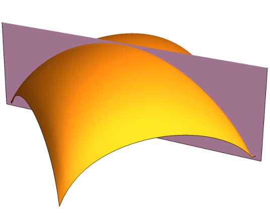
The solution set of $Q(a,b;t)=0$ is numerically plotted in Figure 4.1. The case $a=b$, shown here as a vertical plane in gray, has been discussed in Section 2. The case $a<b$, as well as our main theorem, follows from the continuity of $Q$ in $t$, and the following proposition.

The remainder of this section is devoted to the proof of this proposition.

We begin by analyzing the limit $t\to b+$.

Now we turn to the limit $t\to\infty$, which is more amusing.

Before ending this section, we propose the following uniqueness conjecture based on numeric experiments:

By definition, the two families $\mathrm{oD}\subset\mathcal{M}$ and $\mathrm{o\Delta}\subset\mathcal{N}$ are disjoint in $\mathcal{D}$. However, we will show in this section that the closure $\overline{\mathrm{o\Delta}}$ intersects $\mathrm{oD}$, and give an explicit description of the intersection in terms of elliptic integrals. This result is not strictly needed for this paper, but gives insight into the nature of the bifurcation locus.

To make this precise, we use on $\mathcal{D}$ the topology induced by the space of possible Weierstrass data, which are determined by the four real parameters $a,b,t$ and $\rho$. Clearly, the convergence of Weierstrass data implies the locally uniform convergence of the minimal surfaces.

The goal is to determine the intersection of the Meeks locus

with the closure of the non-Meeks locus

The idea is to divide the function $Q(a,b;t)$ by $b-a$ and take the limit for $a\to b$ to eliminate solutions in the Meeks locus. We claim:

Before we sketch the technical proof, we note that the function $Q$ can be extended to a holomorphic function of its arguments $a,b$ and $t$ for $a$ near $b$. To see this, note that the integrand of each of the integrals $I_{k}$ and $J_{k}$ used in the definition of $Q$ can be adjusted by multiplication with a constant factor $e^{it}$ so that the absolute values are not necessary. The square roots of the integrands cause a potential multivaluedness when the roots $-t,-a,b$ and $t$ are close to each other, which is not the case for $a$ near $b$. As $Q(a,a,t)=0$, this implies that also $\tilde{Q}$ extends to a holomorphic function of its arguments. In particular, the extension of $\tilde{Q}$ for real arguments is real analytic.

The theorem follows from the following proposition:

References

- [BF71] Paul F. Byrd and Morris D. Friedman. Handbook of elliptic integrals for engineers and scientists. Die Grundlehren der mathematischen Wissenschaften, Band 67. Springer-Verlag, New York-Heidelberg, 1971. Second edition, revised.
- [Bra92] Kenneth A. Brakke. The surface evolver. Experiment. Math., 1(2):141–165, 1992.
- [Che18] Hao Chen. Minimal twin surfaces. Exp. Math., 2018. online first.
- [ES14] Norio Ejiri and Toshihiro Shoda. On a moduli theory of minimal surfaces. In Prospects of differential geometry and its related fields, pages 155–172. World Sci. Publ., Hackensack, NJ, 2014.
- [ES18] Norio Ejiri and Toshihiro Shoda. The Morse index of a triply periodic minimal surface. Differential Geom. Appl., 58:177–201, 2018.
- [FH92] Andrew Fogden and Stephen T. Hyde. Parametrization of triply periodic minimal surfaces. II. regular class solutions. Acta Cryst. Sect. A, 48(4):575–591, 1992.
- [FH99] Andrew Fogden and Stephan T. Hyde. Continuous transformations of cubic minimal surfaces. The European Physical Journal B-Condensed Matter and Complex Systems, 7(1):91–104, 1999.
- [FHL93] Andrew Fogden, M. Haeberlein, and Sven Lidin. Generalizations of the gyroid surface. J. Phys. I, 3(12):2371–2385, 1993.
- [FK89] Werner Fischer and Elke Koch. Genera of minimal balance surfaces. Acta Cryst. Sect. A, 45(10):726–732, 1989.
- [KPS14] Miyuki Koiso, Paolo Piccione, and Toshihiro Shoda. On bifurcation and local rigidity of triply periodic minimal surfaces in , 2014. preprint, arXiv:1408.0953.
- [LHM01] Hippolyte Lazard-Holly and William H. Meeks, III. Classification of doubly-periodic minimal surfaces of genus zero. Invent. Math., 143(1):1–27, 2001.
- [Mee90] William H. Meeks, III. The theory of triply periodic minimal surfaces. Indiana Univ. Math. J., 39(3):877–936, 1990.
- [MPR98] William H. Meeks, III, Joaquín Pérez, and Antonio Ros. Uniqueness of the Riemann minimal examples. Invent. Math., 133(1):107–132, 1998.
- [MR05] William H. Meeks, III and Harold Rosenberg. The uniqueness of the helicoid. Ann. of Math. (2), 161(2):727–758, 2005.
- [PRT05] Joaquín Pérez, M. Magdalena Rodríguez, and Martin Traizet. The classification of doubly periodic minimal tori with parallel ends. J. Differential Geom., 69(3):523–577, 2005.
- [PT07] Joaquín Pérez and Martin Traizet. The classification of singly periodic minimal surfaces with genus zero and Scherk-type ends. Trans. Amer. Math. Soc., 359(3):965–990, 2007.
- [Sch90] Hermann A. Schwarz. Gesammelte Mathematische Abhandlungen, volume 1. Springer, Berlin, 1890.
- [Sch70] Alan H. Schoen. Infinite periodic minimal surfaces without self-intersections. Technical Note D-5541, NASA, Cambridge, Mass., May 1970.
- [Tra08] Martin Traizet. On the genus of triply periodic minimal surfaces. J. Differential Geom., 79(2):243–275, 2008.
- [Wey06] Adam G. Weyhaupt. New families of embedded triply periodic minimal surfaces of genus three in euclidean space. ProQuest LLC, Ann Arbor, MI, 2006. Thesis (Ph.D.)–Indiana University.
- [Wey08] Adam G. Weyhaupt. Deformations of the gyroid and Lidinoid minimal surfaces. Pacific J. Math., 235(1):137–171, 2008.