Posterior Inference for Sparse Hierarchical Non-stationary ModelsThanks: University of Cambridge, UK, Alan Turing Institute, UK
Abstract
Gaussian processes are valuable tools for non-parametric modelling, where typically an assumption of stationarity is employed. While removing this assumption can improve prediction, fitting such models is challenging. In this work, hierarchical models are constructed based on Gaussian Markov random fields with stochastic spatially varying parameters. Importantly, this allows for non-stationarity while also addressing the computational burden through a sparse banded representation of the precision matrix. In this setting, efficient Markov chain Monte Carlo (MCMC) sampling is challenging due to the strong coupling a posteriori of the parameters and hyperparameters. We develop and compare three adaptive MCMC schemes and make use of banded matrix operations for faster inference. Furthermore, a novel extension to multi-dimensional settings is proposed through an additive structure that retains the flexibility and scalability of the model, while also inheriting interpretability from the additive approach. A thorough assessment of the efficiency and accuracy of the methods in nonstationary settings is presented for both simulated experiments and a computer emulation problem.
Keywords: Gaussian Process; Multilevel models; Gaussian Markov random fields; MCMC; SPDE
1 Introduction
Gaussian processes are frequently utilised in constructing powerful nonparametric models, which are appealing due to their analytical properties. The flexibility and nonparametric nature of these models make them appropriate and useful in a wide range of applications. Gaussian process (GP) priors have been used in geostatistics (Matheron, 1973) under the name of Kriging. They are also common in other applications; for instance, in atmospheric sciences (Berrocal et al., 2010), biology (Stathopoulos et al., 2014) and inverse problems (Kaipio and Somersalo, 2006).
A large amount of research on GPs and their applications has focused on models where an assumption of stationarity for the process of interest is made. Heaton et al. (2018) provides a complete review and comparison of available methods under this assumption. Nevertheless, this assumption is rarely realistic in practice and as a consequence, several approaches to introduce non-stationarity have been proposed (Anderes and Stein, 2008; Gramacy and Lee, 2008; Kim et al., 2005; Montagna and Tokdar, 2016; Sampson et al., 2001, e.g.). Although comparative evaluations show that removing the stationary assumption improves predictive accuracy (Fouedjio et al., 2016; Gramacy and Lee, 2008; Neto et al., 2014), fitting such non-stationary models has proven to be challenging. This, combined with the well-known computational constraints of GP models, arising from storing covariance matrices, solving linear systems and computing determinants, poses important questions on how to efficiently perform Bayesian inference in non-stationary problems.
The stochastic partial differential equation (SPDE) approach introduced by Lindgren et al. (2011) employs Gaussian Markov random fields (GMRFs) to ameliorate the computational burden of working with GPs and incorporates a non-stationary framework through spatially varying parameters that are modelled as a linear combination of basis functions. Similarly, Paciorek and Schervish (2006) proposed a family of closed-form non-stationary covariance functions with spatially varying parameters modelled by a second latent GP prior. While recognised as a flexible construction, doing inference in a fully Bayesian framework becomes impractical due to the computational demands of such models. Moreover, standard Markov Chain Monte Carlo (MCMC) procedures require careful parameter tuning, exhibit mixing difficulties and require long runs to reach convergence (Neto et al., 2014; Paciorek and Schervish, 2006).
In this paper, we extend the SPDE formulation of non-stationary GPs considered by Roininen et al. (2019). This model is analogous to SPDE-based constructions in spatial interpolation (Fuglstad et al., 2015a; Fuglstad et al., 2015b; Yue et al., 2014), and to the non-stationary framework proposed by Paciorek and Schervish (2006), where the spatially varying parameters are modelled as random objects. We incorporate and account for uncertainty in the measurement noise variance and hyperprior parameters and consider two hyperpriors for the spatially varying length-scale to account for different smoothness assumptions.
The hierarchical structure of these models, that we refer to as 2-level GPs, introduces strong dependencies and hence efficient sampling from the posterior distribution is problematic. To address this, we introduce and offer a comparative evaluation of three MCMC sampling schemes. The first corresponds to an adaptive Metropolis-within-Gibbs scheme. The second employs elliptical slice sampling (ELL-SS) combined with re-parametrisations for decoupling the prior, hyperprior, and hyperparameters. The third is a marginal sampler with ELL-SS for a re-parametrised length-scale process. The developed methodology results in a non-stationary hierarchical construction that retains the flexibility of the model introduced by Paciorek and Schervish (2006) but is computationally more efficient, due to the sparse and banded structure of the finite-dimensional approximation of the precision matrix.
The 2-level models studied here naturally extend to multiple levels to construct the deep GP models of Dunlop et al. (2018). Deep GPs have received increased interest in literature and proposals differ in how the layers are combined (Blomqvist et al., 2018; Damianou and Lawrence, 2013; Dunlop et al., 2018; Hegde et al., 2019, e.g.). However, the key challenges, preventing wide-spread use of Deep GPs, include developing interpretable constructions that lack degeneracy (Duvenaud et al., 2014) and efficient and scalable inference, despite the highly coupled layers and computational expense of GPs. The hierarchical construction considered here provides an interpretable structure for nonstationary problems, as well as a sparse framework to address the computational burden, providing a promising route to deeper constructions.
Finally, extensions of the 2-level GPs to multi-dimensional settings are important and necessary in many applications. Existing approaches for two-dimensional settings are based on heavily parametrised models using spectral decompositions Neto et al. (2014); Paciorek and Schervish (2006); Risser and Calder (2017), basis function representations Katzfuss (2013), or an isotropic assumption Heinonen et al. (2016); Roininen et al. (2019). Instead, we propose a novel extension based on additive GPs (Duvenaud et al., 2011), that decomposes the function of interest in terms of low-dimensional functions, which are modelled as separable non-stationary processes. Important advantages include increased intrepretability and robustness to curse of dimensionality, while inheriting the appealing flexibility of 2-level GPs. The additive structure permits scalability, by taking advantage of the sparse banded precision matrices, low-dimensional representation, and efficient Kroneacker algebra for the separable interaction terms. Moreover, it can capture long-range structures in the data. The choice of interaction terms may be application driven, and hyperpriors can be employed to determine their importance. In this case, the MCMC schemes can be extended through a Gibbs sampling framework. This extension provide an efficient method for data-dense problems in low dimensions but also enables using the construction for multidimensional (nD) problems with relatively sparse data, similar to (Volodina and Williamson, 2018).
The paper is organised as follows. We start by summarising related work in Section 2. In Section 3, we present the sparse non-stationary hierarchical model for one-dimensional problems and describe the proposed sampling schemes in Section 4. Section 5 extends the model to multi-dimensional settings, while retaining the computational benefits and flexibility. The experiments in Section 6 provide a complete empirical evaluation, with a study of the discretisation and sample size effects and performance for different signal types, as well as a comparison with alternative GP models. Finally, Section 6.4 applies the methodology to a computer emulation problem for a NASA rocket booster vehicle.
2 Related work and background
We begin with a review of Gaussian process models, providing a connection between the non-stationary GPs of Paciorek and Schervish (2006) and the SPDE formulation in Lindgren et al. (2011) and Roininen et al. (2019).
2.1 Gaussian process models
Let us denote by noisy realisations of an unknown random process . A standard GP regression model assumes
| (2.1) |
where is zero-mean Gaussian noise with variance and a Gaussian process. More precisely, the model can be written in a hierarchical form,
| (2.2) |
where is a covariance function parametrised by and must define a valid covariance matrix (symmetric and positive semi-definite). The covariance function encodes important properties of the process, such as its variation and smoothness. Stationary covariance functions only depend on the inputs through and are most often the default choice. Typical covariance functions include the stationary squared exponential (SE),
| (2.3) |
and the stationary Matérn family, formulated as
| (2.4) |
where is the gamma-function, is the smoothness parameter, is the length-scale, is the magnitude or variance parameter, and denotes the modified Bessel function of the second kind of order .
However, the translation-invariance assumption of stationary covariance functions may be inappropriate for certain applications where the process is spatially dependent, such as, for problems in environmental, geospatial and urban sciences. In these cases, a non-stationary formulation of the model is desirable. Paciorek and Schervish (2006) introduced a family of non-stationary covariance functions,
where is a stationary correlation function on ; is a spatially varying covariance matrix, referred to as a kernel matrix, which describes local anisotropies; and
The non-stationary version of the Matérn covariance function is therefore,
| (2.5) |
with hyperparameters . When employing this type of non-stationary covariance function in equation (2.2), we are required to infer the kernel matrices at every location where the process was observed. Paciorek and Schervish (2006) modelled the kernel matrices as a continuous-parameter random process by utilising its spectral decomposition. Nonetheless, this approach results in computationally expensive inference (Paciorek and Schervish, 2006, Section 5.1) even for one-dimensional problems. As a consequence, alternative approaches to model the spatially varying parameters have been proposed (Lang et al., 2007; Neto et al., 2014; Risser, 2016).
We note that for one-dimensional problems, the kernel matrices, , are reduced to scalars, which we denote as . In this setting, when modelling the spatially varying length-scale with a GP, the hierarchical formulation of the model is
| (2.6) |
where is as in equation (2.5) and is a stationary covariance function with parameters . We note that the prior for the spatially varying length-scale is assigned over a transformed parameter, defined as , with representing the a priori constant mean of the log length-scale process.
Efficient sampling from the posterior is challenging and the computational burden introduced by the spatially varying parameter is noticeable even in one-dimensional problems (Heinonen et al., 2016; Paciorek and Schervish, 2006). These difficulties arise from different sources. First, the computational complexity inherited from dense covariance matrices makes the model unsuitable for large datasets. Second, the latent processes and hyperparameters tend to be strongly coupled, leaving vanilla MCMC schemes inefficient. Finally, as in a stationary formulation, the model is sensitive to the choice of hyperparameters, , and therefore these must be inferred (Neto et al., 2014).
2.2 SPDE formulation of Matérn fields
Lindgren et al. (2011) showed that Gaussian Markov random fields can be presented equivalently as stochastic partial differential equations. By fixing , a GP with stationary Matérn covariance (2.4) and a Markov property can be defined through
| (2.7) |
where is the Laplace operator, is white noise on , and
Analogous to the construction of Paciorek and Schervish (2006) for non-stationary covariance functions with spatially varying length-scales, Roininen et al. (2019) derive an SPDE formulation for non-stationary Matérn fields,
| (2.8) |
where is a spatially varying length-scale, that is modelled as a log-transformed continuous-parameter GP in the hyperprior in equation (2.6). An alternative formulation was proposed by Lindgren et al. (2011, Section 3.2), where spatially varying parameters were modelled through a basis function representation. Such a choice gives computational advantages, through a lower dimensional parameter space. However, this requires selecting the number of basis functions, and the ability to flexibly recover changes in the length-scale strongly depends on this choice.
A finite-dimensional approximation of our continuous-parameter model (2.8) can be written in vector-matrix format as where is a sparse matrix depending on , with denoting the discretisation step in a chosen finite difference approximation. This model is constructed in such a way that the finite-dimensional approximation converges to the continuous-parameter model (2.8) in the discretisation limit (for proofs, see Roininen et al. (2019)). This property guarantees that irrespective of the choice of , the posteriors, and hence also the estimators, on different meshes, that are dense enough, are essentially the same.
The SPDE formulation in (2.7) considers periodic boundary conditions, which can lead to undesirable effects in the edges of the estimators. In order to correct a possible boundary effect, one can add points around the boundary. This domain extension offers also a possible benefit in the sparse structure of . By construction, the matrix is a cyclic tridiagonal matrix, and while Sherman-Morrison formula can be applied to solve this type of systems efficiently (e.g. Seiler and Seiler (1989)), we can simply neglect the matrix elements in the corners once we have applied domain extension and take advantage of the resulting tridiagonal structure.
We note that employing a GP to model results in a similar construction to that discussed in Section 2.1. In the next sections, we extend the work of Roininen et al. (2019), by including inference of the measurement noise variance and the length-scale hyperparameter. Additionally, we explore different hyperprior models, discuss MCMC algorithms to do inference with these types of models, and present an efficient way to extend the model to higher dimensions.
3 Sparse non-stationary hierarchical models
The GP formulation in equation (2.1) can be rephrased through
| (3.1) |
where represents a linear mapping from some function space to a finite-dimensional space and is assumed to be zero-mean Gaussian noise with variance , which is independent of . For computational reasons, we discretise this equation, such that , obtaining the right hand side of equation (3.1), where is a known matrix and with . In this case, through the matrix , we are able to define the grid resolution of the latent fields. In particular, for more rough processes, we may be interested in finer resolutions, while for smooth functions, a sparse grid may be sufficient to obtain an accurate representation.
Our aim is to decompose the inverse covariance matrix , where is a sparse matrix that depends on the log length-scale parameters . The required decomposition can be achieved employing the SPDE approach from Section 2.2. An explicit hierarchical formulation of the model is
| (3.2) |
where denotes the -dimensional vector with all elements equal to . As both the length-scale and magnitude parameters cannot be estimated consistently (Zhang, 2004), we use the observe data to set the magnitude and mean of both the stationary and non-stationary processes to improve identifiability, with full details provided in the Supplementary Material. The key component of the model is , the inverse covariance of the GMRF employed to represent the non-stationary GP. This precision matrix depends on , which is assumed to be a constant-mean GP that describes the spatially varying log length-scale, and denotes the length-scale parameter of the covariance function that describes the properties of the log length-scale process. A plate diagram of this model is given in Figure 1 (left).
2-level GP
3-level GP
: observed data
: noise variance
: non-stationary process
: variance of
: log length-scale process
: mean of
: variance of
: log length-scale process
: mean of
: variance of
: length-scale
In the following, we discuss different types of hyperpriors for . Notice that we are free to assign an inhomogeneous Matérn field for the log length-scale process, introducing more flexibility to the model. A graphical representation of this type of 3-level construction is given to the right of Figure 1. For simplicity, we focus on the 2-level case, when the parameters of the log length-scale process are restricted to be constant along the input space.
AR(1) hyperprior.
A hyperprior with sample paths smoother than white noise is needed, otherwise different discretisations of may affect the posterior estimates (Roininen et al., 2019). One such process is the Ornstein-Uhlenbeck, a member of the stationary Matérn family (equation (2.4)), with exponential covariance function obtained by setting . The Ornstein-Uhlenbeck has non-differentiable sample paths, allowing quick changes in the behaviour of the log length-scale process. It is the continuous-time counterpart of the first-order autoregressive model AR(1) given by and , where is on an uniform lattice , with discretisation step . Without a proof, we note that the AR(1) has an exponential autocovariance for all except for which corresponds to Gaussian random walk, i.e. Brownian motion. While the stable AR(1) requires that , this is not a necessary condition here, as our goal is in forming covariance matrices. Let us denote by and . Then, we can construct the inverse of the exponential covariance matrix , where is a sparse matrix that depends on and . More precisely, is a banded matrix, with nonzero elements only on the main diagonal given by and the first diagonal above this given by . The coefficients are defined as
Hence, we have a sparse representation for the hyperprior precision matrix, and the banded structure in offers important computational advantages when evaluating , as the required determinant computations, matrix multiplications, and system of equations can be significantly simplified.
SE hyperprior.
In contrast to the AR(1) hyperprior, we have the squared exponential hyperprior (equation (2.3)) for . This covariance function, also referred to as the radial basis function (RBF), is recovered when in the stationary Matérn covariance of equation (2.4). Sample paths from a SE are infinitely differentiable and consequently very smooth. Therefore, when employing a SE hyperprior for the length-scale process, we introduce strong prior smoothness assumptions on how the correlation of the non-stationary process changes with distance. We note that for the SE hyperprior, the precision matrix is dense and therefore, comes at an increased computational cost.
4 Inference for one-dimensional problems
In order to efficiently draw samples from the posterior distributions of interest, we explore three MCMC sampling approaches. The first draws samples from the multidimensional vector through an adaptive Metropolis-within-Gibbs algorithm. The second employs ancillary augmentation (Yu and Meng, 2011) over and and uses elliptical slice sampling (Murray et al., 2010, ELL-SS,) over the re-parametrised log length-scale process. The third integrates out the non-stationary process, resulting in a marginal sampler that draws from by combining ancillary augmentation and ELL-SS to break the correlation between and .
4.1 Metropolis-within-Gibbs (MWG)
This sampling scheme is inspired by that proposed in Roininen et al. (2019) and additionally incorporates adaptive random walks (Roberts and Rosenthal, 2009) for the noise variance, length-scale hyperparameter, and log length-scale process. The procedure is detailed in Supplementary Algorithm 1.
The MWG framework updates the log length-scale process at each location individually and, regardless of the hyperprior employed, offers computational gains due to the fact that when proposing a single element of the log length-scale process , for , the -ratio of the prior density of used in the acceptance probability simplifies to
Here is the proposed log length-scale vector, obtained by updating the th element of to , and combined with pentadiagonal form of the precision matrix, resulting from multiplication of tridiagonal matrices , the computational complexity of the quadratic term in the -ratio is reduced from to . Moreover, the -determinant can be computed through numerically stable and inexpensive operations; for details, see Roininen et al. (2019, Section 6). Similarly, the -ratio of the prior density of simplifies to
where denotes the element of the matrix . Further computational gains are possible when we utilise the AR(1) hyperprior, as the tridiagonal form , resulting from the sparse AR(1) construction of , reduces this operation from to .
Additionally, when proposing a new hyperparameter , we must evaluate
For the SE hyperprior, this requires the inversion of a dense matrix, while the tridiagonal form of for the AR(1) hyperprior makes this considerably cheaper by reducing the computational complexity of this -ratio term from to . In addition, our simulation studies show that this algorithm does not perform well when the hyperprior for has strong smoothness assumptions, such as those induced by employing a SE covariance function. This flaw motives us to explore alternative algorithms.
4.2 Whitened elliptical slice sampling (w-ELL-SS)
Elliptical slice sampling is a state-of-the-art MCMC algorithm for latent Gaussian models (Murray et al., 2010). Here, we combine this sampling algorithm with ancillary augmentation or whitening (Yu and Meng, 2011), which represents a computationally cheap and effective strategy to break the correlation between the prior and its corresponding hyperparameters (Filippone et al., 2013; Murray and Adams, 2010).
We can equivalently define the unknown function as with and the log length-scale vector as with . For the AR(1) hyperprior, ; whereas, for the SE hyperprior, we define to be the lower-triangular Cholesky factor of . Re-parametrising in terms of the whitened parameters and , results in the joint posterior
The sampling method is described in Supplementary Algorithm 2. As opposed to the MWG, the log length scales are updated jointly through the whitened parameter . In this case, the likelihood can be evaluated as a product of univariate Gaussian distributions, after computing and solving . Regardless of the hyperprior employed, the latter system of equations can be solved in operations by taking advantage of the tridiagonal structure of (Rue and Held, 2005). The former system of equations requires matrix multiplication, resulting in operations; however, for the AR(1) hyperprior, we can equivalently solve and make use of the banded form of to reduce this to operations.
Thus, while MWG requires looping over the elements of the -dimensional log length-scale vector, with each operation costing operations for the AR(1) hyperprior and operations for the SE hyperprior, the w-ELL-SS instead updates this vector jointly through for the AR(1) hyperprior and operations for the SE hyperprior. However, as ELL-SS is a rejection free sampling method, each iteration may require several likelihood evaluations, mitigating any gain in computation time of this scheme.
4.3 Marginal elliptical slice sampling (m-ELL-SS)
In simulation studies, we found that integrating out the unknown function significantly improves the mixing of and its hyperparameters. The marginal likelihood of the data corresponds to
| (4.1) |
where . Again, we use whitening to decouple and , with the re-parametrisation and for the AR(1) hyperprior or for the SE hyperprior. The posterior is
The sampling scheme is detailed in Supplementary Algorithm 3. Again, the log length scales are updated jointly through the whitened parameter . This requires first computing , an operation for the AR(1) hyperprior and operation for the SE hyperprior. However, in comparison with the w-ELL-SS, which proceeds by solving and simply taking the product of univariate Gaussians in operations, we must evaluate the marginal likelihood in (4.1).
When computing the marginal likelihood, we emphasise that the required calculations for can be computed employing the Woodbury identity;
While this identity also requires a matrix inversion, note that is also banded and therefore computations are considerably cheaper. Indeed, the quadratic term in the marginal likelihood (4.1) is
with the most expensive operation of order . Specifically, the first term can be computed in operations, while the second term can be efficiently computed by breaking it into three separate operations. First, we set , with computational complexity reduced from to through sparsity in . Next, we solve in operations due to the banded form of the matrix. Finally, we compute , with a cost of operations. Computing the determinant, on the other hand, is more expensive with the dominant term costing or , whichever is greater. Specifically, we must first solve , with complexity , and then compute , with reduced complexity due to sparsity in . Finally, the determinant of the matrix is computed.
In addition, when proposing new values for the noise variance or the length scale , we must recompute the marginal likelihood (4.1), as opposed to evaluating the product of univariate Gaussians for the w-ELL-SS scheme, increasing the cost of these steps as well. However, in the marginal scheme, in contrast to both MWG and w-ELL-SS, sampling of is no longer required. We also note the computational gains of the AR(1) over the SE hyperprior deteriorate when the determinant evaluation dominates this computation, i.e. when .
The increased computational cost of the marginal scheme comes with improved mixing, and this trade-off is examined in the simulation studies of Section 6.3. In contrast to MWG, this scheme performs well regardless of the hyperprior employed.
5 Extensions for -dimensional problems
To extend the model from Section 3 to higher dimensional settings, while maintaining its computational benefits, a novel construction is proposed utilising additive Gaussian process models (Duvenaud et al., 2011, AGP,). First, the model is presented, followed by a description of the extended inference procedure.
5.1 Sparse non-stationary additive models
Additive regression models decompose the regression function into main effects and interactions. Linear regression is a classic example, and nonparametric additive models (Friedman and Stuetzle, 1981; Buja et al., 1989) provide increased flexibility, while retaining interpretability and robustness to the input dimension, when compared with general nonparameteric surfaces. The additive GP formulation results from considering the sum and product of covariance functions, two operations for constructing valid covariance functions in -dimensions. This provides a flexible and interpretable model for the unknown function to include main first-order terms up to -order interaction terms, assumed to be separable across dimensions.
In the additive GP, the choice between low-order and high-order terms represents a trade-off between between interpretability and accuracy. On one hand, by including only first-order terms, the model can capture long-range structures and has increased intrepretability. On the other, including only a -order separable function increases flexibility and complexity. Duvenaud et al. (2011) include all iteration terms and develop a maximum marginal likelihood approach to determine the importance of each term. Additionally, they develop an efficient algorithm, despite the exponential number of terms, through parametrisations that limit the number of hyperparameters. Interestingly, their experiments show that typically only a few orders of interactions are important. Alternatively, the choice of terms in the additive GP may be application driven; more recently, this is the approach taken in Cheng et al. (2019) for longitudinal biomedical data. Another interesting direction in Gilboa et al. (2015) constructs projected additive GPs through first-order functions of linear projections of the inputs.
For notational simplicity, in the following, we focus on the 2-dimensional setting, including both the main and interaction terms for generality. The model construction and inference can be applied to -dimensional settings, through appropriate choice of the terms to include in the additive formulation. In two-dimensional problems, the discretisation is based on a complete grid, with the noisy realisations modelled through
where , and are known matrices. We assume and are independent one-dimensional non-stationary processes, while is a two-dimensional, separable non-stationary process. Thus, denotes the vector formed by the first-order non-stationary processes at the locations in dimension , while collects the second-order non-stationary process at all locations on the complete grid.
The hierarchical structure of the model (depicted in Figure 2) is
| (5.1) |
with . In equation (5.1), we have four one-dimensional length-scale processes: two describing the correlation changes in each direction independently and two incorporating that information in a two-dimensional process, through a separable assumption A visualisation of the non-stationary additive covariance function is provided in Supplementary Figure S1.
: observed data
: noise variance
: 1st order non-stationary processes
: 2nd order non-stationary processes
: 1st order log length-scale processes
: 2nd order log length-scale processes
: length-scales
Because the AGP is based on one-dimensional kernels, we can directly apply the methodology discussed in Section 3 for any of the hyperpriors studied. Instead, a direct extension of the SPDE model to two-dimensional settings will not allow us to employ the AR(1) hyperprior and benefit from its computational advantages. This is because a two-dimensional exponential covariance does not have a valid Markov representation. Furthermore, the additive and hierarchical structure of the model in equation (5.1) favours interpretability about the behaviour of the correlation in each dimension.
5.2 Inference for additive non-stationary models
The posterior for the additive non-stationary model in equation (5.1) is
with being a separable covariance matrix, defined as , where denotes the Kronecker product. The three inference schemes described in Section 4 can be appropriately extended through a blocked Gibbs sampler, that updates the three blocks of parameters ; ; and from their full conditional distributions. Following from the one-dimensional synthetic experiments of Section 6.1, we focus on the marginal sampler of Section 4.3. We will refer to it as the block marginal elliptical slice sampler (Block-m-ELL-SS); in this case, although we are not integrating out the processes , we use the marginal likelihood to sample the length-scale process and corresponding length-scale hyperparameters in each block. For instance, when sampling the block , the full conditional factorises as
with denoting the whitened parameter. Thus, we first sample from the block marginal utilising the steps described in Section 4.3, with the marginal likelihood replaced by . The algorithm is detailed in Supplementary Algorithm 4. For efficiency in evaluating the block marginal likelihood obtained from integration of , , the matrix determinant lemma (Harville, 1997) must be employed to avoid computing the determinant of an matrix and instead evaluate the determinant of three small matrices.
When an interaction term is employed in the model, the algorithm requires samples from the posterior of , which is a Gaussian distribution with mean and variance . These posterior moment computations need the inversion of an matrix and cannot exploit the Kronecker structure because of the second summand in . To overcome this, we utilise the efficient method of Gilboa et al. (2015, Section 2.2), based on eigendecompositions and matrix-vector multiplications for Kronecker matrices. This procedure applies to the case when ; this constraint requires the data to be observed on the complete grid (not necessarily equidistant), but can easily be relaxed for incomplete grids and domain extensions with an additional Gibbs step to sample the missing observations. Specifically, we make use of the identity
| (5.2) |
where and , with and denoting the eigenvectors matrices and and denoting the diagonal matrices of eigenvalues of and , respectively. The second key identity is
| (5.3) |
where the operator returns a matrix whose elements are taken from the vector , and denotes the vectorisation of a matrix .
Thus, to efficiently compute the posterior mean, , we follow three steps:
where . Note that is diagonal and therefore easy to invert. A posterior sample of is then obtained by sampling and setting , where for the latter operation, we again make use of the second identity (5.3) and the diagonal form of .
The last critical computation is the evaluation of the block marginal likelihood , which is required to sample and the corresponding hyperparameters, and . First, the quadratic term can be calculated efficiently following the approach employed for the posterior mean. Next, for the determinant computation, one can use again the eigendecomposition; namely,
where is a diagonal matrix, whose determinant is straightforward to calculate. We emphasize the required terms can also be efficiently computed for higher-order interactions through -dimensional versions of the two key identities (5.2) and (5.3) in Gilboa et al. (2015).
6 Experiments
We apply the sparse non-stationary hierarchical methodology to three simulated 1-dimensional interpolation experiments and a two-dimensional synthetic example. First, the one-dimensional experiments study the effects of the discretisation and sample size on the efficiency of the algorithms presented in Section 4 under two extreme hyperpriors. In addition, the experiments show that our model can recover different signal types, while also providing information on the correlation structure. Second, a two-dimensional synthetic experiment demonstrates how the model can be extended to higher dimensions utilising an AGP model. Finally, in Section 6.3, we present a comparative evaluation on the performance of 2-level GP models against two other methods: a stationary GP model and a Bayesian treed GP (Gramacy, 2007, TGP,) model, a popular approach for dealing with non-stationarity.
6.1 One-dimensional synthetic data
We consider three simulated datasets with different signal types. The first example (Supplementary Figure S2a) is a function with smooth parts and edges and is also piecewise constant. The second synthetic dataset (Supplementary Figure S2b) is a damped sine wave function with smooth decaying oscillations. The third example corresponds to the Bumps (Supplementary Figure S2c) function employed by Donoho and Johnstone (1995), which depicts a signal with pronounced spikes and constant parts. In the first dataset, we investigate, empirically, posterior consistency of the estimates with respect to the discretisation scheme. The second experiment explores the performance of the sampling schemes for increased sample size and measurement noise. The last example examines emphasises the importance of the prior choice.
Experiment 1: Smooth-piecewise constant function
For all experiments, we use the same initialisation and run the chains for iterations. The burn-in period is algorithm specific, selected according to preliminary runs based on Raftery and Lewis’s diagnostic (Raftery and Lewis, 1992) for the second level length-scale. Numerical discretisation-invariance is studied by varying in the experiments, with . The mean and variance of the prior length-scale process is set at zero and one, respectively. For the second level length-scale, we use a broad prior, .
We start by presenting the results obtained with the MWG algorithm. Figure 3 shows estimates of the spatially varying length-scales and the unknown function under both hyperpriors. For the AR(1) hyperprior, an inspection of traceplots and cumulative averages of the estimates (not shown) suggest convergence of the chains for all discretisation schemes. In addition, the varying length-scale estimates exhibit the expected behaviour (i.e. decaying when the function has a sharp jump and increasing when the function is constant), and the interpolated estimates indicate a reasonable fit to the unknown function for all three discretisations schemes (Figure 3-). However, this is not the case for the SE hyperprior. Figure 3- illustrates the results obtained with this hyperprior for the same sampling algorithm. Under this setting, the effect of discretisation scheme is evident. As we increase , the method fails to recover the unknown function. The strong correlation between the elements of induced by the SE hyperprior makes the algorithm converge rather slowly to the target distribution.
In contrast to the results obtained with MWG, both w-ELL-SS and m-ELL-SS demonstrate convergence for both hyperpriors and invariance to the discretisation (see Supplementary Figures S3 and S4 for a complete analysis). Figure 4 summarises succinctly important differences in mixing across the algorithms by showing traceplots with cumulative averages for a subset of parameters. The results are shown for the most challenging scenario, SE hyperprior at the highest resolution, . Figure 4 emphasises the lack of convergence for MWG. Figure 4 demonstrates the high autocorrelation of the chains and the slow convergence produced by w-ELL-SS. Finally, Figure 4 highlights the improvement offered by m-ELL-SS, fast convergence to the stationary distribution and low autocorrelation of the chains.


In order to evaluate the performance of the algorithms, we show in Table 1 an overall efficiency score (OES) of the chains (Titsias and Papaspiliopoulos, 2018). This measure considers both the CPU time (Supplementary Table S2) required to run the chains and the effective sample size (ESS) (Supplementary Table S3). The score is computed as 11 1 All experiments were run in an Intel Core i7-6700 CPU (3.40GHz, 16 GB of RAM).. For both multidimensional vectors, and , we report the OES computed with the minimum ESS across all dimensions. The results indicate that while MWG with the AR(1) hyperprior shows high efficiency for some parameters when , its performance deteriorates as increases. This suggests that this sampling scheme will not perform efficiently for bigger datasets even when (this is explored in Experiment 2). Furthermore, despite the fact that MWG reports the lowest CPU time under the AR(1) hyperprior (Supplementary Table S2), its overall efficiency scores are outperformed by those obtained with m-ELL-SS; this is due to the low autocorrelation of the chains achieved by the marginal sampler (see Supplementary Table S3). In contrast, chains of the parameters for w-ELL-SS result in the worse OES. Notice also that the scores reported for MWG with the SE hyperprior are not informative as the chains show convergence problems. Table 1 also reports mean absolute error (MAE) to evaluate the fit to the unknown function and the empirical coverage of the credible intervals (EC) to evaluate accuracy in uncertainty quantification. For the SE hyperprior, w-ELL-SS and m-ELL-SS report equivalent errors and EC, while MWG yields worse values.
| MWG | w-ELL-SS | m-ELL-SS | ||||||||
|---|---|---|---|---|---|---|---|---|---|---|
| AR(1) | 622.76 | 173.12 | 65.99 | 380.89 | 102.38 | 38.91 | 661.20 | 257.81 | 116.35 | |
| 635.36 | 114.02 | 41.05 | 30.90 | 8.99 | 2.94 | 287.16 | 114.36 | 59.71 | ||
| 203.80 | 42.10 | 13.91 | 9.12 | 2.34 | 0.86 | 129.75 | 52.16 | 22.30 | ||
| 89.84 | 15.66 | 6.00 | 22.77 | 5.26 | 2.36 | 111.80 | 45.54 | 21.53 | ||
| MAE | 0.041 | 0.051 | 0.054 | 0.041 | 0.051 | 0.054 | 0.041 | 0.051 | 0.053 | |
| EC | 0.988 | 0.975 | 0.971 | 0.988 | 0.975 | 0.975 | 0.988 | 0.975 | 0.975 | |
| SE | 11.19 | 4.88 | 7.49 | 246.24 | 77.72 | 8.89 | 856.15 | 253.91 | 125.97 | |
| 1.22 | 0.73 | 0.64 | 21.69 | 10.22 | 2.79 | 244.91 | 122.57 | 55.82 | ||
| 0.06 | 0.01 | 0.01 | 4.71 | 1.37 | 0.24 | 76.80 | 24.11 | 9.87 | ||
| 0.59 | 0.75 | 0.31 | 2.31 | 0.29 | 0.01 | 16.59 | 4.15 | 2.21 | ||
| MAE | 0.078 | 0.100 | 0.133 | 0.040 | 0.050 | 0.054 | 0.039 | 0.049 | 0.052 | |
| EC | 0.889 | 0.826 | 0.763 | 0.988 | 0.975 | 0.971 | 0.988 | 0.975 | 0.979 | |
Experiment 2: Damped sine wave
This example explores the effect of increasing the sample size and measurement noise. Due to robustness of the estimates with respect to the discretisation in the first example, we only present experiments for the discretisation scheme when . The chains are run for iterations with a burn-in period that is algorithm and prior specific. In addition, we extend the domain with points on each side of the interval, such that and . The prior distributions for and are as in Experiment 1.
| AR(1) | SE | |||||
| MWG | w-ELL-SS | m-ELL-SS | MWG | w-ELL-SS | m-ELL-SS | |
| 12.73 | 27.54 | 14.21 | 0.27 | 32.29 | 15.27 | |
| 0.06 | 0.14 | 0.65 | 0.00 | 0.40 | 1.04 | |
| 0.13 | 0.13 | 0.75 | 0.01 | 0.55 | 1.41 | |
| 0.19 | 0.36 | 0.95 | 0.02 | 0.05 | 0.25 | |
| MAE | 0.038 | 0.039 | 0.039 | 0.089 | 0.038 | 0.038 |
| EC | 0.920 | 0.934 | 0.934 | 0.863 | 0.940 | 0.934 |
While the results with the AR(1) hyperprior appear satisfactory under the three sampling schemes (Supplementary Figure S5), once again, SE hyperprior (Figure 5) with MWG is not able to explore the posterior of , resulting in poor estimates and hence, the highest MAE and poor EC (see Table 2). Analysing the efficiency of the samplers, first, for the AR hyperprior, we observe that while MWG is faster (Table S4), its ESS is consistently smaller (Supplementary Table S6), hence reducing its OES (Table 2). In contrast to the findings in Experiment 1, w-ELL-SS reports better OES compared to MWG due to better mixing in the chains. We believe this is due to the noise level, which favours a whitened parametrisation. Finally, despite the fact that the marginal sampler reports larger CPU times, the low correlation of its chains (Supplementary Table S6) favours its OES. Second, when using the SE hyperprior, the marginal sampler appears to be significantly faster and consistently reports the best OES. This, together with the negligible differences in MAE and EC, suggests that m-ELL-SS offers a good compromise between computational cost and efficiency, with the benefit of working well under highly correlated priors.
Experiment 3: Bumps
The data is generated employing the Bumps function in Donoho and Johnstone (1995) and scaled to have zero mean and unit variance. Following Vannucci and Corradi (1999), we generate points in the interval [0,1] and use a signal-to-noise ratio equal to 5, such that . To avoid a boundary problem, we extend the domain with points on each side of the interval, such that . Chains are run for iterations with algorithm and prior specific burn-in periods. We use empirical priors for the length-scale process and length-scale hyperparameter; namely, , , and (see Supplementary Section E.3.1 for more details on prior elicitation).
This example highlights important differences between the two hyperpriors and the proposed MCMC algorithms. First, under the AR(1) hyperprior, the three sampling schemes show differences in the posterior length-scale process (Figure 6-). While MWG results in a smooth process, m-ELL-SS and w-ELL-SS appear to be more sensitive to the prior, with rougher estimates. Second, for the SE hyperprior, once more, MWG did not reach convergence. Also, the performance of w-ELL-SS has become impaired; the posterior length-scale process does not reflect the changes in the correlation structure, and the length-scale hyperparameter did not reach the stationary distribution. The posterior length-scale process obtained with m-ELL-SS appears more appropriate, although, still shows a prior effect.
| AR(1) | SE | |||||
| MWG | w-ELL-SS | m-ELL-SS | MWG | w-ELL-SS | m-ELL-SS | |
| 23.42 | 5.73 | 5.70 | 2.06 | 5.48 | 15.36 | |
| 0.01 | 0.01 | 0.13 | 0.00 | 0.01 | 0.15 | |
| 2.43 | 0.10 | 0.24 | 0.56 | 0.07 | 0.85 | |
| 0.65 | 0.03 | 0.13 | 0.07 | 0.00 | 0.03 | |
| MAE | 0.060 | 0.061 | 0.062 | 0.461 | 0.069 | 0.060 |
| EC | 0.955 | 0.950 | 0.959 | 0.385 | 0.961 | 0.967 |
The findings discussed above are also evidenced in the OES shown in Table 3, where MWG exhibits the highest scores and the lowest MAE under AR(1). In contrast, the m-ELL-SS scheme outperforms MWG and w-ELL-SS for a SE hyperprior. We believe the differences illustrated in this experiment are a result of a key challenge of elliptical slice sampling. When the likelihood is strong, the sampler can result in poor mixing and, in extreme cases, can get stuck (Fagan et al., 2016). In addition, when sampling kernel parameters in strong likelihood settings, one can expect a non-centred parametrisation (avoiding whitening) to be more efficient (see Section 3 in Murray and Adams (2010)).
The computational time required for this experiment is reported in Supplementary Table S9. Given the same initial values, the marginal sampler converges to the stationary distribution faster; indeed, m-ELL-SS reports, across experiments, the smallest time spent in burn-in period. Finally, to highlight how the model can benefit from using a more powerful computer, we ran this experiment in an Intel Xeon E5-260V3 2.4GHz (Haswell), 8-core processors with 4GB per core, and we found that the inference procedure is sped up by a factor of for m-ELL-SS and w-ELL-SS (see Supplementary Table S10). However, for MWG, the speed up factor was only .
6.2 Two-dimensional synthetic data
We study the performance of our approach on a - synthetic dataset, by generating noisy observations in an expanded grid of equally spaced points in , employing , where both and correspond to the function used in Experiment 1. The noise variance is set to and the sampler is run for iterations, with a burn-in of . We use the same prior distributions of Experiment 1 for each of the length-scale processes and corresponding hyperparameters.
Figure 7 depicts the true surface versus the posterior mean obtained from a 2-level AGP model (without interaction term), employing the Block-m-ELL-SS algorithm. Our model is able to capture the smooth areas and edges of the surface. In addition, it provides information about the correlation structure along each axis (Figure 7). The 2-level AGP correctly learns the varying correlation along the surface; for instance, the true function in the region is constant, and in the same region, the 1- length-scale processes depict strong correlation. The required total computational time for this experiment was 99.26 minutes (19.67 in burn-in and 79.59 in non-burned).
6.3 Comparative evaluation
We offer a comparative evaluation of our model for the synthetic examples from Section 6.1 and 6.2, against: 1) stationary Mátern Gaussian process (STAT) with and 2) Bayesian treed Gaussian process (TGP). For the stationary model, the length scale and noise variance are inferred via MCMC, employing a marginal sampler with adaptive random walks. The GP prior mean and magnitude are fixed at and , respectively, as in the 2-level GP model. For the TGP, we consider a stationary Matern kernel with and a constant mean function. The magnitude is also inferred, in contrast to the stationary and the 2-level model. In order to make use of the default prior distributions, we rescale the response and inputs, as recommended by the authors.
In all the experiments, the chains are run for the same number of iterations (), with the same burnin period (), and initialised with the same values for STAT and 2-level GP. For our two-dimensional simulated dataset (Experiment 4), we were unable to run the TGP model22 2 A single iteration of TGP took more than 24 hours on an Intel Core i7-6700 CPU (3.40GHz, 16 GB of RAM). Also, we used TGP in an iMac Pro (2.3GHz 18-core Intel Xeon W processor, Turbo Boost up to 4.3GHz, 128GB 2666MHz DDR4 ECC memory) and after 2 weeks, the code was still running., due to the size of the dataset. To offer a comparison, we consider a subset of the original data, reducing the data size from to observations.
Figure 8 shows the posterior mean estimates of the unknown under the three models for the three different 1- synthetic datasets, and Figure 9 illustrates the posterior mean surface for the subset of data in Experiment 4. In addition, Table 4 reports MAE and EC of the experiments. Note that the grey areas depict the credible intervals of the unknown function for STAT and 2-level GP but, instead, depict the credible intervals of the noisy observations for TGP. This is because storing region-specific traces is memory intensive, and the storage is not supported in the tgp package without doing predictions. Similarly, we report EC of the noisy process for TGP in Table 4.


| STAT | TGP | 2-level GP (AR/SE) | |||||
|---|---|---|---|---|---|---|---|
| m | MAE | EC | MAE | EC⋆ | MAE | EC | |
| Experiment 1 | 81 | 0.076 | 0.914 | 0.056 | 0.963 | 0.041/0.039 | 0.988/0.988 |
| Experiment 2 | 350 | 0.047 | 0.946 | 0.043 | 0.934 | 0.039/0.038 | 0.934/0.940 |
| Experiment 3 | 512 | 0.094 | 0.947 | 0.079 | 0.963 | 0.062/0.060 | 0.959/0.967 |
| Experiment 4 (subset) | 441 | 0.195 | 0.501 | 0.122 | 0.980 | 0.072 | 0.963 |
First, the results make clear the downside of applying a stationary model to non-stationary data in all four experiments. In Experiment 1, STAT is oversmoothing and unable to capture the edges in the function (see Figure 8). Example 2 and 3 (Figures 8) illustrate how a stationary model tends to overfit when the function is constant, as a result of the different characteristics of the unknown. The same behaviour is repeated in the two-dimensional synthetic example (Figure 9).
Second, while TGP offers an improvement, compared with a stationary setting, the model still oversmooths where the function possesses an edge. For instance, in Figure 8, the partition found around is misplaced, and a third partition should be included around to capture correctly the edges. In Experiment 2 (Figure 8), the partition is also misplaced; this is however more reasonable (compared to Experiment 1) due to the smooth change in the behaviour. In Experiment 3, despite the fact that TGP fit is good when the function is constant (Figure 8), the main limitation appears to be in finding some of the partitions that are required to ameliorate the issues resulting from fitting piecewise stationary models. Note that we ran TGP with a different number of iterations (; and ) to verify the results shown in Figure 8 and 9 (see Supplementary Section F for the results). In Experiment 3, while increasing the number of iterations has a positive effect on the partitions found (and therefore on MAE), it was not enough to outperform the 2-level GP model. Also, this was not the case for the other experiments, where increasing the number of iterations either did not affect the fit or worsened it. Moreover, without knowing the ground truth, it would be hard to know beforehand if the algorithm has been run for long enough to find the appropriate partitions.
In summary, the 2-level GP is an alternative model for non-stationary data that resolves the issues discussed above. It does not overfit or oversmooth and appears to be more efficient in dealing with different types of non-stationarities, such as, edges, smooth changes, and sharp peaks. Moreover, the 2-level GP clearly benefits from the additive structure, making the model scalable, while retaining flexibility. Notice that evaluating the methods solely on running time can be misleading, as STAT and 2-level GP are implemented in R using standard libraries, while TGP uses R as front end to call C and C++ optimised code.
6.4 Real data: NASA rocket booster vehicle
The analysed dataset in this experiment comes from a computer simulator of a NASA rocket booster vehicle, the Langley Glide-Back Booster (Gramacy and Lee, 2008). NASA scientists are interested in understanding the behaviour of the rocket when it re-enters the atmosphere. To do so, the computer experiment considers six different variables; lift, drag, pitch, side force, yaw, and roll; all forces that keep the rocket up. Here, we focus on how the lift force is affected as a function of the speed (mach) and the angle of attack (alpha) for a particular value of the slide-slip angle (beta=0). The data is, by nature, non-stationary, with different levels of smoothness along the surface and with a ridge showing the change from subsonic to supersonic flow at mach1 and large alpha.
The data consists on observations on a grid where the speed ranges from and the angle of attack from . The data is more dense for mach values around one. Thus, the data is available on an incomplete, non-equally spaced, rectangular grid. We consider the 2-level AGP model with interaction term, employing the Block-m-ELL-SS algorithm for inference. In order to deal with missing values, we use the model to impute them at each iteration of the MCMC. The chain is run for iterations with a burn-in period of .
Figure 10 shows the posterior mean obtained. The model is able to capture the expected ridge around mach1 and a sharp peak in the boundary around alpha25, where the latter seems to be an error in the convergence of the simulator (Gramacy and Lee, 2008). Furthermore, the figure illustrates the posterior mean of each of the one-dimensional processes. The results suggest that fitting a stationary process for the angle of attack (alpha) may be enough. Depictions of the posterior mean of the second-order interaction term and all length scale processes are provided in the Supplementary Material. The required computational time for this experiment was hours in a high performance cluster.
7 Discussion
We constructed non-stationary hierarchical models based on stochastic parameters and Gaussian Markov random fields, ameliorating the computational constraints of doing exact inference in 2-level GP models through sparsity in the finite-dimensional approximation of the inverse covariance matrix of the non-stationary field. Different hyperpriors were also explored for the spatially varying length-scale, from strong prior smoothness assumptions through a squared exponential covariance to rough hyperpriors of an autoregressive AR(1) model, with the latter benefiting from further computational gains. Strong dependence between the model layers makes efficient inference challenging, and to address this, we introduced and investigated the performance of three different MCMC algorithms. First, we found that the Metropolis-within-Gibbs scheme performs poorly for highly correlated hyperpriors and exhibits deteriorating efficiency as the number of observations or discretisation size increase. Second, the whitened elliptical slice sampler performs well for weak likelihoods, regardless the hyperprior employed, at the price of highly correlated chains. Finally, the marginal elliptical slice sampler appears to be an efficient strategy to break the correlation between latent process and hyperparameters and offers a good compromise between computational complexity and efficiency of the chains.
We also proposed a novel extension to -dimensional settings by combining additive Gaussian process models with 2-level GPs. The additive structure and use of Kronecker algebra for the interaction term result in an inference procedure that is tractable and scalable. Our experiments show that the additive structure retains the flexibility of the 2-level GP and favours its interpretability. Moreover, while we focus on the two-dimensional setting, the additive 2-level model and inference scheme naturally extend to higher dimensions. Overall, the comparative evaluation highlights the benefits of our approach, over stationary and popular non-stationary GP models, to recover edges, peaks and smooth variations in the data in both one-dimensional and two-dimensional settings. In addition, the methodology may benefit greatly from using powerful computational resources.
The experiments presented here suggest that the algorithms based on elliptical slice sampling do not deteriorate as the resolution becomes finer or the sample size increases, similar to the schemes discussed by Chen et al. (2019). However, it is important to emphasise that elliptical slice sampling is known to perform well for weak data likelihoods; therefore, care must be taken in the small noise limit. Furthermore, it would be interesting to explore the performance of the auxiliary gradient-based sampling scheme recently proposed by Titsias and Papaspiliopoulos (2018); however, notice that this scheme requires derivatives, which for our model are expensive and not straightforward to compute. We also highlight the recent work of Durrande et al. (2019), implementing banded matrix operators in TensorFlow, which, combined with GPflow Matthews et al. (2017), could provide a promising direction for automatic differentiation for our model.
A natural extension of this work is to the 3-level GP model or, more generally, the deep GP models studied in Dunlop et al. (2018). Other interesting directions for future research include exploring higher-order autoregressive hyperpriors; more general kernels; and alternative likelihoods for problems beyond regression, such as the classification and inverse problems discussed in Chen et al. (2019).
Acknowledgements
The work reported in this paper was funded by the Mexican National Council of Science and Technology (CONACYT) grant no. CVU609843; the Engineering and Physical Sciences Research Council, grant no. EP/K034154/1; and the Academy of Finland, grant nos. 326240 and 326341, and with support from the Alan Turing Institute - Lloyd’s Register Foundation programme on data-centric engineering.
References
- Anderes and Stein (2008) Ethan B Anderes and Michael L Stein. Estimating deformations of isotropic Gaussian random fields on the plane. The Annals of Statistics, 36(2):719–741, 2008.
- Berrocal et al. (2010) Veronica J Berrocal, Adrian E Raftery, Tilmann Gneiting, and Richard C Steed. Probabilistic weather forecasting for winter road maintenance. Journal of the American Statistical Association, 105(490):522–537, 2010.
- Blomqvist et al. (2018) Kenneth Blomqvist, Samuel Kaski, and Markus Heinonen. Deep convolutional Gaussian processes. arXiv preprint arXiv:1810.03052, 2018.
- Buja et al. (1989) Andreas Buja, Trevor Hastie, and Robert Tibshirani. Linear smoothers and additive models. The Annals of Statistics, 17(2):453–510, 1989.
- Chen et al. (2019) Victor Chen, Matthew M Dunlop, Omiros Papaspiliopoulos, and Andrew M Stuart. Dimension-robust MCMC in Bayesian inverse problems. arXiv preprint arXiv:1803.03344, 2019.
- Cheng et al. (2019) Lu Cheng, Siddharth Ramchandran, Tommi Vatanen, Niina Lietzén, Riitta Lahesmaa, Aki Vehtari, and Harri Lähdesmäki. An additive Gaussian process regression model for interpretable non-parametric analysis of longitudinal data. Nature Communications, 10(1798), 2019.
- Damianou and Lawrence (2013) Andreas Damianou and Neil Lawrence. Deep Gaussian processes. In Artificial Intelligence and Statistics, pages 207–215, 2013.
- Donoho and Johnstone (1995) David L Donoho and Iain M Johnstone. Adapting to unknown smoothness via wavelet shrinkage. Journal of the American Statistical Association, 90(432):1200–1224, 1995.
- Dunlop et al. (2018) Matthew M Dunlop, Mark Girolami, Andrew M Stuart, and Aretha L Teckentrup. How deep are deep Gaussian processes? Journal of Machine Learning Research, 19:1–46, 2018.
- Durrande et al. (2019) Nicolas Durrande, Vincent Adam, Lucas Bordeaux, Stefanos Eleftheriadis, and James Hensman. Banded matrix operators for Gaussian Markov models in the automatic differentiation era. In Artifical Intelligence and Statistics, 2019.
- Duvenaud et al. (2014) David Duvenaud, Oren Rippel, Ryan Adams, and Zoubin Ghahramani. Avoiding pathologies in very deep networks. In Artificial Intelligence and Statistics, pages 202–210, 2014.
- Duvenaud et al. (2011) David K Duvenaud, Hannes Nickisch, and Carl E Rasmussen. Additive Gaussian processes. In Advances in Neural Information Processing Systems, pages 226–234, 2011.
- Fagan et al. (2016) Francois Fagan, Jalaj Bhandari, and John Cunningham. Elliptical slice sampling with expectation propagation. In Uncertainty in Artificial Intelligence, 2016.
- Filippone et al. (2013) Maurizio Filippone, Mingjun Zhong, and Mark Girolami. A comparative evaluation of stochastic-based inference methods for Gaussian process models. Machine Learning, 93(1):93–114, 2013.
- Fouedjio et al. (2016) Francky Fouedjio, Nicolas Desassis, and Jacques Rivoirard. A generalized convolution model and estimation for non-stationary random functions. Spatial Statistics, 16:35–52, 2016.
- Friedman and Stuetzle (1981) Jerome H. Friedman and Werner Stuetzle. Projection pursuit regression. Journal of the American Statistical Association, 76(376):817–823, 1981. ISSN 01621459.
- Fuglstad et al. (2015a) Geir Arne Fuglstad, Finn Lindgren, Daniel Simpson, and Håvard Rue. Exploring a new class of non-stationary spatial Gaussian random fields with varying local anisotropy. Statistica Sinica, 25(1):115–133, 2015a.
- Fuglstad et al. (2015b) Geir Arne Fuglstad, Daniel Simpson, Finn Lindgren, and Håvard Rue. Does non-stationary spatial data always require non-stationary random fields? Spatial Statistics, 14:505–531, 2015b.
- Gilboa et al. (2015) Elad Gilboa, Yunus Saatçi, and John P Cunningham. Scaling multidimensional inference for structured Gaussian processes. IEEE Transactions on Pattern Analysis and Machine Intelligence, 37(2):424–436, 2015.
- Gramacy (2007) Robert B Gramacy. tgp: an R package for Bayesian nonstationary, semiparametric nonlinear regression and design by treed Gaussian process models. Journal of Statistical Software, 19(9):1–46, 2007.
- Gramacy and Lee (2008) Robert B Gramacy and Herbert KH Lee. Bayesian treed Gaussian process models with an application to computer modeling. Journal of the American Statistical Association, 103(483):1119–1130, 2008.
- Harville (1997) David A Harville. Matrix algebra from a statistician’s perspective, volume 1. Springer, 1997.
- Heaton et al. (2018) Matthew J. Heaton, Abhirup Datta, Andrew O. Finley, Reinhard Furrer, Joseph Guinness, Rajarshi Guhaniyogi, Florian Gerber, Robert B. Gramacy, Dorit Hammerling, Matthias Katzfuss, Finn Lindgren, Douglas W. Nychka, Furong Sun, and Andrew Zammit-Mangion. A case study competition among methods for analyzing large spatial data. Journal of Agricultural, Biological and Environmental Statistics, Dec 2018. ISSN 1537-2693.
- Hegde et al. (2019) Pashupati Hegde, Markus Heinonen, Harri Lähdesmäki, and Samuel Kaski. Deep learning with differential Gaussian process flows. In Artificial Intelligence and Statistics, volume 89, pages 1812–1821, 2019.
- Heinonen et al. (2016) Markus Heinonen, Henrik Mannerström, Juho Rousu, Samuel Kaski, and Harri Lähdesmäki. Non-stationary Gaussian process regression with Hamiltonian Monte Carlo. In Artificial Intelligence and Statistics, pages 732–740, 2016.
- Kaipio and Somersalo (2006) Jari Kaipio and Erkki Somersalo. Statistical and computational inverse problems. Springer Science & Business Media, 2006.
- Katzfuss (2013) Matthias Katzfuss. Bayesian nonstationary spatial modeling for very large datasets. Environmetrics, 24(3):189–200, 2013.
- Kim et al. (2005) Hyoung-Moon Kim, Bani K Mallick, and CC Holmes. Analyzing nonstationary spatial data using piecewise Gaussian processes. Journal of the American Statistical Association, 100(470):653–668, 2005.
- Lang et al. (2007) Tobias Lang, Christian Plagemann, and Wolfram Burgard. Adaptive non-stationary kernel regression for terrain modeling. In Robotics: Science and Systems, 2007.
- Lindgren et al. (2011) Finn Lindgren, Håvard Rue, and Johan Lindström. An explicit link between Gaussian fields and Gaussian Markov random fields: the stochastic partial differential equation approach. Journal of the Royal Statistical Society: Series B, 73(4):423–498, 9 2011.
- Matheron (1973) Georges Matheron. The intrinsic random functions and their applications. Advances in Applied Probability, pages 439–468, 1973.
- Matthews et al. (2017) Alexander G. Matthews, Mark van der Wilk, Tom Nickson, Keisuke Fujii, Alexis Boukouvalas, Pablo Leoón-Villagrá, Zoubin Ghahramani, and James Hensman. GPflow: A Gaussian process library using TensorFlow. Journal of Machine Learning Research, 18(1):1299–1304, 2017.
- Montagna and Tokdar (2016) Silvia Montagna and Surya T Tokdar. Computer emulation with nonstationary Gaussian processes. SIAM/ASA Journal on Uncertainty Quantification, 4(1):26–47, 2016.
- Murray and Adams (2010) Iain Murray and Ryan P Adams. Slice sampling covariance hyperparameters of latent Gaussian models. In Advances in Neural Information Processing Systems, pages 1732–1740, 2010.
- Murray et al. (2010) Iain Murray, Ryan Prescott Adams, and David JC MacKay. Elliptical slice sampling. In Artifical Intelligence and Statistics, volume 13, pages 541–548, 2010.
- Neto et al. (2014) Joaquim Henriques Vianna Neto, Alexandra M Schmidt, and Peter Guttorp. Accounting for spatially varying directional effects in spatial covariance structures. Journal of the Royal Statistical Society: Series C, 63(1):103–122, 2014.
- Paciorek and Schervish (2006) Christopher J Paciorek and Mark J Schervish. Spatial modelling using a new class of nonstationary covariance functions. Environmetrics, 17(5):483–506, 2006.
- Raftery and Lewis (1992) Adrian E Raftery and Steven M Lewis. [Practical Markov Chain Monte Carlo]: Comment: One long run with diagnostics: Implementation strategies for Markov Chain Monte Carlo. Statistical science, 7(4):493–497, 1992.
- Risser (2016) Mark D Risser. Nonstationary spatial modeling, with emphasis on process convolution and covariate-driven approaches. arXiv preprint arXiv:1610.02447, 2016.
- Risser and Calder (2017) Mark D Risser and Catherine A Calder. Local likelihood estimation for covariance functions with spatially-varying parameters: The convoSPAT package for R. Journal of Statistical Software, 81(1):1–32, 2017.
- Roberts and Rosenthal (2009) Gareth O. Roberts and Jeffrey S. Rosenthal. Examples of adaptive MCMC. Journal of Computational and Graphical Statistics, 18(2):349–367, 2009.
- Roininen et al. (2019) Lassi Roininen, Mark Girolami, Sari Lasanen, and Markku Markkanen. Hyperpriors for Matérn fields with applications in Bayesian inversion. Inverse Problems and Imaging, 13(1):1–29, 2019.
- Rue and Held (2005) Havard Rue and Leonhard Held. Gaussian Markov random fields: Theory and applications. Chapman and Hall/CRC, 2005.
- Sampson et al. (2001) PD Sampson, D Damian, and P Guttorp. Advances in modeling and inference for environmental processes with nonstationary spatial covariance. In geoENV III — Geostatistics for Environmental Applications, volume 11, pages 17–32. Springer, 2001.
- Seiler and Seiler (1989) Mary C Seiler and Fritz A Seiler. Numerical recipes in C: the art of scientific computing. Risk Analysis, 9(3):415–416, 1989.
- Stathopoulos et al. (2014) Vassilios Stathopoulos, Veronica Zamora-Gutierrez, Kate Jones, and Mark Girolami. Bat call identification with Gaussian process multinomial probit regression and a dynamic time warping kernel. In Artificial Intelligence and Statistics, pages 913–921, 2014.
- Titsias and Papaspiliopoulos (2018) Michalis K Titsias and Omiros Papaspiliopoulos. Auxiliary gradient-based sampling algorithms. Journal of the Royal Statistical Society: Series B, 80:749–767, 2018.
- Vannucci and Corradi (1999) Marina Vannucci and Fabio Corradi. Covariance structure of wavelet coefficients: Theory and models in a Bayesian perspective. Journal of the Royal Statistical Society: Series B, 61(4):971–986, 1999.
- Volodina and Williamson (2018) Victoria Volodina and Daniel B. Williamson. Diagnostic-driven nonstationary emulators using kernel mixtures. arXiv preprint arXiv:1803.04906, 2018.
- Yu and Meng (2011) Yaming Yu and Xiao-Li Meng. To center or not to center: That is not the question -An ancillarity-sufficiency interweaving strategy (ASIS) for boosting MCMC efficiency. Journal of Computational and Graphical Statistics, 20(3):531–570, 2011.
- Yue et al. (2014) Yu Ryan Yue, Daniel Simpson, Finn Lindgren, and Håvard Rue. Bayesian adaptive smoothing splines using stochastic differential equations. Bayesian Analysis, 9(2):397–424, 2014.
- Zhang (2004) Hao Zhang. Inconsistent estimation and asymptotically equal interpolations in model-based geostatistics. Journal of the American Statistical Association, 99(465):250–261, 2004.
Supplementary material: Posterior Inference for Sparse Hierarchical Non-stationary Models
-
Appendix A Fixing the hyperparameters
The non-identifiability of covariance hyperparameters in Gaussian process models is a known issue in the literature (Zhang, 2004). A common approach is to set the magnitude parameter to one and only infer the corresponding length-scale, or to employ a re-parametrisations of the hyperparameters. Here, we use the observed data to constrain the prior information of , and . First, for the non-stationary process , one can simply re-scale the data to have zero mean and unit variance; such that . Second, for the spatially varying log length-scale prior, , we empirically fix its mean and magnitude, and only infer the length-scale . We start by computing the minimum covariate distance, and the maximum covariante distance, . Because identifiability issues arise for length scales outside of , we want to place most of the prior mass within this range for each . To accomplish this, we can use the quantile function of a Gaussian random variable and solve the following following system of equations,
(S1) (S2) to find and . Finally, the same approach can be used to set a Gaussian prior for the parameter.
Appendix B Additive 2-level GPs
(a) 1st-order 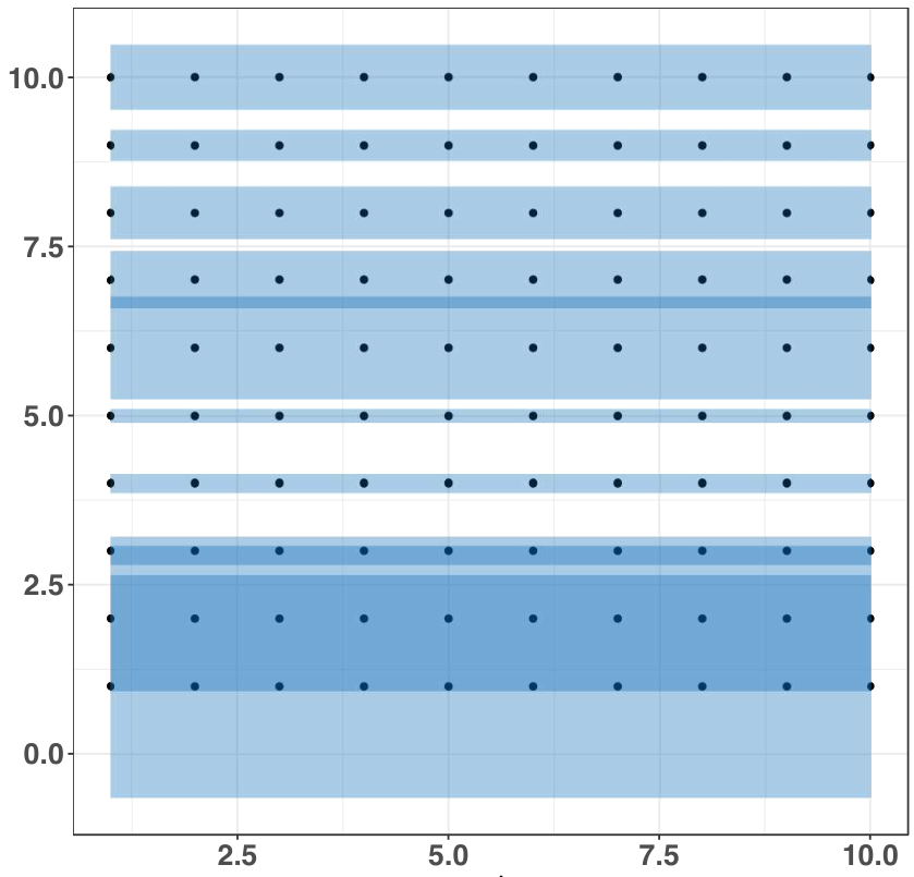
(b) 1st-order 
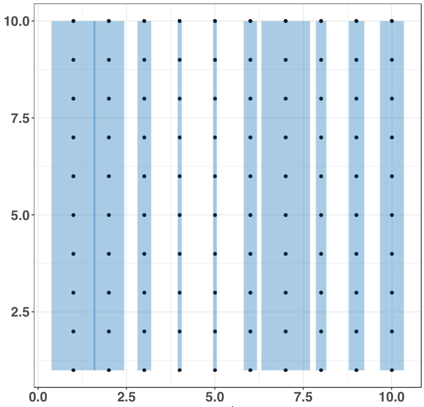
(c) 2nd-order Figure S1: The non-stationary additive covariance function in - with main effects and an interaction is the sum of the three terms: = + +. At each location the covariance function will make use the data contained within the shaded region in each of the plots. The 1st-order terms can pool together data across dimensions for long-range correlations, while the 2nd-order terms can capture local behavior in both dimensions. Appendix C Inference for one-dimensional problems
Algorithm 1 Metropolis-within-Gibbs (MWG) 1: , , , and2: for to do3: Draw:4: Compute:5: With probability set , otherwise set6: Run Adaptation for7: Draw:8: Set: † denotes matrix pseudoinverse. Use QR decomposition9: Draw:10: Set: and11: for to do12: Set:13: Compute:14: With probability set and ; otherwise set15: end for16: Run Adaptation for17: Draw:18: Compute:19: With probability set , otherwise set20: Run Adaptation for21: end forAlgorithm 2 Whitened Elliptical Slice Sampling (w-ELL-SS) 1: , , , , , and2: for to do3: Draw:4: Compute:5: With probability set , otherwise set6: Run Adaptation for7: Draw:8: Draw:9: Compute:10: Draw:11: Define:12: Propose:13: Update:14: Solve:15: if then16: Set:17: else18: if then19:20: else21:22: end if23: Draw:24: Go back to step 11.25: end if26: Draw:27: Compute:28: Solve:29: Compute:30: With probability set , and ; otherwise, set ,31: Run Adaptation for32: Draw:33: Set: † denotes the matrix pseudoinverse. Use QR decomposition34: Solve:35: end forAlgorithm 3 Marginal Elliptical Slice Sampling (m-ELL-SS) 1: , , , , and2: for to do3: Draw:4: Compute:5: With probability set , otherwise set6: Run Adaptation for7: Draw:8: Draw:9: Compute:10: Draw:11: Define:12: Propose:13: Compute:14: if then15: Set:16: else17: if then18:19: else20:21: end if22: Draw:23: Go back to step 11.24: end if25: Draw:26: Compute:27: Compute:28: With probability set , and ; otherwise, set ,29: Run Adaptation for30: end forAppendix D Inference for two-dimensional problems
Algorithm 4 Block Marginal Elliptical Slice Sampling (Block-m-ELL-SS) 1: , , , , , , , , , , , , and2: for to do3: Draw:4: Compute:5: With probability set , otherwise set6: Run Adaptation for7: Draw:8: Draw:9: Compute:10: Draw:11: Define:12: Propose:13: Compute:14: if then15: Set:16: else17: if then18:19: else20:21: end if22: Draw:23: Go back to step 13.24: end if25: Draw:26: Compute:27: Compute:28: With probability set and ,otherwise set29: Run Adaptation for30: Draw31: Repeat steps 6-29 for32: Draw:33: Draw:34: Compute:35: Draw:36: Define:37: Propose: is formed by stacking and38: Update: and39: if then40: Set: and41: else42: if then43:44: else45:46: end if47: Draw:48: Go back to step 36.49: end if50: Draw:51: Compute:52: Compute:53: With probability set , and ; otherwise, set .54: Run Adaptation for55: Repeat 49-53 for56: Draw57: end forAppendix E Experiments
(a) Experiment 1 (b) Experiment 2 (c) Experiment 3 Figure S2: One-dimensional simulated dataset. (a): 81 observations with domain and noise variance . (b): 350 observations with domain and noise variance . (c): 512 observations with domain and noise variance We consider three simulated datasets with different characteristics. The first example is a function which has smooth parts and edges, and it is also piecewise constant,
The second corresponds to a damped sine wave function,
The data was generated employing the Bumps function in Donoho and Johnstone (1995) and scaled to have zero mean and unit variance. Following Vannucci and Corradi (1999), we generate points in the interval [0,1] and use a signal-to-noise ratio equal to 5, such that the noise variance .
E.1 Experiment 1
MWG w-ELL-SS m-ELL-SS AR(1) 0.014 0.015 0.015 0.014 0.014 0.014 0.014 0.014 0.014 2.416 2.653 2.785 2.350 1.912 2.015 2.118 2.163 1.968 0.687 0.686 0.685 0.690 0.693 0.693 0.692 0.692 0.692 0.435 0.405 0.385 0.312 0.408 0.379 0.381 0.358 0.338 SE 0.031 0.043 0.055 0.013 0.013 0.015 0.013 0.013 0.013 0.678 1.183 1.165 1.888 2.147 1.709 2.119 2.142 2.145 0.690 0.698 0.674 0.692 0.692 0.691 0.692 0.693 0.693 0.543 0.545 0.539 0.188 0.191 0.476 0.186 0.181 0.174 Table S1: Experiment 1: Posterior mean estimates with both hyperpriors under various discretisation schemes () and three different algorithms. AR(1) SE Burned Non-burned Total time Burned Non-burned Total time MWG 0.01 16.78 16.80 28.02 NA 28.02 0.04 40.66 40.69 103.55 NA 103.55 0.10 76.84 76.94 265.16 NA 265.16 w-ELL-SS 0.04 14.55 14.58 0.18 24.84 25.02 0.30 51.90 52.20 0.82 103.05 103.86 0.70 127.67 128.37 3.22 249.15 252.37 m-ELL-SS 0.01 18.50 18.52 0.03 22.17 22.20 0.03 46.54 46.57 0.18 59.42 59.60 0.06 104.20 104.26 0.37 132.97 133.35 Table S2: Experiment 1: CPU time (minutes) for iterations. NA denotes that MWG for the SE hyperprior did not converge. Best values in boldface. MWG w-ELL-SS m-ELL-SS AR(1) 10452.5 7038.0 5070.5 5541.0 5313.1 4967.9 12234.4 11999.4 12124.1 5424.4 2150.5 1317.3 181.1 192.0 201.6 3146.7 3391.2 3282.9 22539.7 11131.5 6901.8 773.2 467.1 268.0 9337.0 3736.3 3557.9 25449.8 11648.3 7878.2 4635.0 5981.3 5264.1 30601.6 35096.7 47895.6 42146.1 27135.4 21528.7 8343.2 7485.8 8127.4 26530.5 27856.4 26881.2 1507.9 636.6 460.8 331.2 272.8 300.9 2068.6 2119.5 2243.5 SE 313.4 505.5 1986.6 6117.6 8008.2 2214.8 18983.7 15087.8 16750.4 2.1 7.5 6.7 214.0 195.7 289.1 3401.0 3498.8 3381.2 2.1 2.1 1.4 961.5 717.8 309.1 8434.1 7023.2 7391.8 91330.7 22391.1 117111.0 4992.2 5113.6 5989.6 28060.0 30737.0 28382.6 48.4 83.1 8678.6 11139.8 12676.2 2561.6 31456.3 33268.2 41623.7 16.6 77.4 82.3 57.5 29.5 3.6 367.8 246.9 293.3 Table S3: Results Experiment 1: ESS after burn-in period for both hyperpriors under various discretisation schemes () and employing three different sampling algorithms. Highest values in boldface. (a) , (b) , (c) , (d) , (e) , (f) , (g) , (h) , (i) , (j) , (k) , (l) , Figure S3: Experiment 1 with w-ELL-SS algorithm. (a)-(c): Estimated process with credible intervals for AR(1) hyperprior on different grids. (d)-(f): Estimated process with credible intervals for AR(1) hyperprior on different grids with observed data in red. (g)-(i): Estimated process with credible intervals for SE hyperprior on different grids. (j)-(l): Estimated process with credible intervals for SE hyperprior on different grids with observed data in red. (a) , (b) , (c) , (d) , (e) , (f) , (g) , (h) , (i) , (j) , (k) , (l) , Figure S4: Experiment 1 with m-ELL-SS algorithm. (a)-(c): Estimated process with credible intervals for AR(1) hyperprior on different grids. (d)-(f): Estimated process with credible intervals for AR(1) hyperprior on different grids with observed data in red.. (g)-(i): Estimated process with credible intervals for SE hyperprior on different grids. (j)-(l): Estimated process with credible intervals for SE hyperprior on different grids with observed data in red. E.2 Experiment 2
(a) , MWG with AR (b) , w-ELL-SS with AR (c) , m-ELL-SS with AR (d) , MWG with AR (e) , w-ELL-SS with AR (f) , m-ELL-SS with AR Figure S5: Experiment 2. Top row: estimated process with credible interval for AR(1) hyperprior with (a) MWG, (b) w-ELL-SS and (c) m-ELL-SS. Second row: estimated process with credible interval for AR(1) hyperprior with (d) MWG, (e) w-ELL-SS and (f) m-ELL-SS. AR(1) SE Burned Non-burned Total time Burned Non-burned Total time MWG 0.60 155.82 156.43 572.36 NA 572.36 w-ELL-SS 1.42 306.60 308.02 3.60 500.49 504.09 m-ELL-SS 0.25 308.67 308.92 1.17 330.04 331.22 Table S4: Experiment 2: CPU time (minutes) for iterations. NA denotes that MWG for SE hyperprior did not converge. Best values in boldface. MWG w-ELL-SS m-ELL-SS AR(1) 0.045 0.044 0.044 1.694 1.379 1.287 5.051 6.922 7.131 0.021 0.025 0.027 0.031 0.027 0.027 2.598 2.771 2.710 SE 0.072 0.044 0.044 0.594 0.965 .951 0.677 8.967 9.187 0.032 0.029 0.029 0.060 0.025 0.024 0.450 1.877 1.970 Table S5: Experiment 2: Posterior mean estimates obtained with both hyperpriors and employing three different sampling algorithms. Estimates are consistent across sampling algorithms, except for SE with MWG because the sampler did not reach convergence. MWG w-ELL-SS m-ELL-SS AR(1) 14505.3 17446.5 20673.4 116.3 282.6 2485.3 56.3 385.5 2421.7 7002.5 13637.9 37023.4 3424.5 8179.6 27585.5 92.6 145.7 1312.8 SE 444.5 18804.2 21169.3 5.0 1145.9 5996.4 7.4 919.4 3563.6 100000.0 37550.5 76574. 98891.7 14476.0 49195.2 44.8 91.0 668.4 Table S6: Experiment 2: ESS after burnin period for both hyperprior and employing three different sampling algorithms. Highest values in boldface. m-ELL-SS results in the highest efficiency scores. E.3 Experiment 3
MWG w-ELL-SS m-ELL-SS AR(1) 0.041 0.040 0.040 1.821 3.780 1.520 0.519 0.375 0.510 -0.519 -0.538 -0.535 2.097 2.110 2.086 0.033 0.029 0.033 SE 0.504 0.039 0.039 1.414 0.126 0.666 1.523 0.310 0.381 0.178 -0.499 -0.523 1.303 2.046 2.053 1.058 0.106 0.024 Table S7: Experiment 3: Posterior mean estimates obtained with both hyperpriors and employing three different sampling algorithms. MWG w-ELL-SS m-ELL-SS AR(1) 6975.6 3398.3 4638.5 489.5 8.2 155.1 1978.3 63.3 201.8 6875.2 3354.2 5220.6 4515.2 817.0 910.6 193.4 18.4 106.1 SE 2650.1 5072.4 12442.0 2.4 70. 153.7 2.5 310.3 1339.5 3522.7 49136.2 6397.9 2101.0 36809.1 4399.9 93.4 2.5 27.2 Table S8: Results for Experiment 3: ESS after burnin period for both hyperprior and employing three different sampling algorithms. Highest values in boldface. AR(1) SE Burned Non-burned Total time Burned Non-burned Total time MWG 32.48 297.78 330.27 1289.166 NA 1289.166 w-ELL-SS 106.43 592.95 699.38 6.02 1246.85 1252.87 m-ELL-SS 20.70 814.10 834.79 85.17 810.19 895.36 Table S9: Experiment 3: CPU time (minutes) for iterations. NA denotes that MWG for SE hyperprior did not converge. Best values in boldface. AR(1) SE Burned Non-burned Total time Burned Non-burned Total time MWG 27.86 249.14 277.00 956.78 NA 956.78 w-ELL-SS 45.91 258.61 304.52 402.77 NA 402.77 m-ELL-SS 9.39 375.90 385.29 42.98 397.12 440.10 Table S10: Computational time for Experiment 3 in a High Performance Computer. Algorithms were run for iterations. m-ELL-SS and w-ELL-SS speed up by a factor of approximately , while MWG by . E.3.1 Prior elicitation
As opposed to Experiment 1 and 2, where vague priors for covariance parameters sufficed, here we employ informative prior distributions for and . Knowledge about the parameters comes from the fact that the length-scales, for both stationary and non-stationary processes, are only identifiable between the minimum and maximum covariate distance. In this experiment, the maximum distance is 1 and the minimum is .0019; thus, the prior for each is inappropriate. Instead, we solve the system of equations in Section A to fix the hyperparameters. Indeed, arbitrarily fixing the hyperparameters can greatly affect the inferences. See for instance the estimated length-scale process with MWG and AR hyperprior in Figure S6, where we set the prior of to be a zero-centred GP with unit variance.
Figure S6: Posterior mean of lengh-scale for Experiment 3 with MGW and AR hyperprior with and . E.4 Two-dimensional synthetic data

(a) True 
(b) Posterior mean Figure S7: Results for two-dimensional simulated dataset. Appendix F Comparative Evaluation
(a) MAE= (b) MAE= (c) MAE= Figure S8: TGP model results for Experiment 1 with different chain lengths. (a): iterations with burn-in. (b): iterations with burn-in. (c): iterations with burn-in. (a) MAE= (b) MAE= (c) MAE= Figure S9: TGP model results for Experiment 2 with different chain lengths. (a): iterations with burn-in. (b): iterations with burn-in. (c): iterations with burn-in. (a) MAE= (b) MAE= (c) MAE= Figure S10: TGP model results for Experiment 3 with different chain lengths. (a): iterations with burn-in. (b): iterations with burn-in. (c): iterations with burn-in and thinning of . Increasing the number of iterations has a positive effect on the number of partitions found. However, without knowing the ground truth, it is hard to know beforehand if the algorithm has been run for long enough to find the appropriate number of partitions. 
(a) MAE= 
(b) MAE= 
(c) MAE= Figure S11: TGP model results for Experiment 4 (subset) with different chain lengths. (a): iterations with burn-in. (b): iterations with burn-in. (c): iterations with burn-in and thinning of . Appendix G Real data: NASA rocket booster vehicle
Figure S12: Results for NASA rocket booster vehicle experiment. Posterior mean of non-stationary interaction term. (a) (b) (c) (d) Figure S13: Posterior mean estimates of the stationary, one-dimensional length-scale processes with 95% credible intervals. (a): Length-scale process for . (b): Length-scale process for . (c)-(d): Length-scale processes for the interaction term, . Notice a dip at alpha=25 to recover the peak, and the small values of around mach=1.