Compiled August 24, 2026 \ociscodes010.1080 Adaptive Optics, 010.7350 Wavefront Sensing
Efficient, Nonlinear Phase Estimation with the Non-Modulated Pyramid Wavefront Sensor
Abstract
The sensitivity of the the pyramid wavefront sensor (PyWFS) has made it a popular choice for astronomical adaptive optics (AAO) systems. The PyWFS is at its most sensitive when it is used without modulation of the input beam. In non-modulated mode, the device is highly nonlinear. Hence, all PyWFS implementations on current AAO systems employ modulation to make the device more linear. The upcoming era of 30-m class telescopes and the demand for ultra-precise wavefront control stemming from science objectives that include direct imaging of exoplanets make using the PyWFS without modulation desirable. This article argues that nonlinear estimation based on Newton’s method for nonlinear optimization can be useful for mitigating the effects of nonlinearity in the non-modulated PyWFS. The proposed approach requires all optical modeling to be pre-computed, which has the advantage of avoiding real-time simulations of beam propagation. Further, the required real-time calculations are amenable to massively parallel computation. Numerical experiments simulate a PyWFS with faces sloped 3.7∘ to the horizontal, operating at a wavelength of 0.85 m, and with an index of refraction of 1.45. A singular value analysis shows that the common practice of calculating two "slope" images from the four PyWFS pupil images discards critical information and is unsuitable for the non-modulated PyWFS simulated here. Instead, this article advocates estimators that use the raw pixel values not only from the four geometrical images of the pupil, but from surrounding pixels as well. The simulations indicate that nonlinear estimation can be effective when the Strehl ratio of the input beam is greater than 0.3, and the improvement relative to linear estimation tends to increase at larger Strehl ratios. At Strehl ratios less than about 0.5, the performances of both the nonlinear and linear estimators are relatively insensitive to noise, since they are dominated by nonlinearity error.
1 Introduction
The concept of creating a wavefront sensor for adaptive optics (AO) by focusing a telescope beam onto the vertex of a glass pyramid and then re-imaging the pupil with the light exiting the bottom of the pyramid is due to Ragazzoni.[1] This has come to be known as the pyramid wavefront sensor (PyWFS), and its design is shown schematically in Fig. 1. In the standard configuration, the beam passes through a four-sided pyramid, and then a relay lens re-images the pupil, creating four images that carry information about the wavefront. Usually, the pyramid is a square pyramid, but other configurations have been considered.[2, 3, 4, 5] The desirability of the PyWFS is due to the fact that it is much more sensitive (in terms of performance for a given guide-star magnitude) than the Shack-Hartmann array for low-order modes, and for high-order modes, it is equally sensitive.[6, 7, 8, 9]
The PyWFS’ current status as the most promising and powerful type of wavefront sensor for AO was achieved with release of the unprecedented results produced by the First Light AO system on the Large Binocular Telescope, which routinely delivers Strehl ratios greater than 0.8 in the H-band.[10, 11] The PyWFS has become the wavefront sensor of choice in much of the AO community, and is currently employed by MagAO, SCExAO, and the First Light Adaptive Optics (FLAO) system, among others.[12, 13, 11] Development of PyWFS technology continues to be high priority research, as the European Extremely Large Telescope (E-ELT), the Giant Magellan Telescope (GMT) and the Thirty Meter Telescope (TMT), all members of the coming generation of 30-meter class telescopes, plan to utilize the PyWFS for their AO programs.[14, 15, 16]

A necessary consequence of the high sensitivity of the PyWFS is nonlinearity, meaning the intensity seen by the PyWFS detector is nonlinear in the phase of the wavefront. In order to reduce the nonlinearity, all current implementations of the PyWFS use dynamic modulation of the input beam, in which the focal point is steered around the tip of the pyramid with a period at least several times shorter than the exposure time.[1] This practice indeed improves the linearity range of the device, but at the expense of sensitivity.[18, 19] In the context of multi-conjugate AO, Ref. [20] proposes the Very Linear Wavefront Sensor, which operates on a locally closed loop to bring the signal into the linear regime. Ref. [21] proposes treating nonlinearity by measuring the nonlinear response to various wavefront modes deliberately imposed on the beam via DM commands. This scheme cannot treat the fact that the nonlinear response will depend on the instantaneous shape of the wavefront and this effect must be negligible for it to be successful. We note that several groups have proposed using spatial light modulators in lieu of mechanical beam steering.[22, 23]
The loss in sensitivity caused by the modulation may not be acceptable for the needs of so-called "extreme AO" (ExAO).[24] That is why several groups, including the GMT team, hope to use the PyWFS without modulation, using a scheme in which the control loop is first closed while employing modulation, and then the modulation would be turned off.[25] In these applications, it is likely that the PyWFS will receive a beam that has been partially corrected by atmospheric distortion by a first-stage AO system. The two-stage AO scheme is currently employed by several extreme AO systems including SCExAO, which takes the beam after it has passed through the Subaru telescope’s AO188 system.[13] This article argues that nonlinear estimation of the phase of the wavefront measured by the non-modulated PyWFS has the potential to be a useful component of such a scheme for ExAO, and that it is worthy of more detailed study.
The PyWFS is intractable analytically, and analytical results have relied on various simplifications and assumptions, including treating the pyramid faces as Foucault knife-edges and neglecting interference between the pupil images [e.g., 18, 17, 8]. Perhaps as a result of such studies, the PyWFS is often considered to be essentially a slope-sensor that can be treated as a Shack-Hartmann array, once the sum of one pair of images has been subtracted from the sum of the other pair.[17] Later literature has discussed the fact that PyWFS is not simply a slope sensor.[2, 4]
The first attempt (that we know of) to treat the nonlinearity in the PyWFS computationally was published by Korkiakoski et al.[26] That paper is similar to the one here in that a forward model of the PyWFS based on Fourier optics is used to find a relationship between the measurements and the unknown phases, but it neglects interference between the beams exiting the pyramid; this interference effect is not negligible for the simulations presented below. The nonlinear estimation method in that article utilizes only the gradients of the PyWFS intensities, whereas one of the algorithms in this article utilizes a more powerful nonlinear solution method enabled by calculation of the Hessians of the intensities. Crucially, the paper by Korkiakoski et al. does not show how the gradient computations can be dramatically accelerated by pre-computation of the modeling calculations and efficient representation of the field in the pupil plane, as is done here.
Ref. [27] provides a comprehensive review of reconstruction methods for the PyWFS and it also introduces two new reconstruction algorithms. The standard method for reconstruction is called matrix-vector multiplication, in which one pre-computes the (possibly regularized) inverse of a matrix that maps the deformable mirror (DM) commands to the intensity changes. All of the current reconstruction methods use a linear relationship between the sought-after quantities (i.e., phases or deformable mirror commands) and the intensity measurements. Almost all (closed-loop) implementations of the PyWFS employ a scheme in which the DM and PyWFS are calibrated only in reference to each other, i.e., the calibration measurements use intensity changes seen by the PyWFS detector in response to known DM commands. In contrast, the methods described here are enabled by a pre-computed and independently calibrated model of the PyWFS. One advantage of using such a pre-computed model is that no propagation computations are performed in real time, allowing time-consuming numerical methods for optical modeling to be employed. Specifically, we will show that the gradients and/or Hessians required by standard methods for nonlinear optimization can be implemented efficiently in a massively parallel fashion, making deployment on real-time AO control systems a realistic possibility.
2 Fourier Optics Model
One crucial feature of the wavefront estimation method presented here is that it can work with any numerical model used to simulate the pyramid wavefront sensor, with no consequences for the amount of real-time computation required. Indeed, the validity of the estimation method relies only on the linear relationship between the electric field at the detector and the electric field in the pupil plane, and this linearity will hold for any wavefront sensor so-far ever considered for AO. (Nonlinear devices, such as optical parametric amplifiers, would violate the linearity assumption.) The numerical model employed here for the purpose of algorithm development is based on Fourier optics.[28] In these simulations, the lenses are treated as thin phase-screens that act mathematically as Fourier transform operators. The required transforms are implemented numerically with discrete Fourier transforms (via an FFT algorithm). A Fourier optics treatment of the PyWFS was first published in Ref. [26] and was later placed into a generalized framework in Refs. [19, 4]. A sophisticated ray-tracing tool for the PyWFS was presented in Ref. [29].
 |
 |
Consider quasi-monochromatic light at wavelength (wavenumber ) impinging on the PyWFS entrance pupil , and let the electric field in that pupil be represented by where is the two-dimensional (2D) spatial coordinate. This complex-valued field can be written in terms of its real-valued amplitude and real-valued phase as . In a PyWFS, the entrance pupil light is brought to a focus with a lens of focal length , and the field in the focal plane , apart from an inconsequential phase factor and a multiplicative constant, is given by [28]:
| (1) |
The slope of the pyramid faces imparts a spatially variant phase shift to the field in the focal plane. Let us call this effect the phase ramp, denoted as , where is the face index [so, for a square pyramid ], and it is given by
| (2) |
where is the index of refraction of the pyramid glass, and is the height of the th pyramid face relative to the horizontal. After the phase ramp is applied, the light propagates through the rest of the pyramid, exits the prism’s bottom, and then encounters the collimator lens. The collimator lens re-images the pupil, but now there is one image of the pupil corresponding to each face of the pyramid (assuming the slope of the pyramid is great enough to separate them; see Ref. [3] for a counter-example). The collimator lens essentially takes a second Fourier transform of the light, and the field on the detector is given by:
| (3) |
where is the 2D spatial coordinate in the detector plane, (without the index subscript) is the collection of all of the pyramid faces, and the focal length of the collimator lens is also taken to be . The spatial limits of integration are taken to be infinite (since the field in the focal plane is essentially contained within any physical boundary of the apparatus). Combining Eqs. (1) and (3) gives an expression for the pyramid operator :
| (4) |
Note that the pyramid operator is linear in , a fact that will prove critical in designing efficient estimation algorithms. Eq. (4) shows that the pyramid operator essentially takes two Fourier transforms of the pupil field (applying the phase ramp in between), thereby creating inverted images of the pupil. Then, the field impinging on the detector is conveniently re-expressed as:
| (5) |
The intensity of the light on the detector surface is:
| (6) |
where the superscript ∗ signifies complex conjugation. The goal of wavefront sensing is, of course, to obtain information about the pupil field from the measurements of the intensity . The sought-after information is usually the phase , but the device is also sensitive to the amplitude , which also can be estimated under favorable conditions.
3 Discretization of the Model
Any numerical model must relate the pupil field at a discrete set of points , to the detector field at another discrete set of points , , where and are the sets of all such points in the model and and are the numbers of points in each set. Thus, the detector field at the point , , can be considered to be a function of the pupil field at each point in the set , and, using the pyramid operator Eq. (4), this can be expressed as:
| (7) |
where the pyramid operator has been taken to have a discrete implementation via some numerical model. It is useful to define a basis set on the points in the pupil . The basis vectors , are defined as:
| (8) |
where only the th of entries is nonzero. Then, via the linearity property of the pyramid operator, Eq. (7) can be written in terms of the basis vectors as:
| (9) |
Eq. (9) shows that once the pyramid operator has been evaluated for each of the basis vectors , the detector field can be calculated with very few operations, independently of the complexity of the optical model used to calculate the pyramid operator. Indeed, can be stored as a matrix, and then Eq. (9) can be carried out with a single (complex-valued) matrix-vector multiplication for any desired entrance pupil field represented as . For the purposes of discussing the algorithms in the remainder of this article, it will be assumed that the values of have been stored and therefore require no computation.
3.1 Pupil Field Representations
We have not specified how the pupil field will itself be represented, and below we present several options. Each representation expresses the set of field values in terms of real-valued parameters . The first option is called the "PolarPixel" representation:
| (10) |
in which through represent the phases of the pupil field at each point in the set and through represent the amplitudes, so the number of parameters is twice the number of pupil plane pixels, i.e., . If the amplitude of the field is known (or perhaps measured by a scintillation monitor), or amplitude effects are ignored, then Eq. (10) can be simplified to produce the "PhasePixel" representation:
| (11) |
where the (positive, real-valued) amplitudes are assumed to be known. If amplitude effects are ignored, then the can be set to the expected value of the magnitude of the pupil field, which can be estimated by summing up all of the counts on the detector to get a mean modulus of the pupil field and applying the appropriate calibrations. In the PhasePixel representation (so, there is one parameter for each pupil plane pixel). Another representation with similar efficiency advantages (to be described later) is called the "ReImPixel" representation, in which one models the real and imaginary parts of the field directly:
| (12) |
where the number of parameters is twice the number of pupil plane pixels, i.e., . Thus, in the ReImPixel representation, the amplitude of the pupil plane field at point is given by and its phase is given by .
In contrast to the pixel basis functions above, consider a modal representation of the phase (ignoring amplitude effects for simplicity), called "ModalPhase." In the ModalPhase representation, the phase is taken to be a linear combination of modal functions , such as Zernike polynomials, and the pupil plane field is given by:
| (13) |
where the amplitudes are taken to be known as in the PhasePixel representation. Below, we will see that the ModalPhase representation carries a significant computational cost burden that the other representations described above do not share.
3.2 Detector Intensity and its Derivatives
The estimation algorithms will require expressions for the derivatives of the intensity in the detector plane with respect to the parameters . The first step in calculating the intensity derivatives is to calculate the "field Jacobian," which is the derivative with respect to the parameters of the complex-valued electric field in the detector plane. Unless otherwise stated, all formulae given in the remainder of this article assume the PhasePixel representation, but corresponding expressions for the other representations can be derived similarly. The field and the field Jacobian are given by Eqs. (9) and (11), resulting in:
| (14) | |||||
| (15) |
Thus, the field Jacobian can be calculated with only several times floating-point operations (FLOPs), where the reader will recall that for the PhasePixel representation and the are taken to be known amplitudes. The most efficient way to calculate the field values in Eq. (14) is to calculate the field Jacobian from Eq. (15) first. Then, for each position , sum the corresponding values of the gradient (multiplied by ). Since elements of the field Jacobian can be calculated completely independently from each other, this can be implemented in parallel. The field Hessian, i.e., the second derivative matrix of the field at a given point in the detector plane , has a convenient property that follows directly from Eq. (15):
| (16) |
In order to appreciate the computational simplicity of the PhasePixel representation compared to the ModalPhase representation, consider the expressions equivalent to Eqs. (14) and (15) under the ModalPhase representation:
| (17) | ||||
| (18) |
In particular, one should note the double summation in (18), as opposed to no summations in (15). Unlike the PhasePixel representation [see (16)], the off-diagonal elements of the field Hessian under the ModalPhase representation are non-zero, and their cumbersome formula is not given here.
Next, we derive expressions for the derivatives of the intensity in the detector plane with respect to the unknown parameters under the PhasePixel representation. The intensity at the detector is given by , and the intensity Jacobian is calculated easily with the help of Eq. (15):
| (19) |
where "c.c." indicates the complex conjugate of all preceding terms. Note that for any quantity , , where is the real part of [the imaginary part of is denoted by ]. This shows that calculating the intensity Jacobian requires little more computation, once the field Jacobian has been calculated from Eq. (15). The Hessian matrix of the intensity at the point is given by differentiating Eq. (19) with the help of Eqs. (14) through (16):
| (20) | ||||
| (21) |
Note that the intensity Hessian in Eqs. (20) and (21) is calculated with little more effort, given the already determined values of the field Jacobian in Eq. (15). Each of the detector plane positions has a Hessian matrix associated with it, each of which has unique elements (due to symmetry), for a total of elements needed to specify the Hessian at every position in the detector plane. According to Eq. (20), each of these quantities can be calculated with only a few FLOPs, and it is clear that this task can be achieved in a massively parallel manner, since the computation of these elements can be performed independently. It is worth remarking that much more computation would be required to calculate the Hessian in the ModalPhase representation for a comparable value of , as can be seen by Eq. (17) and considering the steps needed to derive the equations corresponding to Eqs. (19) through (21). In contrast, the PolarPixel and ReImPixel representations have (instead of ), but otherwise have similar computational complexity to the PhasePixel representation.
3.3 Effective Sparsity of the Hessian Matrices
Nonlinear estimation based on Newton’s method for optimization requires the Hessian of the cost function, which will require calculations of the Hessians of the intensities at the individual detector pixels. Calculating the Hessian matrix for each of the locations on the detector requires determining quantities. Even though the matrix elements in Eqs. (20) and (21) can be calculated with only a few FLOPs (once the field Jacobian has been calculated), nevertheless, this could be a daunting task under real-time constraints. Approximation of the Hessian of the intensity at a given pixel by a sparse matrix may be a useful strategy to speed real-time computation.
The sparsity pattern will depend on the pixel index , but it can be pre-computed, since the particular values of the parameters only serve to rotate the field Jacobian values in the complex plane [see Eqs. (15) and (20)]. In order to gain a first look at the effective sparsity of one of these Hessian matrices, we used the PyWFS simulations described later to examine the Hessian matrix associated with the intensity at the central pixel in the upper-left pupil image (see Fig. 2). Let us denote that pixel with the index . The sparsity was evaluated on the matrix , which is the absolute value of each matrix element averaged over 100 random realizations of the parameters . In each of the 100 random realizations, all of the values of were given (independent) random values between and . If represents the largest entry in , we found that about of the matrix elements are greater than and of them are greater than .
Determining the utility of sparse approximations to these Hessians is beyond the scope of this article, as it must be done within the context of a detailed study of massively parallel implementations of the various estimation algorithms on a real-time system. We only mention it because it may be useful in the future.
| item | size | |||
|---|---|---|---|---|
| p | p | p | ||
| 0 | ||||
| 0 | ||||
| 0 | 0 | |||
| 0 | 0 | |||
| 0 | 0 |
4 Estimation Procedures
The goal of the inference procedure is to estimate the parameters from the intensity measurements. The intensity values measured by the detector are noisy versions of the true intensities and can be modeled as:
| (22) |
where is the detector pixel index, are the measured intensity values and represents the (unknown) contribution of noise to the measurement, e.g., from photon counting (shot) noise and detector readout noise. It will be assumed that the are samples from zero-mean random process so that , where is the expectation operator.
In this section, two estimation paradigms will be considered, linear least-squares and nonlinear least-squares. Linear least-squares is representative of control algorithms that use a linear response matrix to estimate the wavefront. Nonlinear least-squares can be more accurate than linear least-squares because the model is nonlinear in .
4.1 Preprocessing and Amplification of Nonlinearity Error
4.1.1 Preprocessing Options
There are a number of options for pre-preprocessing the measured intensities before applying an estimation algorithm. After this choice has been made, one can generate the vector of preprocessed measurements , where is used as input into a regression scheme. Let be the number of detector pixels within a single pupil image, so that geometrical optics would predict a total of illuminated pixels. Here, we will cover four preprocessing choices. Two of these choices are slope preprocessing, which is common in the PyWFS community, and two are non-slope preprocessing. Each preprocessing option is given a name:
- 1.
"FourImages" is simply the raw intensity values of the pixels within the four geometrical images of the pupil. It is an example of non-slope preprocessing. In this case, the vector has components.
- 2.
"AllPixels" is the raw intensity values of all of the pixels on the detector, whether or not they are within one of the four geometrical images of the pupil, and it is also non-slope preprocessing. In this case, has components where is the total number of detector pixels.
- 3.
"NomalizedSlope" is the most common in the AO community, in which the 4 pupil images are reduced to two "slope" images.[18] These images are produced by adding and subtracting pairs of images, and dividing by the mean image. This results in a having components.
- 4.
"UnnormalizedSlope" is the same NormalizedSlope, except there is no division by the mean of the four pupil images. Here, also has components.
Thus, with FourImages and AllPixels, the components of have a very simple relationship to the values of detector intensities in (22), namely,
| (23) |
Under the UnnormalizedSlope preprocessing, represents two slope images, so can be split into a vertical slope image and a horizontal slope image , in which the elements are given by:
| (24) |
where is the intensity measured in the th pixel in the upper-right pupil image, and , , are the corresponding values in the upper-left, lower-left and lower-right pupil images, respectively. NormalizedSlope preprocessing is similar, except that the horizontal slopes are divided by the mean of the four pupil images, so:
| (25) |
Note that if the noise in the values is modeled by a zero-mean random process as in (22), then the division in (25) implies that NormalizedSlope values will have noise statistics that are not given by a zero-mean random process, whereas the other three representations have noise statistics that are straightforward (given the processes ).
One fact that should be appreciated is that a signficant fraction of the light can fall outside of the 4 four geometrical pupil images. The amount of light lost by only collecting the light within the four geometrical pupil images increases with Strehl ratio. This effect is shown in Fig. 3 for the simulation experiments described in detail later. The figure shows that when the Strehl ratio is 0.1 only about 10% of the light is lost, but that fraction increases to about 56% at a Strehl ratio of 1.0.


 |
 |
4.1.2 Information Loss in Slope Sensing
Besides discarding some of the light, as shown in Fig. 3, there is a more subtle, yet far more detrimental problem associated with slope sensing with the non-modulated PyWFS. This is the error caused by amplification of the nonlinearity by the inversion used to obtain the phases. Developing these arguments will require a bit of detailed treatment of the error incurred by first order Taylor expansions (nonlinearity error) and its consequences for linear regression. Consider the following generic nonlinear regression model:
| (26) |
where has components (the number measurements), is a vector of unknown values with components that we wish to determine, is a vector of nonlinear functions of , and is a vector of zero-mean random processes representing noise. Sometimes is called the measurement function, since it relates to the measured values. The use of , , and is consistent with our previous uses of these symbols above, but for this section, they are intended only to describe the generic nonlinear regression model shown in (26). The Taylor expansion of about the point can be written in terms of ’s Jacobian matrix , so that the measurement function can be rewritten as:
| (27) |
where is the Jacobian matrix, and the new vector of functions (with components) accounts for the error incurred by the linearization, such that . The vector of functions will be called the "nonlinearity error." To economize, let us make the following change in notation: , . Then (26) becomes:
| (28) |
If we ignore the nonlinearity error , which is necessary for linear regression, it can be shown that the least-squares estimate of minimum norm is provided by the pseudo-inverse of the matrix , written as , via the equation:
| (29) |
In order find , first perform the singular value decomposition (SVD) of as (the superscript T indicates matrix transposition), where and are unitary matrices and is a diagonal matrix of singular values . The set of singular values , ordered from largest to smallest, is also known as the spectrum of the matrix or the spectrum of singular values. Then , where is a diagonal matrix of the inverses of all of the non-zero singular values, i.e., . Where the singular values are zero (or deemed to be numerically small) the corresponding entries in the diagonal of are assigned values of zero.[30]
In order appreciate how the inversion in (29) can amplify the noise and the nonlinearity error , substitute (28) into (29):
| (30) |
where the unitary property of (i.e., , where is the identity matrix) has been utilized. The matrix is a diagonal matrix with values of unity where and 0 where (or small enough numerically to be considered zero). In the first term of (30), the components of receive no amplification since is unitary. It is easy to show that . Further, if all of the singular values are greater than zero (i.e., ), then . On the other hand, the small singular values in in the second term of (30) will amplify both the nonlinearity error and the noise . Thus, small singular values are detrimental to the accuracy of the inversion even in the case in which there is no noise (i.e., ). One popular method of mitigating this noise amplification, called SVD truncation, is to replace with 0 on the diagonal of whenever is below some threshold. When the SVD is truncated, the associated modes are forced to 0. [The modes under discussion here are singular vectors (i.e., the columns of the matrix ), not the functions in (13).]
NormalizedSlope, UnnormalizedSlope, FourImages and AllPixels (see Sec. 44.1.1) each correspond to a different version of the measurement function , according to Eqs. (23) through (25), each of which relates to the computational model of the detector intensity via (22). Then, the calculation of the Jacobian matrix for each preprocessing option can be calculated using (19). Fig. 4 shows the resulting singular values of , where it can be seen that the singular values obtained using slope preprocessing (NormalizedSlope and UnnormalizedSlope) decline more steeply than they do for non-slope preprocessing (FourImages and AllPixels). For each case (NormalizedSlope, UnnormalizedSlope, FourImages and AllPixels), the relevant Jacobian was evaluated for a flat wavefront, i.e., , and the singular values were calculated with a standard SVD algorithm. Each curve in Fig. 4 is normalized by its first singular value, which is the largest one. In all cases, the final singular value is 0, corresponding to the piston term, which cannot be determined from a WFS. (The simulations showed that the final column of the matrix is a vector in which all values are the same, confirming that the final singular value does indeed correspond to the piston term.)
The more rapid decline in singular values for the slope preprocessing has dramatic consequences for estimation of the wavefront. Fig. 5 shows RMS phase error obtained by applying the pseudo-inverse formula [(29)], as a function of the input Strehl ratio of the input beam. Each data point in Fig. 5 is a result of 60 trials in which the 797 phase values were sampled independently from a normal distribution with a standard deviation given by by (Ruze formula), where is the Strehl ratio of the input beam. The error bars (at least those large enough to be visible) indicate the standard deviation of the RMS error over the 60 trials. The piston term (i.e., the mean) of these randomly generated phase values was subtracted in each trial, so no error was caused by the final zero on the diagonal of , which forces the piston term of the estimate to be zero. All of the trials used to create this figure had no noise, so . Therefore, all of the errors in the estimates shown in the figure were caused by the nonlinearity error . The figure shows that the inversions corresponding to FourImages and AllPixels far outperform the inversions corresponding to NormalizedSlope and UnnormalizedSlope, with UnnormalizedSlope being the slightly better of the two.
The black curve labeled "no gain" in Fig. 5 corresponds to an RMS error equal to . Whenever an estimator is below this curve it is providing some information about the wavefront, but when an estimator is above this curve, it is performing more poorly than simply using as the estimator. The figure shows that NormalizedSlope and UnnormalizedSlope only provide gain for Strehl ratios greater than about 0.9, and actually provide negative gain for lower Strehl ratios. In contrast, the estimators corresponding to FourImages and AllPixels provide gain for all Strehl ratios in the figure, down to a Strehl ratio of about 0.1. In order for the slope preprocessing to provide gain at lower Strehl ratios, it would be necessary to either apply SVD truncation as explained above, and/or use a ModalPhase representation with a number of modes that is small enough to avoid problematic singular values. Both of these approaches effectively trade numerical stability for decreasing the spatial resolution of the estimated wavefront.
Thus, this analysis indicates that the traditional slope preprocessing is likely to prove suboptimal for the non-modulated PyWFS and it will not be considered further in the remainder of this article. In addition, from this point forward, we will only consider the AllPixels preprocessing option, since the FourImages discards some of the light at high Strehl ratio, as Fig. 3 shows.
4.2 Linearized Least-Squares with Regularization
The pseudo-inverse was introduced above in order to show how inversion can amplify noise and error due to nonlinearity. While one could perform least-squares estimation from noisy data by employing a truncated pseudo-inverse, this method does not generalize to nonlinear estimation. Instead, here we introduce a regularization term that mitigates the effects of small singular values in the Jacobian matrix. The same term can be included in nonlinear estimation procedures, as we demonstrate later.
Going forward under the AllPixels preprocessing for the reasons given above, the vector of intensity measurements has components defined by Eqs. (22) and (23). It will economize the notation to redefine and via: , , where is all values of arranged into a column vector. The unknown parameters are related to the measurements via (28). Here, the symbols are defined specifically for the PyWFS estimation problem, not in generic terms as they were when (28) was first presented. The linearized model can be expressed in terms of the Jacobian matrix :
| (31) |
which is the Jacobian evaluated at . In practice, would correspond to a flat wavefront (zero phase) or take into account known static aberration. The Jacobian can be calculated from Eq. (19) for the PhasePixel representation.The linearized least-squares solution is a minimizer of the (scalar) cost function:
| (32) |
where is a matrix of the measurement weights ( is diagonal for uncorrelated noise), is a regularization matrix and () is a regularization parameter that controls the strength of the regularization. Taking the measurement weight to be the inverse of the measurement noise covariance matrix corresponds to the maximum-likelihood cost function for Gaussian noise statistics. The minimizer of Eq. (32) is easily shown to be:
| (33) |
Then, the linear least-squares estimate is . A proper choice of and non-zero choice of ensures invertibility of the matrix in Eq. (32); also see comments in Ref. [26]. Once the quantities , , and have been chosen, the matrix can be pre-computed, so that calculating the linear least-squares estimate only involves a single matrix-vector multiplication.
Common choices for include the identity matrix and finite differencing operators implemented with values of (where means "of order unity") on the appropriate diagonals. For example, if is one such matrix, then . Matrices of this type have a largest singular value on the order of unity, so that a baseline value for can be calculated by where is the vector of synthetic intensity values associated with a flat wavefront (i.e., in the PhasePixel representation). Then, would correspond to a solution dominated by regularization, and we would expect optimal values of to correspond to , where .
4.3 Nonlinear Least-Squares
The purpose of the nonlinear least-squares is to account for the fact that the measurement function is nonlinear in the parameters . The nonlinear cost function corresponding to Eq. (32) is:
| (34) |
(34) does not have defined with subtracted, nor is defined with subtracted, as they were in (32), since (34) is not a linearization. The discussion below will require the gradient and Hessian of the cost function:
| (35) | ||||
| (36) |
where is the th element on the diagonal of and is an element of the regularization matrix . Note that (35) and (36) assume that the weight matrix is diagonal. The needed derivatives of the intensity are shown in Eqs. (19) through (21) for the PhasePixel representation. Since each element of the Hessian of the cost function requires a sum over pixels, calculation of this Hessian requires the determination of quantities. While the Hessian of the cost function is not itself sparse, the intensity Hessians in the second term of Eq. (36) may have useful sparse approximations, as already discussed in Sec. 33.3.
(34) represents an unconstrained nonlinear optimization problem, in which one attempts to find the value of the parameter vector that minimizes . Unconstrained nonlinear optimization has two goals that often oppose each other: finding a minimum with minimal computational cost and avoiding local minima. In some optimization problems (e.g., nonsingular quadratic cost functions), there is only one local minimum that is the global minimum. Otherwise, avoiding local minima requires global minimization methods, such as simulated annealing, that involve stochastic searching of the parameter space. These methods are very slow and are not suited for the needs of control systems or large batch estimation. Local optimization methods, on the other hand, do not attempt to find a global minimum. Instead they find the local minimum corresponding to the initial guess; one could say "they just go down the hill" [31]. As nonlinear optimization is always iterative, it requires an initial guess. One choice for this guess is the linear least-squares solution , given above, and that is what has been used for the numerical examples shown later.
In terms of iteration counts, the most efficient local optimization method is often Newton’s method, and it almost always converges in many fewer iterations than gradient descent. This is because Newton’s method is based on successively approximating the cost function with quadratic functions, as opposed to gradient descent, which does not account for the local curvature of the cost function. Newton’s method requires the gradient and Hessian of the cost function, shown here in Eqs. (35) and (36) for the PhasePixel representation. In its purest form, the Hessian matrix needs to be inverted, but in practice this is avoided by solving a system of equations iteratively with the conjugate gradient algorithm. Thus, the cost of a single Newton iteration is often dominated by calculating the Hessian and performing the multiple iterations of the conjugate gradient algorithm. Calculating the Hessian matrix is sometimes prohibitive and this has given rise to a variety of "quasi-Newton" methods that only require the gradient of the cost function, avoiding explicit calculation of the Hessian. One widely popular quasi-Newton method is the Broyden–Fletcher–Goldfarb–Shanno (BFGS) algorithm, and that is the algorithm we discuss here and implement in the simulation experiments below. The BFGS algorithm updates an approximation to the inverse of the Hessian of the cost function with every iteration, so it almost always takes multiple BFGS iterations to achieve the minimization attained by a single Newton iteration. The cost of a single BFGS iteration has three primary contributors: a line search requiring multiple function and gradient evaluations, and a matrix-matrix multiplication required to update the approximation to the inverse Hessian.[31] Whether an implementation of Newton’s method or a quasi-Newton method would be more efficient for real-time nonlinear estimation for a PyWFS depends on the details of how the parallelization is implemented and how much sparsity can reduce the cost of calculating an approximate Hessian (see Sec. 33.3). A detailed comparison of Newton and quasi-Newton methods for nonlinear PyWFS estimation under different parallelization schemes is beyond the scope of this article. Instead, this article argues that the nonlinear cost function, its gradient and its Hessian can be implemented efficiently and in parallel, thus enabling, in principle, both Newton and quasi-Newton methods.
4.4 Enforcing Zero-Mean Phase
The WFS has no response to the piston term, causing a zero singular value in the Jacobian matrix of the measurement function (see Fig. 4). Depending which representation of the wavefront is being used, there are several ways to force the piston term to be zero and resolve the issue of the zero singular value. If one is using ModalPhase, simply remove the piston term from the expansion in (13). In this way, the singular value of 0 never arises. This approach assumes the remaining modes have no piston component. In the PhasePixel representation when using linearized least-squares, augmenting the Jacobian with a row of and appending with 0 (a weight value, , should also be appended to the diagonal of ) explicitly forces the mean of the estimated phases to be 0. This makes the singular value corresponding to the piston term finite. When using nonlinear least-squares with the PhasePixel representation, adding a another term, (where is a weight), to the cost function in Eq. (34) achieves the same end. In practice, the weight value should be large enough that the mean phase is quite close to zero in the final solution, but not large enough to cause numerical difficulties due to finite floating-point precision.
4.5 Application to Time-Series
So far, we only addressed the problem of estimating a single wavefront, not a time-series of wavefronts. The problems should be treated differently since the wavefront at is highly correlated with the wavefront at time , where is the time-step of the AO loop, typically on the order of 1 ms. Thus, an optimal estimation method would take advantage of this information. The typical solution in linear estimation is Kalman filtering, and there are standard extensions to treat nonlinearities. Kalman filtering can become computationally expensive due a certain matrix inversion, and there is a large literature devoted to dealing with this difficulty.[32] One way to account for the temporal correlation in the wavefront within the framework already presented is to add the following term to the cost function when calculating the solution for :
| (37) |
where is the estimate from the previous time-step, is a weight, and is an matrix. Note that if is taken to be the identity matrix, then the penalty term in (37) has a form that is similar to the regularization penalty in Eqs. (32) and (34), and it can be used to mitigate the effects of singularity or near-singularity in the intensity Jacobian [(19)].
Another important aspect of applying the linear and nonlinear least-squares algorithms to time-series concerns the choice of the starting guess. The estimate at the previous time-step, , is an obvious choice; another choice would be , where in order to improve stability.
5 Simulation Experiments
A numerical simulation of the PyWFS with geometrical parameters similar to the PyWFS on the SCExAO/Subaru generated the results shown in this article.[13] The prism is taken to be a square pyramid with each face making an angle to the horizontal of and an index of refraction of 1.452 at the operating wavelength of m. The telescope optics reduce the m diameter beam down to a diameter of mm, and a lens with focal length focuses the beam onto the tip of the pyramid.
Numerically, the beam in the entrance pupil was sampled with 33 pixels across, resulting in 797 pixels in the circular pupil (no "spiders" or other obscurations were included). In order to simulate a wavefront under the PhasePixel representation, each of the entrance pupil pixels had a phase (thereby creating the vector) assigned. The 797 amplitude values, i.e., in (11), were taken to be unity. We did not consider scintillation effects. In order to perform the Fourier transforms in Eq. (4), these 797 pixels (forming a disk) were embedded into the center of a array of zeros. To calculate the field at the focal plane (at the tip of the pyramid), a fast Fourier transform (FFT) was applied to the field values, resulting in a array that represents the field values in the focal plane. Then, these field values were multiplied by the phase ramp induced by the pyramid faces. Finally, the four pupil images were formed by taking another FFT, resulting in a array of field values in the detector plane, as per (3). The "entire detector" was taken to be the pixels in the center of the array that represents the detector plane, and the AllPixels preprocessing refers to this set of pixels as input into the regression calculations.
We made the choice to create the phases from a white noise process in lieu of a turbulence power-law, since a PyWFS without modulation is likely to see a beam that has already passed through a first-stage AO system, as explained in the introduction. A first-stage AO system would remove much of the low-order aberration, so, white noise seemed a reasonable choice that avoids the rigors of end-to-end simulation. To simulate wavefronts corresponding to a given Strehl ratio , the 797 "truth" values of were drawn independently from a normal distribution with a standard deviation (the Ruze formula). By taking the phases in each pupil plane pixel to be statistically independent, we implicitly assume that the Fried parameter roughly corresponds to the length of an entrance pupil pixel (scaled up to the telescope diameter), in this case: cm. (In fact, since the RMS variation of the phase over a circle of diameter is about one radian, this is an under-estimate of the implied .)
The regression tests used to evaluate the linearized and nonlinear estimators included noise from two sources: Poisson counting noise (shot noise) and detector readout noise. The shot noise was approximated by a normal distribution with the standard deviation set to (which was known from the noise-free simulation). The readout noise was modeled by a normal distribution with the standard deviation set equal to the detector noise level. The noise from both of these sources was sampled independently for each detector pixel.
These simulations were not optimized for speed and no computations were implemented in parallel. In this context, calculating the Hessian of the cost function made Newton’s algorithm orders of magnitude slower than the BFGS algorithm, as implemented in the "optimize.minimize" module of SciPy (see http://www.SciPy.org). The BFGS algorithm was set to exit when the norm of the cost function gradient (normalized) dropped below , which usually required roughly 100 function and gradient evaluations. Similar results were achieved by 10 or fewer Newton iterations, each of which requires one Hessian evaluation and one gradient evaluation.
5.1 Results: Interference Effects
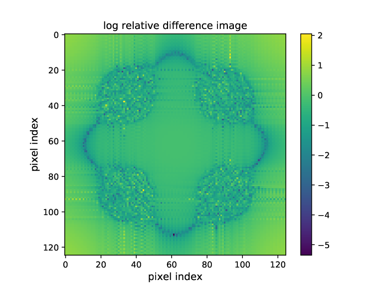
The previously cited work by Korkiakoski et al. [26] neglects interference effects when calculating the four pupil images. In the Fourier optics model presented here, the interference is treated automatically since all four beams are propagated simultaneously. In order to gain some understanding of the error due to neglecting interference between the two beams, we performed two simulations: In the first simulation, we utilized the full Fourier optics model, thereby creating (the "true" image). In the second simulation, we neglected interference, thereby creating (the "approximate" image). We produced the interference-free simulation by blocking transmission in 3 of the 4 pyramid faces and recording the intensity (which only had a single pupil image). One such image was created for each of the 4 pyramid surfaces, each in a different quadrant of the detector. Then, the 4 images were added to create the final, interference-free image . For this example, the Strehl ratio of the input beam was 0.3, and no noise was included.
The resulting images and were visually similar, but the mean of the ratio inside the pupil images was about 0.37. The results of this calculation are displayed in Fig. 2. The upper panel of Fig. 2 shows (normalized intensity units), and the lower panel displays the image of the log-ratio (). This result suggests that interference effects can be important and should not be neglected without justification.
5.2 Results: Regression Tests
The regressions were designed to compare the accuracy of the linear least-squares estimate of the phase of the field in the entrance pupil to the estimate made by nonlinear least-squares. The parameters varied for the different simulations runs were: the Strehl ratio of the input beam, the total number of photons entering the PyWFS, and the detector readout noise. The Strehl ratios for the input beam values were: , the total photon counts were , and the detector readout noise standard deviations were 0 and 4 counts/pixel. For each of these 60 parameter combinations, we performed 24 trials, each with randomly chosen input phases, shot noise and readout noise.
For the linearized least-squares estimator, the linearization point was taken to be a flat wavefront, so , resulting in an estimate . The starting point for the nonlinear estimator was , resulting in a new estimator . Both the linearized and nonlinear estimations forced the estimated phases to have zero-mean, as explained in Sec. 4.4.4. The enforcement of zero-mean removed the only zero (or small) singular value in the inversion problem (see Fig. 4), hence, there was no benefit to having a regularization parameter , and all of the estimators employed no regularization. Simulations not shown here confirmed that regularization (with the regularization matrix set to the identity, so ) provided no benefit to the accuracy of the estimators. (The only exception to this was cases at low Strehl ratio in which the unregularized estimator gain was negative. In these cases, a large regularization parameter drove the estimate towards 0, making the gain less negative.) The weight matrix in the cost functions, Eqs. (32) and (34), was set to the identity matrix. (Due to the very low intensity levels in some pixels of the detector, weighting of the measurements by the inverse of the variance noise caused poor performance of the algorithms. Finding an optimal weighting procedure was not explored.)
Fig. 6 shows the results of the various runs. The -axis of plots displays the RMS error of the estimates calculated as:
| (38) |
where "std" signifies standard deviation, where standard deviation is carried out over the 797 phase values. In each plot, the heavy black curve represents no gain, which is the error achieved by setting "estimated phase" to 0 in (38), thus any estimator below the curve is providing some information. Each data point shows the estimator error, according to (38), averaged over the 24 trials for a given parameter set. The data points have small horizontal offsets to alleviate visual over-crowding. The error bars, when large enough to be visible, indicate the standard deviation of this error over the 24 trials.
No estimator we used provided gain below a Strehl ratio of 0.1, due to the large nonlinearity error. This can be understood in terms of the amplification of nonlinear error upon inversion as explained in 44.1.2 and Fig. 5. For example, with a Strehl ratio of 0.1, photon counts and , the linearized estimator only provided a gain of . In this case, subsequently applying the BFGS algorithm resulted in a greatly decreased cost function. [In this case , but the gain achieved by the nonlinear estimate was .]
Varying the number of photons showed that photons is the lowest intensity level in which the regressions provided any gain (with zero readout noise) and represents something close to the lower limit at which the PyWFS simulated here can hope to operate. This seems reasonable, since ( photons)/(797 pupil pixels)photons/pixel corresponds to a signal-to-noise ratio of about . With a photon count of and counts/pixel, neither the linearized nor nonlinear estimator showed gain, and the results for these runs are not displayed.
The top panels in Fig. 6 show the results for photon counts of and , which are the lowest and the highest count rates we evaluated. For photon counts, the curves for readout noise levels of and counts/pixel are visually indistinguishable, so only the results for 4 counts/pixels are displayed. For the case of the photons, , the RMS error of the nonlinear estimator is too small to be seen on the plot at Strehl ratios of 0.7, 0.8 and 0.9. These values are , and , respectively, and the standard deviations of the RMS errors over the 24 runs are all about . These plots show that for photons, the nonlinear estimator begins to have an advantage over the linear estimator at a Strehl ratio of 0.3. The advantage continues to grow (the ratio of linear estimator error to the nonlinear estimator error increases) as the Strehl ratio increases. In contrast, the case of photons has such poor signal-to-noise, that there is little advantage to using the nonlinear estimator at any Strehl ratio.
The bottom panels in Fig. 6 show the results for photon counts and readout noise levels of 0 and 4 counts/pixel. The effect of the readout noise levels is clearly visible in the lower-right panel, where the Strehl ratio is greater than 0.5. In addition, the advantage of the nonlinear estimator over the linear one begins at a Strehl ratio of about 0.4. Unlike the case with photons, when only photons are available, the linear estimator performs almost as well as the nonlinear one at a Strehl ratio of 0.9. A similar effect can be seen in the upper panel for the photons case, were the linear estimator slightly outperforms the nonlinear estimator at a Strehl ratio of 0.9 (this was confirmed with several batches of 24 trials). The cause of this is the fact that the nonlinear cost function has many local minima and, when the data are noisy, the minimization algorithm finds a minimum that is not more desirable than the linearized least-squares solution. Why this effect is more pronounced at a Strehl ratio of 0.9 than Strehl ratios 0.3 through 0.8 is a bit of a curiosity. It is also interesting to note that performance of the estimators at Strehl ratios less than about 0.5 depends only weakly on the shot noise and detector noise. This is because the error in the solution is dominated by the nonlinearity, which is only partially mitigated by the nonlinear estimation method. At Strehl ratios of about 0.5 and above, the nonlinearity error is smaller, and the effects of noise are more pronounced.
6 Conclusions/Discussion
The desire to use the PyWFS without modulation stems from the high sensitivity of the device, but the price of this high sensitivity is nonlinearity. The simulation experiments here indicate that when the Strehl ratio of the input beam is above some threshold and the SNR is sufficient, nonlinear estimation methods can provide substantial advantages over linear estimation methods, thereby improving prospects for using the PyWFS without modulation. For the PyWFS simulated here, taking advantage of nonlinear estimation requires the input beam to have a Strehl ratio of about 0.3 or greater and photon flux about an order of magnitude greater than the operation threshold of the instrument. We have also shown that traditional slope-based measurements, in which the four PyWFS pupil images are reduced to two slope images, are unsuited to using the PYWFS without modulation. This is because the Jacobians associated with the slope representations of the measurements have steeper spectra of singular values than the Jacobians associated with the non-slope representations of the measurements. The effect of a steeper spectrum of singular values is more amplification of nonlinearity error and noise upon inversion, as explained in Sec. 44.1.2
We have argued that employing nonlinear estimators based on Newton and quasi-Newton methods for optimization should be possible for AO systems running at kHz rates for two reasons. Firstly, all detailed optical modeling is done beforehand, so no computationally expensive operations such as FFTs are required in real-time. With no real-time constraints on the optical modeling, one can apply almost any computational modeling method. Secondly, the computations required to obtain the modeled intensity and its derivatives can be carried out efficiently and in a massively parallel manner, as explained in Sec. 3. Using a computationally advantageous representation of the wavefront such as PhasePixel, as opposed to ModalPhase, reduces the real-time computational burden. Table 1 gives an approximate count of the required operations to calculate the intensity and its Hessian matrix at every detector pixel. For example, if specifying the model requires phase values and there are detector pixels at which the intensity and its derivatives are to be determined, calculating the intensity requires FLOPS, and calculating the intensity Jacobian requires an additional FLOPS. Calculating the Hessian matrix at every pixel is more expensive and requires an additional FLOPS, but there may be possibilities to reduce this by approximating these matrices with sparse alternatives, as explained in Sec. 33.3. In addition, every iteration of the optimization method will require more operations, as described in Sec. 44.3. For perspective, the NVIDIA Tesla P100 GPU Accelerator delivers 10 TeraFLOPs () of single-precision arithmetic per second, so a highly streamlined system with multiple GPUs may be capable of the required real-time computations.
This article has emphasized the nonlinearity of the non-modulated PyWFS and the fundamental challenges it imposes on estimation of the wavefront. The AO community has long recognized this challenge, and has used modulation of the input beam to make the PyWFS more linear. In order to mitigate some of the nonlinearity while retaining sensitivity, the PyWFS could be used with a small amount of modulation, and nonlinear estimation could be applied in such a situation as well. One obstacle to utilizing the estimation methods described here with a modulated PyWFS is increased computational expense of calculating the intensity and its derivatives. Let us take circular modulation applied by a steering mirror as an example. The tip/tilt applied by the steering mirror would need to be included in (14) and the equations that follow, until the intensity and its needed derivatives are determined. This would need to be done for multiple values of tip/tilt modulation in order to sample the path of the steering mirror. Then the intensities (and derivatives) would be averaged. Sampling the steering circle every 3.6 degrees would result in 100 times the computation of a calculation performed without modulation. One way that may reduce this burden would be to apply to use a spatial light modulator with, say, 10 modulation settings, in lieu of beam steering.[22, 23]
In both the modulated and non-modulated cases, determining the matrix , which is essentially a phase-accurate, calibrated computational model of the PyWFS, will be a challenge. Such an effort would likely require a combination of calibration measurements, and simulated propagation.
The impact of the nonlinear estimation methods described here on real-time, closed-loop control requires more detailed investigation. The next logical step would be end-to-end simulation in which the beam feeding the non-modulated PyWFS has been partially corrected by an upstream AO system.
The role of nonlinear estimation in post-analysis, where the time constraints are not as stringent, has not been mentioned. If data are acquired with sufficiently high Strehl ratio and signal-to-noise, this nonlinear estimation here should produce accurate estimates of the pupil phases and possibly the amplitudes as well. This capability would enable millisecond approaches to high-contrast imaging in which the wavefronts are needed as inputs to regression schemes. One such regression method produces simultaneous and self-consistent estimates of both the exoplanet image and the non-common path aberrations in the optics.[33]
Acknowledgments
The author thanks the referees, Olivier Guyon, and John Kohl for comments on the manuscript. This work has been supported by NSF Award #1600138 to the University of Michigan.
 |
 |
 |
 |
References
- [1] R. Ragazzoni, "Pupil plane wavefront sensing with an oscillating prism," Journal of Modern Optics 43, 289–293 (1996).
- [2] J. Wang, F. Bai, Y. Ning, L. Huang, and S. Wang, "Comparison between non-modulation four-sided and two-sided pyramid wavefront sensor," Optics Express 18, 27534–27549 (2010).
- [3] O. Fauvarque, B. Neichel, T. Fusco, and J.-F. Sauvage, "Variation around a pyramid theme: optical recombination and optimal use of photons," Opt. Lett. 40, 3528–3531 (2015).
- [4] O. Fauvarque, B. Neichel, T. Fusco, J.-F. Sauvage, and O. Girault, "General formalism for Fourier-based wave front sensing: application to the pyramid wave front sensors," Journal of Astronomical Telescopes, Instruments, and Systems 3, 019001 (2017).
- [5] M. van Kooten, J. P. Veran, and C. Bradley, "Alternative pyramid wavefront sensors," Journal of Astronomical Telescopes, Instruments, and Systems 3, 029001–029001 (2017).
- [6] R. Ragazzoni and J. Farinato, "Sensitivity of a pyramidic wave front sensor in closed loop adaptive optics," Astronomy and Astrophysics 350, L23–L26 (1999).
- [7] S. Esposito and A. Riccardi, "Pyramid Wavefront Sensor behavior in partial correction Adaptive Optic systems," Astronomy and Astrophysics 369, L9–L12 (2001).
- [8] T. Y. Chew, R. M. Clare, and R. G. Lane, "A comparison of the shack–hartmann and pyramid wavefront sensors," Optics Communications 268, 189–195 (2006).
- [9] V. Viotto, D. Magrin, M. Bergomi, M. Dima, J. Farinato, L. Marafatto, and R. Ragazzoni, "A study of pyramid wfs behaviour under imperfect illumination," in "Proc. Third AO4ELT Conf,", 38 (2013).
- [10] S. Esposito, A. Riccardi, L. Fini, A. T. Puglisi, E. Pinna, M. Xompero, R. Briguglio, F. Quirós-Pacheco, P. Stefanini, J. C. Guerra, L. Busoni, A. Tozzi, F. Pieralli, G. Agapito, G. Brusa-Zappellini, R. Demers, J. Brynnel, C. Arcidiacono, and P. Salinari, "First light AO (FLAO) system for LBT: final integration, acceptance test in Europe, and preliminary on-sky commissioning results," in "Adaptive Optics Systems II," Proc. SPIE 7736, 773609 (2010).
- [11] S. Esposito, A. Riccardi, E. Pinna, A. Puglisi, F. Quirós-Pacheco, C. Arcidiacono, M. Xompero, R. Briguglio, L. Busoni, L. Fini, "Natural guide star adaptive optics systems at lbt: Flao commissioning and science operations status," in Proc. SPIE, 84470U (2012).
- [12] K. M. Morzinski, L. M. Close, J. R. Males, D. Kopon, P. M. Hinz, S. Esposito, A. Riccardi, A. Puglisi, E. Pinna, R. Briguglio, "Magao: Status and on-sky performance of the magellan adaptive optics system," in Proc. SPIE, 914804 (2014).
- [13] N. Jovanovic, F. Martinache, O. Guyon, C. Clergeon, G. Singh, T. Kudo, V. Garrel, K. Newman, D. Doughty, J. Lozi, J. Males, Y. Minowa, Y. Hayano, N. Takato, J. Morino, J. Kuhn, E. Serabyn, B. Norris, P. Tuthill, G. Schworer, P. Stewart, L. Close, E. Huby, G. Perrin, S. Lacour, L. Gauchet, S. Vievard, N. Murakami, F. Oshiyama, N. Baba, T. Matsuo, J. Nishikawa, M. Tamura, O. Lai, F. Marchis, G. Duchene, T. Kotani, and J. Woillez, "The Subaru Coronagraphic Extreme Adaptive Optics System: Enabling High-Contrast Imaging on Solar-System Scales," Pub. Astron. Soc. Pacific 127, 890 (2015).
- [14] K. El Hadi, M. Vignaux, and T. Fusco, "Development of a pyramid wavefront sensor" in Proc. AO4ELT-III (2013).
- [15] R. A. Bernstein, P. J. McCarthy, K. Raybould, B. C. Bigelow, A. H. Bouchez, J. M. Filgueira, G. Jacoby, M. Johns, D. Sawyer, S. Shectman, "Overview and status of the giant magellan telescope project," in Proc. SPIE, 91451C (2014).
- [16] C. Boyer, "Adaptive optics program at tmt," in "Proc. Fourth AO4ELT Conf." (2015).
- [17] A. Burvall, E. Daly, S. R. Chamot, and C. Dainty, "Linearity of the pyramid wavefront sensor," Optics Express 14, 11925–11934 (2006).
- [18] C. Vérinaud, "On the nature of the measurements provided by a pyramid wave-front sensor," Optics Communications 233, 27–38 (2004).
- [19] O. Fauvarque, B. Neichel, T. Fusco, J.-F. Sauvage, and O. Girault, "General formalism for fourier-based wave front sensing," Optica 3, 1440–1452 (2016).
- [20] D. Greggio, D. Magrin, J. Farinato, R. Ragazzoni, M. Bergomi, M. Dima, L. Marafatto, and V. Viotto, "Avoiding to trade sensitivity for linearity in a real world wfs," in "Proc. Third AO4ELT Conf." (2013).
- [21] V. Viotto, M. Bergomi, M. Dima, J. Farinato, D. Greggio, D. Magrin, E. Portaluri, R. Ragazzoni, S. Esposito, and E. Pinna, "Pwfss on gmcao: a different approach to the non-linearity issue," in Proc. SPIE, 99096H (2016).
- [22] S. Wang, C. Rao, H. Xian, J. Zhang, J. Wang, and Z. Liu, "Laboratory demonstrations on a pyramid wavefront sensor without modulation for closed-loop adaptive optics system," Optics Express 19, 8135–8150 (2011).
- [23] V. Akondi, S. Castillo, and B. Vohnsen, "Digital pyramid wavefront sensor with tunable modulation," Optics Express 21, 18261–18272 (2013).
- [24] O. Guyon, "Limits of Adaptive Optics for High-Contrast Imaging," Astrophys. J. 629, 592–614 (2005).
- [25] J. R. Males, L. M. Close, O. Guyon, K. M. Morzinski, P. Hinz, S. Esposito, E. Pinna, M. Xompero, R. Briguglio, A. Riccardi, "The path to visible extreme adaptive optics with magao-2k and magao-x," in Proc. SPIE, 990952 (2016).
- [26] V. Korkiakoski, C. Vérinaud, M. Le Louarn, and R. Conan, "Comparison between a model-based and a conventional pyramid sensor reconstructor," Applied Optics 46, 6176–6184 (2007).
- [27] I. Shatokhina and R. Ramlau, "Convolution-and fourier-transform-based reconstructors for pyramid wavefront sensor," Applied Optics 56, 6381–6390 (2017).
- [28] J. W. Goodman, Introduction to Fourier Optics, second edition (The McGraw-Hill Companies, Inc., 1996).
- [29] J. Antichi, M. Munari, D. Magrin, and A. Riccardi, "Modeling pyramidal sensors in ray-tracing software by a suitable user-defined surface," Journal of Astronomical Telescopes, Instruments, and Systems 2, 028001 (2016).
- [30] T. K. Moon and W. C. Stirling, Mathematical Methods and Algorithms for Signal Processing (Prentice Hall, 2000).
- [31] D. P. Bertsekas, Nonlinear Programming: 3rd Edition (Athena Scientific, 2016).
- [32] B. D. Anderson and J. B. Moore, Optimal Filtering (Dover Publications, Inc., 1979).
- [33] R. A. Frazin, "Utilization of the Wavefront Sensor and Short-exposure Images for Simultaneous Estimation of Quasi-static Aberration and Exoplanet Intensity," Astrophys. J. 767, 21 (2013).