Specification-Driven Multi-Perspective
Predictive Business
Process Monitoring
(Extended Version)
Abstract
Predictive analysis in business process monitoring aims at forecasting the future information of a running business process. The prediction is typically made based on the model extracted from historical process execution logs (event logs). In practice, different business domains might require different kinds of predictions. Hence, it is important to have a means for properly specifying the desired prediction tasks, and a mechanism to deal with these various prediction tasks. Although there have been many studies in this area, they mostly focus on a specific prediction task. This work introduces a language for specifying the desired prediction tasks, and this language allows us to express various kinds of prediction tasks. This work also presents a mechanism for automatically creating the corresponding prediction model based on the given specification. Thus, different from previous studies, our approach enables us to deal with various kinds of prediction tasks based on the given specification. A prototype implementing our approach has been developed and experiments using a real-life event log have been conducted.
Keywords: Predictive Business Process Monitoring Prediction Task Specification Automatic Prediction Model Creation Multi-perspective Prediction
1 Introduction
Process mining [1] provides a collection of techniques for extracting process-related information from the logs of business process executions (event logs). One important area in this field is predictive business process monitoring, which aims at forecasting the future information of a running process based on the models extracted from event logs. Through predictive analysis, potential future problems can be detected and preventive actions can be taken in order to avoid unexpected situation (e.g., processing delay, SLA violations). Many techniques have been proposed for tackling various prediction tasks such as predicting the outcomes of a process [20, 13, 38, 27], predicting the remaining processing time [2, 37, 31, 29, 30], predicting the future events [14, 37, 15], etc (cf. [22, 23, 15, 34, 28, 6, 11]).
In practice, different business areas might need different kinds of prediction tasks. For instance, an online retail company might be interested in predicting the processing time until an order can be delivered to the customer, while for an insurance company, predicting the outcomes of an insurance claim process would be interesting. On the other hand, both of them might be interested in predicting whether their processes comply with some business constraints (e.g., the processing time must be finished within a certain amount of time).
When it comes to predicting the outcomes of a process or predicting an unexpected behaviour, it is important to specify the desired outcomes or the unexpected behaviour precisely. For instance, in the area of customer problem management, to increase customer satisfaction as well as to promote efficiency, we might be interested in predicting the possibility of “ping-pong behaviour” among the Customer Service (CS) officers while handling the customer problems. However, the definition of a ping-pong behaviour could be varied. For instance, when a CS officer transfers a customer problem into another CS officer who belongs to the same group, it can already be considered as a ping-pong behaviour since both of them should be able to handle the same problem. Another possible definition would be when a CS officer transfers a problem into another CS officer who has the same expertise, and the problem is transfered back into the original CS officer.
To have a suitable prediction service for our domain, we need to understand and specify the desired prediction tasks properly. Thus, we need a means to express the specification. Once we have characterized the prediction objectives and are able to express them properly, we need a mechanism to create the corresponding prediction model. To automate the prediction model creation, the specification should be machine processable. As illustrated above, such specification mechanism should also allow us to specify some constraints over the data, and compare some data values at different time points. For example, to characterize the ping-pong behaviour, one possibility is to specify the behaviour as follows: “there is an event at a certain time point in which the CS officer is different with the CS officer in the event at the next time point, but both of them belong to the same group”. Note that here we need to compare the information about the CS officer names and groups at different time points.
In this work, we tackle those problems by providing the following contributions:
(i) We introduce a rich language for expressing the desired prediction tasks. This language allows us to specify various kinds of prediction tasks. In some sense, this language also allows us to specify how to create the desired prediction models based on the event logs. (ii) We devise a mechanism for building the corresponding prediction model based on the given specification. Once created, the prediction model can be used to provide predictive analysis service in business process monitoring. (iii) We exhibit how our approach can be used for tackling various kinds of prediction tasks (cf. Section 3.3). (iv) We develop a prototype that implements our approach and enables the automatic creation of prediction models based on the specified prediction objective. (v) To demonstrate the applicability of our approach, we carry out experiments using a real-life event log that was provided for the BPI Challenge 2013 [36].Roughly speaking, in our approach, we specify various desired prediction tasks by specifying how we want to map each (partial) business processes execution information into the expected predicted information. Based on this specification, we automatically train either classification or regression models that will serve as the prediction models. By specifying a set of desired prediction tasks, we can obtain multi-perspective prediction services that enable us to focus on various aspects and predict various information. Our approach is independent with respect to the classification/regression model that is used. In our implementation, to get the expected quality of predictions, the users are allowed to choose the desired classification/regression model as well as the feature encoding mechanisms (to allow some sort of feature engineering). This paper is the extended version of [33] and it provides supplementary materials for [33] by providing more explanations, examples and experiments.
2 Preliminaries
This section provides some background concepts for the rest of the paper.
Trace, Event and Event Log. We follow the usual notion of event logs as in process mining [1]. An event log captures historical information about the execution of business processes. In an event log, each execution of a process is represented as a trace. Each trace has several events, and each event in the trace captures the information about a particular event that happens during the process execution. Events are characterized by various attributes, e.g., timestamp (the time at which the event occurred).
Let be the event universe (i.e., the set of all event identifiers), and be the set of attribute names. For any event , and attribute name , denotes the value of the attribute of . E.g., denotes the timestamp of the event . If an event does not have an attribute named , then (undefined value). A finite sequence over of length is a mapping , and such a sequence is represented as a tuple of elements of , i.e., where for . The set of all finite sequences over is denoted by . The length of a sequence is denoted by .
A trace is a finite sequence over such that each event occurs at most once in , i.e., and for , we have , where refers to the event of the trace at the index . Let be a trace, denotes the -length prefix of (for ). For example, let , is an example of a trace, , and . Finally, an event log is a set of traces such that each event occurs at most once in the entire log, i.e., for each such that , we have that , where .
An IEEE standard for representing event logs, called XES (eXtensible Event Stream), has been introduced in [18]. The standard defines the XML format for organizing the structure of traces, events and attributes in event logs. It also introduces some extensions that define some attributes with pre-defined meaning such as:
(i) “concept:name”, which stores the name of event/trace; (ii) “org:resource”, which stores the name/identifier of the resource that triggered the event (e.g., a person name); (iii) “org:group”, which stores the group name of the resource that triggered the event.Classification and Regression. In machine learning [24], a classification and regression model can be seen as a function that takes some input features/variables and predicts the corresponding target value/output . The key difference is that the output range of the classification task is a finite number of discrete categories (qualitative outputs) while the output range of the regression task is continous values (quantitative outputs) [17, 16]. Both of them are supervised machine learning techniques where the models are trained with labelled data. I.e., the inputs for the training are the pairs of input variables and target value . This way, the models learn how to map certain inputs into the expected target value .
3 Approach
Our approach for obtaining a predictive process monitoring service consists of the following main steps:
(i) specify the desired prediction tasks and (ii) automatically create the prediction model based on the given specification.Once created, we can use the models to predict the future information. In the following, we elaborate these steps.
3.1 Specifying the Desired Prediction Tasks
This section explains the mechanism for specifying the desired prediction task. Here we introduce a language that is able to capture the desired prediction task in terms of the specification on how to map each (partial) trace in the event log into the desired prediction results. Such specification can be used to train a classification/regression model that will be used as the prediction model.
In our approach, the specification of a particular prediction task is specified as an analytic rule, where an analytic rule is an expression of the form
Each in is called condition expression, while and are called target expression (for ). We explain and formalize how to specify a condition and target expression after providing some intuitions below.
An analytic rule will be interpreted as a function that maps (partial) traces into the values obtained from evaluating the target expressions. The mapping is based on the condition that is satisfied by the corresponding trace. Let be a (partial) trace, such function can be illustrated as follows (the formal definition will be given later):
We will see that a target expression essentially specifies the desired prediction result or expresses the way how to compute the desired prediction result. Thus, an analytic rule can also be seen as a means to map (partial) traces into the desired prediction results, or to compute the expected prediction results of (partial) traces.
To specify a condition expression in analytic rules, we introduce a language called First-Order Event Expression (FOE). Roughly speaking, an FOE formula is a First-Order Logic (FOL) formula [35] where the atoms are expressions over some event attribute values and some comparison operators (e.g., , , ). Moreover, the quantification in FOE is restricted to the indices of events (so as to quantify the time points). The idea of condition expressions is to capture a certain property of (partial) traces. To give some intuition, before we formally define the language, consider the ping-pong behaviour that can be specified as follows:
where “” is an expression for getting the “org:group” attribute value of the event at the index . The formula basically says that “there exists a time point i that is bigger than the current time point (i.e., in the future), in which the resource (the person in charge) is different with the resource at the time point (i.e., the next time point), their groups are the same, and the next time point is still not later than the last time point”. As for the target expression, some simple examples would be some strings such as “Ping-Pong” and “Not Ping-Pong”. Based on these, we can create an example of analytic rule
where is as above. In this case, specifies a task for predicting the ping-pong behaviour. In the prediction model creation phase, we will create a classifier that classifies (partial) traces based on whether they satisfy or not. During the prediction phase, such classifier can be used to predict whether a given (partial) trace will lead into ping-pong behaviour or not.
The target expression can be more complex than merely a string. For instance, it can be an expression that involves arithmetic operations over numeric values such as
which computes “the time difference between the timestamp of the last event and the current event (i.e., remaining processing time)”. Then we can create an analytic rule
,
which specifies a task for predicting the remaining time, because will map each (partial) trace into its remaining processing time. In this case, we will create a regression model for predicting the remaining processing time of a given (partial) trace. Section 3.3 provides more examples of prediction tasks specification using our language.
Formalizing the Condition and Target Expressions. As we have seen in the examples above, we need to refer to a particular index of an event within a trace. To capture this, we introduce the notion of index expression defined as follows:
where
(i) is an index variable. (ii) pintis a positive integer (i.e., ). (iii) and are special indices in which the former refers to the index of the last event in a trace, and the latter refers to the index of the current event (i.e., last event of the trace prefix under consideration). For instance, given a -length prefix of the trace , is equal to (or ), and is equal to . (iv) and are the usual arithmetic addition and subtraction operation over indices.The semantics of index expression is defined over -length trace prefixes. Since an index expression can be a variable, given a -length trace prefix of the trace , we first introduce a variable valuation , i.e., a mapping from index variables into . Then, we assign meaning to index expression by associating to and an interpretation function which maps an index expression into . Formally, is inductively defined as follows:
To access the value of an event attribute, we introduce event attribute accessor, which is an expression of the form
where attName is an attribute name and is an index expression. To define the semantics of event attribute accessor, we extend the definition of our interpretation function such that it interprets an event attribute accessor expression into the attribute value of the corresponding event at the given index. Formally, is defined as follows:
E.g., “” refers to the value of the attribute “org:resource” of the event at the position .
The value of an event attribute can be either numeric (e.g., 26, 3.86) or non-numeric (e.g., “sendOrder”), and we might want to specify properties that involve arithmetic operations over numeric values. Thus, we introduce the notion of numeric expression and non-numeric expression as expressions defined as follows:
where
(i) and are the usual boolean values, (ii) is the usual string, (iii) is real numbers, (iv) (resp. ) is event attribute accessor for accessing an attribute with non-numeric values (resp. numeric values), (v) and are the usual arithmetic operations over numeric expressions.To give the semantics for numeric expression and non-numeric expression, we extend the definition of our interpretation function by interpreting , , , and as themselves (e.g., , ), and by interpreting the arithmetic operations as usual, i.e., for the addition operator we have
The definition is similar for the subtraction operator. Note that the value of an event attribute might be undefined . In this work, we define that the arithmetic operations involving give (e.g., ).
We are now ready to specify the notion of event expression as follows:
where
(i) lcopstands for a logical comparison operator ( or ). (ii) acopstands for an arithmetic comparison operator (, , , , or ).We interpret each logical/arithmetic comparison operator as usual (e.g., is interpreted as true, “receivedOrder” “sendOrder” is interpreted as false). It is easy to see how to extend the definition of our interpretation function towards interpreting event expressions, therefore we omit the details.
Finally, we are ready to define the language for specifying condition expression, namely First-Order Event Expression (FOE). An FOE formula is a First Order Logic (FOL) formula where the atoms are event expressions and the quantification is ranging over event indices. Syntactically FOE is defined as follows:
Where is an event expression. The semantics of FOE constructs is based on the usual FOL semantics. Formally, given a -length trace prefix of the trace , and index variables valuation , we extend the definition of our interpretation function as follows11 1 We assume that variables are standardized apart, i.e., no two quantifiers bind the same variable (e.g., ), and no variable occurs both free and bound (e.g., ). As usual in FOL, every FOE formula can be transformed into a semantically equivalent formula where the variables are standardized apart by applying some variable renaming [35].:
note that stands for a new index variable valuation obtained from as follows:
Intuitively, substitutes each variable with , while the other variables are substituted the same way as is defined. The semantics of and is as usual in FOL. When is a closed formula, its truth value does not depend on the valuation for the index variables, and we denote the interpretation of simply by . We also say that satisfies , written , if .
Finally, the condition expression in analytic rules is specified as closed FOE formulas, while the target expression is specified as either numeric expression or non-numeric expression, except that target expressions are not allowed to have index variables (Thus, they do not need variable valuation).
Essentially, FOE has the following main features:
(i) it allows us to specify constraints over the data; (ii) it allows us to (universally/existentially) quantify different event time points and to compare different event attribute values at different event time points; (iii) it supports arithmetic expressions/operations over the data.Checking Whether a Condition Expression is Satisfied. Given a -length trace prefix of the trace , and a condition expression (which is expressed as an FOE formula), to explain how to check whether , we first introduce some properties of FOE formula below. Let be an FOE formula, we write to denote a new formula obtained by substituting each variable in by .
Theorem 3.1
Given an FOE formula , and a -length trace prefix of the trace ,
Proof (sketch)
By the semantics definition, satisfies iff there exists an index , such that satisfies the formula that is obtained from by substituting each variable in with . Thus, it is the same as satisfying the disjunction of formulas that is obtained by considering all possible substitutions of the variable in (i.e., ). This is the case because such disjunction of formulas will be satisfied by when there is a formula in the disjunction that is satisfied by . ∎
Theorem 3.2
Given an FOE formula , and a -length trace prefix of the trace ,
Proof (sketch)
Similar to Theorem 3.1, except that we use conjunctions of formulas. ∎
To check whether , we perform the following three steps:
(1) Eliminate all quantifiers. This can be easily done by applying Theorems 3.1 and 3.2. As a result, each variable will be instantiated with a concrete value. (2) Evaluate each event attribute accessor expression based on the event attributes in . From this step, we will have a formula which is constituted by only concrete values composed by logical/comparison/arithmetic operators. (3) Last, we evaluate all logical, arithmetic and comparison operators.Formalizing the Analytic Rule. With this machinery in hand, now we can formalize the semantics of analytic rules as introduced above. Formally, given an analytic rule
is interpreted as a function that maps (partial) traces into the values obtained from evaluating the target expressions defined below
where is -length trace prefix of the trace , and recall that is the application of our interpretation function to the target expression in order to evaluate the expression and get the value. Checking whether can be done as explained above. We also require that an analytic rule to be coherent, i.e., all target expressions of an analytic rule should be either only numeric or non-numeric expressions. An analytic rule in which all of its target expressions are numeric expressions is called numeric analytic rule , while an analytic rule in which all of its target expressions are non-numeric expressions is called non-numeric analytic rule .
Given a -length trace prefix and an analytic rule , we say that is well-defined for if maps into exactly one target value, i.e., for every condition expressions and in which and , we have that . The notion of well-defined can be generalized to event logs. Given an event log and an analytic rule , we say that is well-defined for if for each possible -length trace prefix of each trace in , we have that is well-defined for . This condition can be easily checked for the given event log and an analytic rule .
Note that our notion of well-defined is more relaxed than requiring that each condition must not be overlapped, and this gives flexibility for making a specification using our language. For instance, one can specify several characteristics of ping-pong behaviour in a more convenient way by specifying several conditional-target rules (i.e., , ) instead of using disjunctions of these several characteristics. From now on we only consider the analytic rules that are coherent and well-defined for the event logs under consideration.
3.2 Building the Prediction Model
Given an analytic rule and an event log , if is a numeric analytic rule, we build a regression model. Otherwise, if is a non-numeric analytic rule, we build a classification model. Note that our aim is to create a prediction function that takes (partial) traces as inputs. Thus, we train a classification/regression function in which the inputs are the features obtained from the encoding of trace prefixes in the event log (the training data). There are several ways to encode (partial) traces into input features for training a machine learning model. For instance, [19] studies various encoding techniques such as index-based encoding, boolean encoding, etc. In [37], the authors use the so-called one-hot encoding of event names, and also add some time features (e.g., the time increase with respect to the previous event). In general, an encoding technique can be seen as a function that takes a trace as the input and produces a set of features (i.e., ).
In our approach, users are allowed to choose the desired encoding mechanism by specifying a set of preferred encoding functions (i.e., ). This allows us to do some sort of feature engineering (note that the desired feature engineering approach, that might help increasing the prediction performance, can also be added as one of these encoding functions). The set of features of a trace is then obtained by combining all features produced by applying each of the selected encoding functions into the corresponding trace. In the implementation (cf. Section 4), we provide some encoding functions that can be selected in order to encode a trace.
Input:
an analytic rule , an event log , a set of encoding
functions
Output: a prediction function
Algorithm 1 illustrates how to build the prediction model based on the given inputs, namely:
(i) an analytic rule , (ii) an event log , and (iii) a set of encoding functions.The algorithm works as follows: for each -length trace prefix of each trace in the event log (where ), we do the following:
In line 3, we apply each encoding function into , and combine all obtained features. This step gives us the encoded trace prefix. In line 4, we compute the expected prediction result (target value) by applying the analytical rule to . In line 5, we add a new training instance by specifying that the prediction function maps the encoded trace prefix into the target value computed in the previous step. Finally, we train the prediction function and get the desired prediction function.3.3 Showcase of Our Approach: Multi-Perspective Predictive Analysis Service
An analytic rule specifies a particular prediction task of interest. To specify several desired prediction tasks, we only have to specify several analytic rules, i.e., . Given a set of analytic rules, i.e., , our approach allows us to construct a prediction model for each analytic rule . This way, we can get a multi-perspective prediction analysis service provided by all of the constructed prediction models where each of them focus on a particular prediction objective.
In Section 3.1 we have seen the examples of prediction task specification for predicting the ping-pong behaviour and the remaining processing time. In the following, we show other examples of specifying prediction task using our language.
Predicting unexpected behaviour. We can specify a task for predicting unexpected behaviour by first expressing the characteristics of the unexpected behaviour. The condition expression (in Section 3.1) expresses a possible characteristic of ping-pong behaviour. Another possible characterization of this behaviour is shown below:
essentially, characterizes the condition where “an officer transfers a task into another officer of the same group, and then the task is transfered back into the original officer”. In the event log, this situation is captured by the changes of the org:resource value in the next event, but then it changes back into the original value in the next two events, while the values of org:group remain the same. We can then specify an analytic rule for specifying the ping-pong behaviour prediction task as follows:
Based on Algorithm 1, during the training phase, maps each trace prefix that satisfies either or into the target value “Ping-Pong”, and those prefixes that neither satisfy nor into “Not Ping-Pong”. After the training based on this rule, we get a classifier that is trained for distinguishing between (partial) traces that will and will not lead into ping-pong behaviour. This example also exhibits the ability of our language to specify a behaviour that has multiple characteristics.
Predicting next event. The task for predicting the next event is specified as follows: . In the training phase, maps each -length trace prefix into its next event name, because “” is evaluated into the name of the event at the index (i.e., ). If , then maps into (undefined). After the training, we get a classifier that is trained to give the next event name of the given (partial) trace.
Predicting the next event timestamp. This task can be specified as follows:22 2 Note that timestamp can be represented as milliseconds since epoch (hence, it is a number).
.
maps each -length trace prefix into the next event timestamp. Hence, we train a regression model that outputs the next event timestamp of the given (partial) trace.
Predicting SLA/business constraints compliance. Using FOE, we can easily specify expressive SLA conditions/business constraints, and automatically create the corresponding prediction model using our approach. E.g., we can specify a constraint:
which essentially says “whenever there is an event where an order is created, eventually there will be an event where the order is delivered and the time difference between the two events (the processing time) is less than 10.800.000 milliseconds (3 hours)”.
4 Implementation and Experiment
As a proof of concept, by using Java and WEKA, we have implemented a prototype33 3 More information about the implementation architecture, the code, the tool, and the screencast can be found at http://bit.ly/predictive-analysis. that is also a ProM44 4 ProM is an extendable framework for process mining (http://www.promtools.org). plug-in. The prototype includes a parser for our language and a program for automatically processing the specification as well as building the corresponding prediction model based on the approach explained in Sections 3.1 and 3.2. We also provide several feature encoding functions to be selected such as one hot encoding of attributes, time since the previous event, time since midnight, attribute values encoding, etc. We can also choose the desired machine learning model to be built.
Our experiments aim at showing the applicability of our approach in automatically constructing reliable prediction models based on the given specification. The experiments were conducted using the real life event log from BPI Challenge 2013 (BPIC 13) [36]. For the experiment, we use the first 2/3 of the log for the training and the last 1/3 of the log for the testing. In BPIC 13, the ping-pong behaviour among support teams is one of the problems to be analyzed. Ideally a customer problem should be solved without involving too many support teams. Here we specify a prediction task for predicting the ping-pong behaviour by first characterizing a ping-pong behaviour among support teams as follows:
Roughly, says that there is a change in the support team while the problem is not being “Queued”. We then specify the following analytic rule:
that can be fed into our tool for obtaining the prediction model. For this case, we automatically generate Decision Tree and Random Forest models from that specification. We also predict the time until the next event by specifying the following analytic rule:
For this case, we automatically generate Linear Regression and Random Forest models.
We evaluate the prediction performance of each -length prefix of each trace in the testing set (for ). We use accuracy and AUC (Area Under the ROC Curve) [16] values as the metrics to evaluate the ping-pong prediction. For the prediction of the time until the next event, we use MAE (Mean Absolute Error) [16], and RMSE (Root Mean Square Error) [16] values as the metrics, and we also provide the MAE and RMSE values for the mean-based prediction (i.e., the basic approach where the prediction is based on the mean of the target values in the training data). The results are summarized in Tables 2 and 1. We highlight the evaluation for several prediction points, namely
(i) early prediction (at the 1/4 of the trace length), (ii) intermediate prediction (at the 1/2 of the trace length), and (iii) late prediction (at the 3/4 of the trace length).The column “All” presents the aggregate evaluation for all -length prefix where .
| Accuracy | AUC value | |||||||
| Early | Mid | Late | All | Early | Mid | Late | All | |
| Decision Tree | 0.82 | 0.67 | 0.87 | 0.77 | 0.76 | 0.69 | 0.63 | 0.75 |
| Random Forest | 0.83 | 0.73 | 0.91 | 0.83 | 0.89 | 0.73 | 0.78 | 0.87 |
| MAE (in days) | RMSE (in days) | |||||||
| Early | Mid | Late | All | Early | Mid | Late | All | |
| Linear Regression | 0.70 | 1.42 | 2.64 | 2.07 | 1.04 | 1.87 | 2.99 | 2.77 |
| Random Forest | 0.34 | 1.07 | 1.81 | 1.51 | 1.03 | 2.33 | 2.89 | 2.61 |
| Mean-based Prediction | 2.42 | 2.33 | 2.87 | 2.70 | 2.44 | 2.40 | 3.16 | 2.90 |
The AUC values in Table 1 show that our approach is able to automatically produce reasonable prediction models (The AUC values ). Table 2 shows that all of the automatically generated models perform better than the mean-based prediction (the baseline). The experiment also exhibits that the performance of our approach depends on the machine learning model that is generated (e.g., in Table 1, random forest performs better than decision tree). Since our approach does not rely on a particular machine learning model, it justifies that we can simply plug in different supervised machine learning techniques in order to get different/better performance. In the future we plan to experiment with deep learning approach in order to get a better accuracy. As reported by [37], the usage of LSTM neural networks could improve the accuracy of some prediction tasks. More experiments can be seen in Appendix 0.C.
5 Related Work
This work is related to the area of predictive analysis in business process management. In the literature, there have been several works focusing on predicting time-related properties of running processes. For instance, the works in [2, 31, 29, 30] focus on predicting the remaining processing time. The works by [34, 23, 28] focus on predicting delays in process execution. The authors of [37] present a deep learning approach for predicting the timestamp of the next event and use it to predict the remaining cycle time. Looking at another perspective, the works by [20, 13, 38] focus on predicting the outcomes of a running process. The work by [20] introduces a framework for predicting the business constraints compliance of a running process. In [20], the business constraints are formulated in propositional Linear Temporal Logic (LTL), where the atomic propositions are all possible events during the process executions. Another work on outcomes prediction is presented by [27], which proposes an approach for predicting aggregate process outcomes by also taking into account the evaluation of process risk. Related to process risks, [11] proposes an approach for risks prediction. Another stream of works tackle the problem of predicting the future events of a running process (cf. [37, 30, 15, 14, 6]).
A key difference between those works and ours is that, instead of focusing on a specific prediction task, this work enables us to specify and focus on various prediction tasks. To deal with these various desired prediction tasks, we also present a mechanism that can automatically build the corresponding prediction models based on the given specification of prediction tasks.
This work is also related to the works on devising specification language. Unlike the propositional LTL, which is the basis of Declare language [26] and typically used for specifying business constraints over sequence of events (cf. [20]), our FOE language (which is part of our rule-based specification language) allows us not only to specify properties over sequence of events but also to specify properties over the data (attribute values) of the events. Concerning data-aware specification language, the work by [3] introduces a data-aware specification language by combining data querying mechanisms and temporal logic. Such language has been used in verification of data-aware processes systems (cf. [4, 10, 7, 32, 9, 8]). The works by [12, 21] enrich the Declare language with data conditions based on First-Order LTL (LTL-FO). Although those languages are data-aware, they do not support arithmetic expressions/operations over the data which is absolutely needed, e.g., for expressing the time difference between the timestamp of the first and the last event. Another interesting data-aware language is S-FEEL, which is part of the Decision Model and Notation (DMN) standard [25] by OMG. Though S-FEEL supports arithmetic expressions over the data, it does not allow us to (universally/existentially) quantify different event time points and to compare different event attribute values at different event time points, which is needed, e.g., in the ping-pong behaviour specification. Importantly, our language is specifically tuned for expressing data-aware properties based on the typical structure of event logs, and the design is highly driven by the typical prediction tasks in business process management.
6 Discussion and Conclusion
We have introduced a mechanism for specifying the desired prediction tasks by using a rule-based language, and for automatically creating the corresponding prediction models based on the given specification. A prototype of ProM plug-in that implements our approach has been developed and several experiments using a real life event log confirmed the applicability of our approach.
Future work includes the extension of the tool and the language. One possible extension would be to incorporate aggregate functions such as SUM and CONCAT. These functions enable us to specify more tasks such as the prediction of total cost that is based on the sum of the cost attributes in all events. The CONCAT function could allow us to specify the prediction of the next sequence of activities by concatenating all next activities. We would also like to extend the language with trace attribute accessor that allows us to specify properties involving trace attribute values. There is also a possibility to exploit existing logic-based tools such as Satisfiability Modulo Theories (SMT) solver [5] for performing reasoning tasks related to the language. Experimenting with other supervised machine learning techniques would be the next step as well, e.g., using deep learning approach in order to improve accuracy.
Acknowledgement. This research has been supported by the Euregio IPN12 “KAOS: Knowledge-Aware Operational Support” project, which is funded by the “European Region Tyrol-South Tyrol-Trentino” (EGTC) under the first call for basic research projects. The author thanks Tri Kurniawan Wijaya for various suggestions on this work, and Yasmin Khairina for the implementation of some prototype components. The author acknowledges the support of the Faculty of Computer Science of the Free University of Bozen-Bolzano, where he is staying for an extended research visit.
References
- [1] van der Aalst, W.M.P.: Process Mining - Data Science in Action. Springer, 2nd edn. (2016)
- [2] van der Aalst, W.M.P., Schonenberg, M., Song, M.: Time prediction based on process mining. Information Systems 36(2), 450 – 475 (2011)
- [3] Bagheri Hariri, B., Calvanese, D., De Giacomo, G., Deutsch, A., Montali, M.: Verification of relational data-centric dynamic systems with external services. In: the 32nd ACM SIGACT SIGMOD SIGAI Symp. on Principles of Database Systems (PODS). pp. 163–174 (2013)
- [4] Bagheri Hariri, B., Calvanese, D., Montali, M., Santoso, A., Solomakhin, D.: Verification of semantically-enhanced artifact systems. In: Proc. of the 11th Int. Joint Conf. on Service Oriented Computing (ICSOC). LNCS, vol. 8274, pp. 600–607. Springer (2013)
- [5] Barrett, C.W., Sebastiani, R., Seshia, S.A., Tinelli, C.: Satisfiability modulo theories. In: Biere, A., Heule, M., & van Maaren, H. (Eds.), Handbook of Satisfiability. IOS Press (2009)
- [6] Breuker, D., Matzner, M., Delfmann, P., Becker, J.: Comprehensible predictive models for business processes. MIS Quarterly 40(4) (2016)
- [7] Calvanese, D., Ceylan, İ.İ., Montali, M., Santoso, A.: Verification of context-sensitive knowledge and action bases. In: Proc. of the 14th Eur. Conf. on Logics in Artificial Intelligence (JELIA). LNCS, vol. 8761, pp. 514–528. Springer (2014)
- [8] Calvanese, D., De Giacomo, G., Lembo, D., Montali, M., Santoso, A.: Ontology-based governance of data-aware processes. In: Proc. of the 6th Int. Conf. on Web Reasoning and Rule Systems (RR). LNCS, vol. 7497, pp. 25–41. Springer (2012)
- [9] Calvanese, D., Montali, M., Santoso, A.: Verification of generalized inconsistency-aware knowledge and action bases. In: Proc. of the 24th Int. Joint Conf. on Artificial Intelligence (IJCAI). pp. 2847–2853. AAAI Press (2015)
- [10] Calvanese, D., Montali, M., Santoso, A.: Verification of generalized inconsistency-aware knowledge and action bases (extended version). CoRR Technical Report arXiv:1504.08108, arXiv.org e-Print archive (2015), available at http://arxiv.org/abs/1504.08108
- [11] Conforti, R., de Leoni, M., La Rosa, M., van der Aalst, W.M., ter Hofstede, A.H.: A recommendation system for predicting risks across multiple business process instances. Decision Support System 69, 1 – 19 (2015)
- [12] De Masellis, R., Maggi, F.M., Montali, M.: Monitoring data-aware business constraints with finite state automata. In: Proc. of the 2014 Int. Conf. on Software and System Process. pp. 134–143. ACM (2014)
- [13] Di Francescomarino, C., Dumas, M., Maggi, F.M., Teinemaa, I.: Clustering-based predictive process monitoring. IEEE Trans. on Serv. Comput. PP(99), 1–18 (2016)
- [14] Di Francescomarino, C., Ghidini, C., Maggi, F.M., Petrucci, G., Yeshchenko, A.: An eye into the future: Leveraging a-priori knowledge in predictive business process monitoring. In: Proc. of the 15th Int. Conf. on Business Process Management (BPM). LNCS, vol. 10445, pp. 252–268. Springer (2017)
- [15] Evermann, J., Rehse, J.R., Fettke, P.: Predicting process behaviour using deep learning. Decision Support System 100, 129 – 140 (2017)
- [16] Friedman, J., Hastie, T., Tibshirani, R.: The elements of statistical learning. Springer (2001)
- [17] Han, J., Pei, J., Kamber, M.: Data mining: concepts and techniques. Elsevier (2011)
- [18] IEEE Comp. Intelligence Society: IEEE Standard for eXtensible Event Stream (XES) for achieving interoperability in event logs and event streams. IEEE Std 1849-2016 (2016)
- [19] Leontjeva, A., Conforti, R., Di Francescomarino, C., Dumas, M., Maggi, F.M.: Complex symbolic sequence encodings for predictive monitoring of business processes. In: Proc. of the 13th Int. Conf. on Business Process Management (BPM). LNCS, vol. 9253, pp. 297–313. Springer (2015)
- [20] Maggi, F.M., Di Francescomarino, C., Dumas, M., Ghidini, C.: Predictive monitoring of business processes. In: Proc. of the 26th Int. Conf. on Advanced Information Systems Engineering (CAiSE). LNCS, vol. 8484, pp. 457–472. Springer (2014)
- [21] Maggi, F.M., Dumas, M., García-Bañuelos, L., Montali, M.: Discovering data-aware declarative process models from event logs. In: Proc. of the 11th Int. Conf. on Business Process Management (BPM). pp. 81–96. Springer (2013)
- [22] Metzger, A., Leitner, P., Ivanović, D., Schmieders, E., Franklin, R., Carro, M., Dustdar, S., Pohl, K.: Comparing and combining predictive business process monitoring techniques. IEEE Trans. on Systems, Man and Cybernetics: Systems 45(2), 276–290 (2015)
- [23] Metzger, A., Franklin, R., Engel, Y.: Predictive monitoring of heterogeneous service-oriented business networks: The transport and logistics case. In: Annual SRII Global Conf. 2012. pp. 313–322 (2012)
- [24] Mohri, M., Rostamizadeh, A., Talwalkar, A.: Foundations of machine learning. MIT press (2012)
- [25] Object Management Group: Decision Model and Notation (DMN) 1.0 (2015), http://www.omg.org/spec/DMN/1.0/
- [26] Pesic, M., van der Aalst, W.M.P.: A declarative approach for flexible business processes management. In: BPM Workshops 2006. pp. 169–180. Springer (2006)
- [27] Pika, A., van der Aalst, W., Wynn, M., Fidge, C., ter Hofstede, A.: Evaluating and predicting overall process risk using event logs. Information Sciences 352-353, 98 – 120 (2016)
- [28] Pika, A., van der Aalst, W.M.P., Fidge, C.J., ter Hofstede, A.H.M., Wynn, M.T.: Predicting deadline transgressions using event logs. In: BPM Workshops 2012. LNBIP, vol. 132, pp. 211–216. Springer (2012)
- [29] Polato, M., Sperduti, A., Burattin, A., de Leoni, M.: Data-aware remaining time prediction of business process instances. In: 2014 Int. Joint Conf. on Neural Networks (IJCNN). pp. 816–823 (2014)
- [30] Polato, M., Sperduti, A., Burattin, A., de Leoni, M.: Time and activity sequence prediction of business process instances. CoRR abs/1602.07566 (2016)
- [31] Rogge-Solti, A., Weske, M.: Prediction of remaining service execution time using stochastic petri nets with arbitrary firing delays. In: Proc. of the 11th Int. Joint Conf. on Service Oriented Computing (ICSOC). LNCS, vol. 8274, pp. 389–403. Springer (2013)
- [32] Santoso, A.: Verification of Data-aware Business Processes in the Presence of Ontologies. Ph.D. thesis, Free University of Bozen-Bolzano, Technische Universität Dresden (2016), http://nbn-resolving.de/urn:nbn:de:bsz:14-qucosa-213372
- [33] Santoso, A.: Specification-driven multi-perspective predictive business process monitoring. In: Enterprise, Business-Process and Information Systems Modeling, BPMDS 2018, EMMSAD 2018. LNBIP, vol. 318, pp. 97–113. Springer (2018)
- [34] Senderovich, A., Weidlich, M., Gal, A., Mandelbaum, A.: Queue mining – predicting delays in service processes. In: Proc. of the 26th Int. Conf. on Advanced Information Systems Engineering (CAiSE). LNCS, vol. 8484, pp. 42–57. Springer (2014)
- [35] Smullyan, R.M.: First Order Logic. Springer, Berlin (Germany) (1968)
- [36] Steeman, W.: BPI challenge 2013 (2013), https://doi.org/10.4121/uuid:a7ce5c55-03a7-4583-b855-98b86e1a2b07
- [37] Tax, N., Verenich, I., La Rosa, M., Dumas, M.: Predictive business process monitoring with LSTM neural networks. In: Proc. of the 29th Int. Conf. on Advanced Information Systems Engineering (CAiSE). LNCS, vol. 10253, pp. 477–492. Springer (2017)
- [38] Verenich, I., Dumas, M., La Rosa, M., Maggi, F.M., Di Francescomarino, C.: Complex symbolic sequence clustering and multiple classifiers for predictive process monitoring. In: BPM Workshops 2015. LNBIP, vol. 256, pp. 218–229. Springer (2015)
Appendix 0.A More Showcases of Our Approach
Previously, we have seen some examples of prediction task specification using our language (cf. Sections 3.1, 3.3 and 4). In the following, more examples on prediction tasks specification are presented.
0.A.1 Predicting Process Performance
One can consider the processes that take more than certain amount of time as “slow process” while the other are considered “normal”. Given a (partial) process execution information (trace), it might be interesting to predict whether it will end up as a slow process or a normal process. This prediction task can be specified as follows:
.
where
.
Essentially, states that if the total running time of a trace is greater than 18.000.000 milliseconds (5 hours), then it is categorized as “slow”. In the training phase, maps each -length trace prefix into the corresponding performance category (i.e., “slow” or “normal”) of the corresponding process represented by . This way, we get a prediction model that is trained to predict whether a certain (partial) trace will give slow performance, or it will be normal.
Notice that one can defined more fine-grained characteristic of process performance. For instance, we can add one more process characteristic into by saying that those processes that spend less than 3 hours (10.800.000 milliseconds) are considered as “fast”. This is specified by as follows:
.
where
.
.
0.A.2 Predicting Delay
Delay can be defined as the condition when the actual processing time is longer that the expected processing time. Suppose we have the information about the expected processing time, e.g., provided by an attribute “expectedDuration” of the first event, we can specify an analytic rule for predicting the delay as follows:
.
where
.
essentially says that the difference between the last event timestamp and the first event timestamp (i.e., the processing time) is greater than the expected duration (provided by the value of the event attribute “expectedDuration”). maps each trace prefix into either “Delay” or “normal” depending on whether the processing time of the whole trace is greater than the expected processing time or not. After the training phase using this rule, we get a classifier that is trained to distinguish between the partial traces that (probably) will and will not lead into a delay situation.
0.A.3 Predicting SLA/Business Constraints Compliance
We have seen some prediction task specification examples for predicting the compliance of SLA/business constraints. Another example of an SLA would be a requirement which states that each activity must be finished within 2 hours. This condition can be expressed as follows:
We can then specify an analytic rule for predicting the compliance of this SLA as follows:
.
Notice that we can express the same specification in a different way, for instance
.
where
Essentially states that there exists a timepoint , in which is still not after the last time point and the difference between the timestamp of the event at and is greater than 120.000 milliseconds (2 hours). Using either or , our algorithm for building the prediction model (cf. Algorithm 1) gives us a classifier that is trained to distinguish between the partial traces that (probably will) comply and not comply with this SLA.
0.A.4 Predicting The Next Lifecycle
The task for predicting the lifecycle can be specified as follows:
.
In the training phase, maps each -length trace prefix into its next lifecycle, because “” is evaluated into the lifecycle information of the event at the index (i.e., ). If , then maps into (undefined). After the training, we get a classifier that is trained to give the information about the most probable next lifecycle of the given partial trace.
Appendix 0.B Implementation
Our approach is visually described in Figure 1. Essentially, it consists of two main phases, namely the preparation and the prediction phases. In the preparation phase, we construct the prediction models based on the given event log, as well as based on:
(i) the prediction tasks specification, (ii) the desired encoding mechanisms, and (iii) the desired classification/regression models.Once the prediction models are built, in the second phase, we can use the generated models to perform the prediction task in order to predict the future information of the given partial trace.
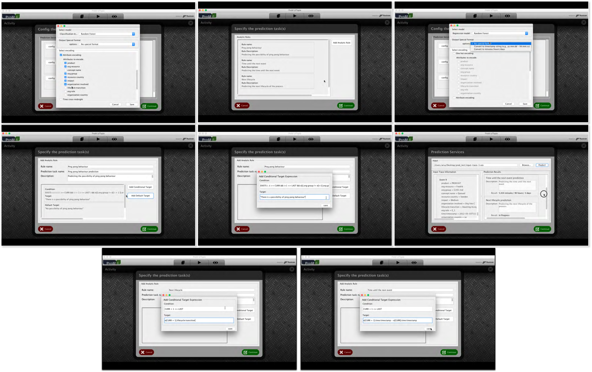
As a proof of concept, we have implemented two ProM plug-ins. One plug-in is for synthesizing the prediction models based on the given specification, and another plug-in is for predicting the future information of a partial trace by using the generated prediction models. Some screenshots of our ProM plug-ins are depicted in Figure 2. The screencast of our plug-ins can be found at http://bit.ly/predictive-analysis.
Appendix 0.C More Experiments
We perform more experiments on the tasks that were presented in Section 4 (i.e., the prediction of ping-pong behaviour among support teams and the time until the next event). Additionally, we also conduct an experiment on another characterization of ping-pong behaviour, namely the ping-pong behaviour among the officers in the same group. Apart from aiming at showing the applicability of our approach in automatically constructing reliable prediction models based on the given specification, we also conduct experiments on different types of encoding techniques in order to see how it would affect the quality of the prediction results in our approach.
One encoding technique that we use is one-hot encoding. The notion of one-hot encoding is as usual (cf. [14, 37, 30]), except that we are not only considering the one-hot encoding of the activity/event name (i.e., the attribute “concept:name”), but we allow the possibility of adding the one-hot encoding of another event attribute (e.g., “lifecycle:transition”). In the prototype tool that we have developed, when we want to use one-hot encoding, the users can select the corresponding event attribute. We briefly explain the notion of one-hot encoding as follows: Let be an event attribute name, be the set of all possible values of the attribute attName, and be an ordering function over the set of all possible values of attName such that if and only if (for each ). The one-hot encoding of the attribute attName that has the value is a binary vector of length where all components are set to 0, except that the component of at the index is set to 1.
We also consider the encoding in which we directly add the value of an event attribute as a feature. Here, this type of encoding is called attribute encoding. Similar to one-hot encoding, we can select the attribute in which we want to apply the attribute encoding. Note that, in some sense, the attribute encoding allows us to do an encoding that is similar to the index-based encoding that was studied in [19].
0.C.1 Predicting the Ping-pong Behaviour
The experiment of predicting the ping-pong behaviour in Section 4 uses the one-hot encoding of the attribute concept:name, the attribute encoding of “org:resource”, “org:group”, “lifecycle:transition”, “organization involved”, “impact”, “product”, “resource country”, “organization country”, and “org:role”. Here we report another experiments on this problem, where we use different types of encodings. The results are summarized in Tables 3, 4, 5, 6 and 7 (For all of these experiments we add the encoding of time features, namely the time since midnight, the time since the previous event, the time since the first day of the week).
| Accuracy | AUC value | |||||||
|---|---|---|---|---|---|---|---|---|
| Early | Mid | Late | All | Early | Mid | Late | All | |
| Decision Tree | 0.73 | 0.49 | 0.93 | 0.71 | 0.51 | 0.30 | 0.43 | 0.67 |
| Random Forest | 0.72 | 0.46 | 0.76 | 0.68 | 0.54 | 0.36 | 0.40 | 0.68 |
| Accuracy | AUC value | |||||||
|---|---|---|---|---|---|---|---|---|
| Early | Mid | Late | All | Early | Mid | Late | All | |
| Decision Tree | 0.15 | 0.81 | 0.94 | 0.77 | 0.50 | 0.50 | 0.50 | 0.50 |
| Random Forest | 0.73 | 0.49 | 0.93 | 0.71 | 0.51 | 0.29 | 0.35 | 0.67 |
| Accuracy | AUC value | |||||||
|---|---|---|---|---|---|---|---|---|
| Early | Mid | Late | All | Early | Mid | Late | All | |
| Decision Tree | 0.74 | 0.49 | 0.88 | 0.70 | 0.51 | 0.40 | 0.54 | 0.71 |
| Random Forest | 0.74 | 0.48 | 0.80 | 0.69 | 0.56 | 0.39 | 0.50 | 0.70 |
| Accuracy | AUC value | |||||||
|---|---|---|---|---|---|---|---|---|
| Early | Mid | Late | All | Early | Mid | Late | All | |
| Decision Tree | 0.75 | 0.48 | 0.91 | 0.71 | 0.54 | 0.35 | 0.48 | 0.69 |
| Random Forest | 0.74 | 0.48 | 0.80 | 0.69 | 0.58 | 0.40 | 0.48 | 0.70 |
| Accuracy | AUC value | |||||||
|---|---|---|---|---|---|---|---|---|
| Early | Mid | Late | All | Early | Mid | Late | All | |
| Decision Tree | 0.83 | 0.67 | 0.87 | 0.78 | 0.77 | 0.71 | 0.69 | 0.76 |
| Random Forest | 0.82 | 0.73 | 0.91 | 0.83 | 0.90 | 0.72 | 0.78 | 0.87 |
0.C.2 Predicting the Time Until the Next Event
The experiment of predicting the time until the next event in Section 4 uses the one-hot encoding of the attribute concept:name, the attribute encoding of “org:resource”, “org:group”, “lifecycle:transition”, “organization involved”, “impact”, “product”, “resource country”, “organization country”, and “org:role”. Here we report another experiments on this problem, where we use different types of encoding techniques. The results are summarized in Tables 8, 9, 10, 11 and 12 (For all of these experiments we add the encoding of time features, namely the time since midnight, the time since the previous event, the time since the first day of the week).
| MAE (in days) | RMSE (in days) | |||||||
|---|---|---|---|---|---|---|---|---|
| Early | Mid | Late | All | Early | Mid | Late | All | |
| Linear Regression | 0.64 | 1.40 | 2.74 | 2.06 | 1.02 | 1.80 | 3.05 | 2.59 |
| Random Forest | 0.75 | 1.48 | 2.80 | 2.21 | 2.02 | 2.66 | 4.25 | 3.74 |
| Mean-based Prediction | 2.42 | 2.33 | 2.87 | 2.70 | 2.44 | 2.40 | 3.16 | 2.90 |
| MAE (in days) | RMSE (in days) | |||||||
|---|---|---|---|---|---|---|---|---|
| Early | Mid | Late | All | Early | Mid | Late | All | |
| Linear Regression | 1.25 | 1.75 | 3.03 | 2.41 | 1.33 | 1.93 | 3.52 | 2.82 |
| Random Forest | 0.70 | 1.57 | 2.88 | 2.24 | 2.03 | 2.85 | 4.08 | 3.69 |
| Mean-based Prediction | 2.42 | 2.33 | 2.87 | 2.70 | 2.44 | 2.40 | 3.16 | 2.90 |
| MAE (in days) | RMSE (in days) | |||||||
|---|---|---|---|---|---|---|---|---|
| Early | Mid | Late | All | Early | Mid | Late | All | |
| Linear Regression | 0.61 | 1.35 | 2.30 | 1.96 | 0.92 | 1.77 | 2.59 | 2.56 |
| Random Forest | 0.70 | 1.42 | 2.61 | 2.11 | 1.75 | 2.48 | 3.58 | 3.35 |
| Mean-based Prediction | 2.42 | 2.33 | 2.87 | 2.70 | 2.44 | 2.40 | 3.16 | 2.90 |
| MAE (in days) | RMSE (in days) | |||||||
|---|---|---|---|---|---|---|---|---|
| Early | Mid | Late | All | Early | Mid | Late | All | |
| Linear Regression | 0.84 | 1.36 | 2.78 | 2.22 | 0.94 | 1.66 | 3.34 | 2.71 |
| Random Forest | 0.63 | 1.36 | 2.56 | 2.10 | 1.70 | 2.51 | 3.68 | 3.46 |
| Mean-based Prediction | 2.42 | 2.33 | 2.87 | 2.70 | 2.44 | 2.40 | 3.16 | 2.90 |
| MAE (in days) | RMSE (in days) | |||||||
|---|---|---|---|---|---|---|---|---|
| Early | Mid | Late | All | Early | Mid | Late | All | |
| Linear Regression | 0.71 | 1.44 | 2.82 | 2.15 | 1.02 | 1.88 | 3.22 | 2.87 |
| Random Forest | 0.32 | 1.11 | 2.02 | 1.61 | 0.84 | 2.29 | 3.04 | 2.70 |
| Mean-based Prediction | 2.42 | 2.33 | 2.87 | 2.70 | 2.44 | 2.40 | 3.16 | 2.90 |
0.C.3 Predicting The Ping-pong Behaviour Among Officers in the Same Group
We also experiment with another characterization of ping-pong behaviour, namely the ping-pong behaviour among the officers in the same group. The behaviour is specified as follows:
The results are summarized in Tables 13 and 14 (For all of these experiments we add the encoding of time features, namely the time since midnight, the time since the previous event, the time since the first day of the week). .
| Accuracy | AUC value | |||||||
|---|---|---|---|---|---|---|---|---|
| Early | Mid | Late | All | Early | Mid | Late | All | |
| Decision Tree | 0.95 | 0.97 | 0.97 | 0.97 | 0.57 | 0.67 | 0.61 | 0.63 |
| Random Forest | 0.96 | 0.99 | 0.99 | 0.99 | 0.71 | 0.79 | 0.90 | 0.81 |
| Accuracy | AUC value | |||||||
|---|---|---|---|---|---|---|---|---|
| Early | Mid | Late | All | Early | Mid | Late | All | |
| Decision Tree | 0.96 | 0.98 | 0.98 | 0.98 | 0.80 | 0.77 | 0.75 | 0.78 |
| Random Forest | 0.96 | 0.99 | 0.99 | 0.99 | 0.74 | 0.87 | 0.92 | 0.84 |
0.C.4 Observations
For the prediction of the time until the next event, the results in Tables 12 and 2 show us that encoding the value of the attribute “concept:name” using one-hot encoding gives us a better performance. However, it is not the case for the prediction of ping-pong behaviour among officers in the same group. Tables 13 and 14 show that the encoding of the “concept:name” value using attribute encoding gives us a slightly better performance (in particular, see the AUC values). For the prediction of ping-pong behaviour among support teams, the results do not show a big different whether we encode the value of the attribute “concept:name” using one-hot encoding or attribute encoding (cf. Tables 1 and 7). On the other hand, looking at Tables 3, 4, 5 and 6 as well as Tables 1 and 7, we see that the more features that we use, the better performance that we get. However, it is not always be the case, as it is exhibited by the experiments on predicting the time until the next event. A conclusion that we can draw from these facts is that the choice of encodings certainly influence the quality of the prediction, and based on those experiments, there is no encoding that is always better than the others. For instance, although one-hot encoding seems to give more fine-grained information in the encoding, the experiments show that encoding the information using one-hot encoding does not always give a better result. Hence, it justifies the importance of our approach for allowing the user to choose the desired encoding mechanism that is more suitable for their problem.
Additionally, the experiments also show that, with a suitable choice of encoding mechanisms, our approach is able to automatically synthesize reliable prediction models based on the given specification (i.e., for the classification case, the AUC values are greater than 0.5, and for the regression case, the results are better than the mean-based prediction). Thus, it confirms the applicability of our proposed approach in performing predictive process monitoring tasks based on the given specification.