Adiabatic invariant analysis of dark and dark-bright soliton stripes in two-dimensional Bose-Einstein condensates
Abstract
In the present work, we develop an adiabatic invariant approach for the evolution of quasi-one-dimensional (stripe) solitons embedded in a two-dimensional Bose-Einstein condensate. The results of the theory are obtained both for the one-component case of dark soliton stripes, as well as for the considerably more involved case of the two-component dark-bright (alias “filled dark”) soliton stripes. In both cases, analytical predictions regarding the stability and dynamics of these structures are obtained. One of our main findings is the determination of the instability modes of the waves as a function of the parameters of the system (such as the trap strength and the chemical potential). Our analytical predictions are favorably compared with results of direct numerical simulations.
pacs
75.50.Lk, 75.40.Mg, 05.50.+q, 64.60.-iI Introduction
A theme of wide interest over the last two decades is the study of dark solitons; relevant explorations were physically motivated in nonlinear optics [1] and more recently have been broadly extended to atomic Bose-Einstein condensates (BECs) [2]. One of their two-dimensional (2D) generalizations, i.e., vortices —which play a prominent role in nonlinear field theory [3]— have also attracted attention in nonlinear optics [4, 5] and atomic BECs [6, 7]. These two structures are intimately connected through their topological nature: vortices can be thought of as a 2D “incarnation” of a dark soliton —possessing a phase winding. However, there is also an important link from the point of view of stability analysis, namely dark solitons become unstable in higher dimensions [8, 9], giving indeed rise to vortices. The relevant dynamics is characterized by the manifestation of the so-called transverse (or “snaking”) instability, which leads to the undulation and the eventual breakup of dark solitons into multi-vortex patterns. This feature has been used experimentally since early on as a means of producing vortices, both in optics [10] and in BECs [11], and has been a subject of continuing theoretical interest [12, 13, 14]. Mechanisms on how to avoid the instability have also been explored (see, e.g., Ref. [15]).
In the recent work of Ref. [14], we developed an approach to tackle transverse instabilities, with a special emphasis on the case examples of ring dark solitons (studied in optics [16, 17, 18] and BECs [19, 20, 21]) and spherical shell solitons (also of wide interest in the same areas [16, 22, 23, 24]). The technique was based on a generalization of the adiabatic invariant (or so-called “Landau dynamics”) approach. This was a technique earlier utilized for dark solitons in one-dimensional (1D) settings [25, 26] and for ring dark solitons in quasi-1D ones [27].
Our scope in the present work is to extend the relevant considerations to the case of the dark soliton stripe for the one-component case, as well as the dark-bright (alias “filled dark”) soliton stripe in the case of two-component systems of the nonlinear Schrödinger (NLS) type. We develop, in both cases, the adiabatic invariant theory —extending it in this way to the multi-component, multi-dimensional case— and derive the equations of motion of these “solitonic filaments”, in the presence of curvature, as well as in that of the external potential relevant to BECs. Subsequently, from these 1D partial differential equations (PDEs) characterizing the -position of the filament as a function of , assuming that the filament extends along the -direction, we infer the equilibrium states, i.e., the homogeneous equilibria corresponding to straight filaments. We linearize around these equilibria to identify their modes of potential instability and their corresponding wavenumbers as a function of parameters, such as the chemical potential of the system. Finally, we test all of the above existence, stability, and dynamical predictions against numerical simulations, finding good agreement with the corresponding PDE results (both analytical ones —e.g., for the linearization— and lower-dimensional, effective dynamical ones).
Our presentation is structured as follows. First, we give a summary of our analytical results both for the single- and for the two-component case. Then, we proceed to test the conclusions of our analysis against the stability analysis and dynamics of the original, full 2D, PDE. Finally, we summarize our findings and present a number of possibilities for future work.
II Mathematical Formulation and Analytical Results
II.1 One-Component Case
Our starting point is the dimensionless 1D NLS equation —also referred to as the Gross-Pitaevskii (GP) equation— which includes the external trapping potential , appearing generically in the BEC context; the equation is of the form:
| (1) |
For the derivation of both the 1D and 2D models used herein in their dimensionless form (from their dimensional variants), the reader can consult, e.g., Ref. [28]. In the absence of external potential, , and for a background density (equal to the chemical potential) , the conserved energy assumes the form:
In the same case (where the potential is absent), Eq. (1) possesses a dark soliton solution, of position and velocity , given by:
| (2) |
with . For this solution, the energy yields: . We then follow Refs. [25, 26] and use this energy as an adiabatic invariant (AI) —i.e., an invariant under slow variations— in the presence of a slowly-varying potential . This is justified by the consideration that, in this case, the background density will be slowly-varying according to the transformation . Therefore, assuming the AI of this quantity, we obtain
| (3) |
which gives, after taking a time derivative, the following equation of motion for the dark soliton position:
| (4) |
This result, obtained originally in Ref. [29] and retrieved in Ref. [25], is well-known to be in very good agreement with numerical results for large [25, 26, 28]. In this limit, the dark solitons can be thought of as particles bearing no internal structure, enabling the application of this effective particle theory.
Our considerations are geared towards generalizing the above ideas to 2D. Let us then consider the 2D NLS equation:
| (5) |
where, importantly, we consider the case corresponding to only trapping along the (longitudinal) -direction. This 2D NLS conserves the Hamiltonian:
Now, assuming an ansatz of the form (2) with the center position not solely a function of , but also a function of the transverse variable , i.e., , we are able to describe solutions of the form of a dark soliton stripe, or soliton filament, that runs along the -direction. Evaluating the 2D Hamiltonian for this dark soliton stripe yields an “effective energy” (an AI again) of the form:
| (6) |
Here, the transverse energy contribution (corresponding to the term) has been accounted for through the term proportional to . One can try to obtain various pieces of quantitative information based on this “effective Hamiltonian” describing the transverse motion of the soliton filament. Similarly to the 1D case, we take and integrating by parts along the -direction (and considering localization of the solution along the -direction, so that partial derivatives with respect to at are zero), we obtain the following effective PDE for the dark soliton filament’s dynamical evolution:
| (7) |
where and . One can then make the following relevant observations regarding this novel emerging PDE model:
- (i)
For weak undulations, and in the absence of the potential, the dynamics is described by
yielding the proper linear growth rate of the transverse instability [8]. Note that such an instability for dark solitons is only present in the elliptic dispersion case [dispersion term equals to , as in the case under consideration].
- (ii)
- (iii)
It is possible to obtain existence and stability information for the dark soliton stripe. A particularly interesting example, even at the linear setting, concerns the case with the —generic for BECs— 1D parabolic trap . This case concerns a 1D dark-soliton embedded in a longitudinal trap, while the transverse direction remains untrapped. Naturally, is the stationary state, corresponding to a dark soliton stripe located at the potential minimum. Applying the normal mode ansatz and ignoring higher orders of , yields the following eigenvalues (or eigenfrequencies ):
(8) where and is the length of the transverse direction (extending from to ). Importantly, this is a prediction suggesting the presence (for large chemical potential ) of a large number of unstable eigendirections whose growth rate is explicitly given by Eq. (8). Note that in the large chemical potential limit, grows proportionally to . Hence, we obtain both explicit analytical predictions, such as Eq. (8), and the simpler (in that they reduce the dimensionality from 2D to 1D for the evolution of the soliton filament) effective PDE model (7) that can be compared to the full numerical computations.
II.2 Two-Component Case
We now turn to the case of the dark-bright (DB) soliton stripes, which are two-component structures that can be viewed as “filled” dark soliton stripes. DB solitons in quasi-1D BECs, first predicted theoretically in Ref. [30] and then studied in a series of experiments (in two- and recently generalized in three-components) [31, 32, 33, 34, 35, 36, 37, 38], feature a rather intuitive physical premise: the dark solitons operate as an effective potential well, trapping a bright soliton in the second component, even though this latter structure is not possible (by itself, i.e., in a single-component setting) for a self-defocusing nonlinearity [39].
In the 1D case of the so-called Manakov model of equal interaction coefficients (a very realistic case in settings such as hyperfine states of 87Rb [30]), the equations for the components and , confined respectively by the potentials and , read:
| (9) |
In this case, in the absence of external potentials, , the solution for the DB soliton is of the form:
| (10) | |||||
| (11) |
where suitable algebraic conditions connect the soliton parameters such as the chemical potentials and , the speed related parameter , the DB soliton center position and the inverse width , and , the norm of the solution (corresponding to number of particles in the bright component) in the -component [30].
In 1D, the DB free energy can then be approximated as [30]:
where . Similarly to the case of the dark soliton stripe, let us now consider a DB soliton filament described by its position . Hence, assuming and and accounting for the transverse contribution to the energy, , yields the 2D free energy:
| (12) |
where now and the potential terms are evaluated at . The resulting equation of motion for the DB filament with longitudinal profile given by Eqs. (10) and (11) is obtained from by integrating along the -direction. The resulting effective 1D PDE for is particularly lengthy and has the following form:
| (13) | |||||
Nonetheless, linearizing around the fixed point which bears no -dependence, using , we obtain the following dynamical equation for perturbations around the stationary (straight) filament:
with (squared) eigenfrequencies
where now , and all potentials (and their derivatives) are evaluated at . For the experimentally relevant case of a parabolic trap [39], we have , , and , leading to:
| (14) |
We can now make the following relevant observations regarding the eigenfrequencies given in Eq. (14):
- (i)
- (ii)
The third term is the transverse undulation frequency contribution from a flat background (in the transverse direction). Together, the first and third term combine to yield the result of Eq. (8) for the undulation in a 1D trap of the 2D dark soliton stripe.
- (iii)
Finally, the fourth term corresponds to the contribution to the 2D transverse undulation stemming from the bright soliton.
An appealing feature of this step-by-step approach is that one not only obtains an expression for the spectral mode eigenfrequencies, but also an intuitive sense on the nature and origin of each contribution.
Having explored both the nonlinear (fully dynamical) and the linear (spectral) setup of such a multi-component soliton filament, it is natural to examine how these conclusions fare against the full numerical computations of the original 2D model of Eq. (5).
III Numerical Methods and Findings
III.1 General setup and methodology
In our numerical simulations, we consider the full 2D dimensionless GP equations (5) and (9) for the one- and two-component cases, respectively. We consider a trapping potential acting only along the -direction, namely:
| (15) |
and we consider periodic boundary conditions along the -direction. As for the trap strength, we use —without loss of qualitative generality of our results— for all of the following numerical computations.
Our numerical simulations consist of the following serial steps: we first solve for stationary states and compute their linear stability spectrum, and, finally, we explore their dynamics. Because the system has -translational symmetry (due to the form of the potential and its associated steady states), we solve the stationary states only along the -direction to obtain the cross section of the sought-for 2D steady states.
Furthermore, to render the 2D stability computations more efficient, we use the fact that our solutions are -independent in order to extract the linear stability eigenvalues as a collection of 1D eigenvalue problems using basis expansions, also called the partial wave method. This technique is summarized in Refs. [23, 40] for one- and two-component radially symmetric BECs. The method can be straightforwardly tailored in a similar manner to our setting by replacing the angular direction with (and expressing the Laplacian in rectangular coordinates rather than polar). Since the methods are fairly similar, we refer the interested reader to Refs. [23, 40] for more details. Nonetheless, we briefly mention here that the method computes eigenvalues for each -mode separately (in our case or , and eigenvalues of and are complex conjugates) and the full 2D spectrum is simply the union of all the individual 1D spectra.
In our computations, we use the domain which is sufficiently long to support the background cloud carrying the dark and dark-bright solutions, and we use chemical potentials up to . We have checked that the domain size along the -direction (provided it is large enough to support the background cloud) does not affect the numerical results hereby presented. In Fig. 1 we depict a typical example (in the case of large chemical potentials) for the dark and dark-bright soliton states.

In what follows, we span the spectra of the original NLS model using the lowest modes, as in Ref. [14]. In our simulations, a typical lattice spacing for the finite difference method is , and in certain cases, a small spacing as low as was required to achieve spectrum convergence at high densities. The full PDE dynamics were performed using a standard second order finite differencing in space combined with a forward fourth-order Runge-Kutta in time.


III.2 NLS and AI spectra
Now that we are equipped with the reduced AI PDEs (7) and (13) for the dark and the DB solitons for one- and two-components, respectively, let us corroborate the validity of this reduction approach at the level of the associated spectra for stationary states. Thus, we numerically compute the spectra for the dark and DB solitons as the chemical potential is varied starting from the linear limit. The dark soliton emerges from the linear limit at as it is the first excited state of the (1D) quantum harmonic oscillator. Similarly, the DB soliton emerges from the linear limit at and corresponding to coupling the first excited state and the ground state of the quantum harmonic oscillator. We follow the dark soliton steady state configuration and its corresponding spectrum using continuation starting from the linear limit () up to .
The spectra for both the NLS model (1) and our analytical prediction (8) for the effective AI reduction are depicted in Fig. 2, for two values of the transverse length : the top panel corresponds to a relatively small , while the bottom panel corresponds to . As expected, the stability properties of the dark soliton stripe strongly depend on the domain’s transverse length . In particular, a larger number of instabilities are observed for larger values of since larger domains can support instabilities with shorter wavenumbers. However, more importantly, we observe that the NLS and AI spectra agree reasonably well, with better agreement for larger chemical potential . Moreover, the lower frequency (and/or growth rate) modes converge well for smaller chemical potentials, while the larger frequency (and growth rate) modes are progressively better for higher chemical potentials.


Figure 3 depicts a similar scenario to the dark soliton stripe presented in Fig. 2, but now for the DB soliton stripe. In this case, we start from the linear limit and progress with a linear “trajectory” in the parameter space until reaching . As before, there is a very good agreement between the full NLS spectrum and the analytical prediction (14) computed from the AI reduction.
It is interesting to note that, despite the strong instabilities present at high densities, both dark and DB soliton stripes can be stable sufficiently close to the linear limit. This stabilization is due to the finite size of the domain in the -direction, where small enough wavenumbers will not be able to fit in the domain. For instance, when , the dark soliton stripe does not acquire an unstable eigenvalue until reaching . In fact, we have checked numerically that full (2D) time integration of the stationary dark soliton stripe for is indeed stable for long times (results not shown here). Similarly, the spectrum for the DB soliton stripe suggests that this configuration [for the choice of parameters described above] is stable for [along the aforementioned parameter trajectory]. We have also verified, by direct integration, that the DB soliton stripe for is indeed stable for long times (results not shown here). For both simulations we added to the exact stationary stripe states a relatively small random perturbation (on the order of ), and no visible instability growth was observed for times up to .
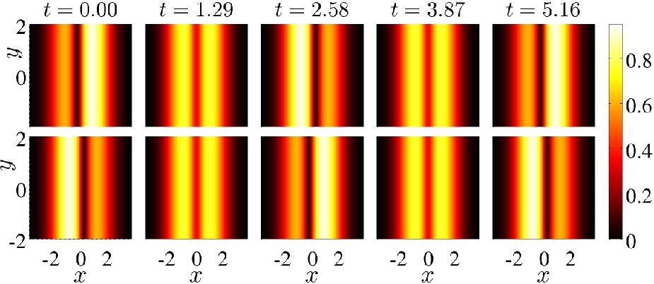
The stability for small enough values of the chemical potential (and/or small enough domain lengths ) can be used to stabilize additional solutions. For instance, it is possible to stabilize two-component breathing dark-dark soliton stripes, resulting from a SO(2) rotation of DB soliton stripes, similarly to the quasi-1D case [36, 37, 41]. These solutions are based on two coupled dark solitons with different chemical potentials, . An example of such a stable breathing dark-dark soliton stripe is depicted in Fig. 4, with the top and bottom panels showing each of the two components. It is observed that the two dark soliton stripes start from different sides of the trap, pass through each other, and oscillate back to restart the cycle. We have checked that, indeed, this oscillating pattern is stable and that the oscillation period is indeed determined by the chemical potential imbalance , namely (cf. Ref. [41] for details on the derivation of this result).


III.3 NLS and AI dynamics
In this last section, we compare the evolutionary dynamics for dark and DB soliton stripes obtained through the AI reduction and the original NLS model.
First, we compare the dynamics of the dark soliton stripe, as described by the AI reduction and obtained by the original NLS model. For all the comparisons presented below we chose a relatively large chemical potential for the dark component; recall that for this relatively large value of the chemical potential, we concluded that there is a good match between the corresponding spectra of the AI reduction and of the NLS model. Furthermore, in order to keep at bay the amount of instabilities that can be present in the system, we use a relatively small transverse length of for which only a limited number of instabilities are present (see the previous section for details).
To initialize the system we consider a dark soliton stripe initially displaced in the -direction by and perturbed in the (transverse) -direction by harmonic undulations of amplitude . To be more specific, this amounts to a filament with initial position given by , and with zero initial velocity; in what follows we use , , and for all of our numerics. This initial perturbation is intended to seed a specific destabilization eigendirection for best comparison between the AI and NLS models. Choosing random initial perturbations along the -direction results in similar destabilizations along the most unstable eigendirection, but the precise timing and the location (along the -axis) of the unstable mode obviously depend on each realization; thus, a match between the AI and NLS models is less straightforward to achieve. Since the initial condition does not correspond to a steady state, and since we do not have access to the exact left-to-right oscillatory solution of a dark, or DB, soliton, we initialize the NLS model with the corresponding displaced (to ) exact solution (found in the absence of external potential, ) with a local chemical potential adjusted to , as per the adiabatic invariant approach.
In general, we expect the evolution of the stripes to adhere to two principal features:
- (i)
the left-to-right oscillations —with frequencies for the dark soliton and the corresponding adjusted frequency (14) due to the presence of the bright soliton components for the DB soliton— and
- (ii)
the destabilization of the stripe through the perturbed -th undulation mode (if it is indeed unstable).
The former trait, for our choice of , leads to a left-to-right oscillation period of around . In contrast, note that the instabilities —see spectra of the previous section— have typical values of order one when divided by . In fact, the instabilities for large scale precisely as and, thus, for the chosen relatively large chemical value of , the instabilities will grow proportional to . Therefore, the growth of instabilities will be typically much faster than the left-to-right oscillations and thus the latter oscillations will not be typically observable within the time range of our simulations focusing on the growth of the instabilities.


Figure 5 depicts two examples for the destabilization of the dark soliton stripe through the (top set of panels) and (bottom set of panels) modes. As expected, the left-to-right oscillation of the dark soliton stripe is barely visible while the stripe suffers a strong instability along the and modes. This instability is responsible for spatial undulations that the dark soliton filament develops, the so-called snaking, along the -direction. As the snaking intensifies, the filament breaks up into pairs of vortices (see dark spots in the field’s modulus and the phase jump singularities in the field’s phase). In fact, pairs of vortices are created when perturbing with the -th mode. More importantly, the figure shows that the reduced dynamical AI model (7) is able to qualitatively and quantitatively describe the full NLS evolution of Eq. (1) before the filament breakup into vortex pairs. Note that the AI approach displays a slightly faster instability growth rate when compared to the original NLS dynamics. This is straightforwardly understandable as the AI spectra predicts slightly larger real parts for the eigenvalues when compared to the original NLS dynamics (see, for instance, the top panel in Fig. 2). Also notice that the AI results are not shown past the time when the filament starts to develop the vortex pairs. At that point, the AI PDE solution develops singularities (vertical slope) and its numerical evolution breaks down. This is of course natural as, by construction, our AI dynamics:
- (i)
does not allow for bends of the filament leading to multi-valuedness of the filament’s location , and
- (ii)
as the original NLS filament starts breaking up into vortex pairs, the assumption that the solution remains as a longitudinal dark soliton filament is clearly violated.
Nonetheless, it is remarkable that the lower dimensional AI reduction is able to qualitatively, and, where appropriate, even quantitatively, capture the soliton filament dynamics before its breakup into vortex pairs.
In Fig. 6 we present results similar to the ones presented in Fig. 5, but for the DB soliton stripe. The conclusions stated above also apply to this more complex case, where our AI approach is able to capture the snaking of the DB soliton filament before its breakup into vortex pairs in the dark component filled by bright cores in the other component. The latter vortex-bright single and pair structures have also been previously examined; see, e.g., Refs. [42, 43] and references therein. It is also interesting to note that the instability rates for the DB soliton stripe are somewhat reduced when compared to the pure dark soliton stripe. Therefore, the observed time for the filament to experience breakup into vortex pairs is correspondingly increased for the DB stripe when compared to its pure dark stripe counterpart. In fact, the quantitative specifics of the instability reduction depend on the mass of the bright component which serves as an effective repulsive potential taming the destabilization of the dark component, in agreement with previous results [15, 44]. In our specific numerical experiments the pure dark soliton stripe starts the vortex pair breakup around and for the and modes respectively. In contrast, the DB soliton stripe does not suffer the vortex pair breakup until and for the and modes respectively.
IV Conclusions & Future Work
In the present work, we have examined the existence, stability and dynamical properties of the evolution of soliton filaments —i.e., quasi-one-dimensional structures— embedded in higher-dimensional settings (in particular, two-dimensional ones in the present context). We did so both for the simpler case of the single-component dark soliton stripe, as well as for the technically more involved case of the dark-bright soliton in the two-component setting. The employed adiabatic invariant approach enables the formulation of a partial differential equation at reduced dimensionality, i.e., going from a two-dimensional field to a one-dimensional characterization for the evolution of the filament position . Additionally, the nature of the formulation endows it with a Hamiltonian structure.
A fundamental advantage of the formulation is that perturbations around the steady-state rectilinear stripe can be considered in an analytical form, and explicit expressions for the linearization eigenfrequencies tracking the “undulations” of the filamentary structure can be identified. These modes are responsible for the transverse (snaking) instability, leading to the breakup of the structure, hence this approach enables insights into the relevant modes and their growth rates. Parametric dependences (e.g., on the number of atoms of the bright component) can also be identified within the model. Moreover, through numerics, the approach allows for a lower-dimensional (i.e., quasi-one-dimensional in the settings considered herein) visualization of the system dynamics that remains faithful to the full (higher-dimensional) PDE dynamics until the vicinity of the relevant breakup time towards vortices (or vortex-bright solitons in the multi-component case) as a result of the transverse instability.
It is worthwhile to consider whether the success of the method can be generalized to other settings. Perhaps a simple one to state, although challenging to set up, is the scenario where the rectilinear stripe is examined in the case of a two-dimensional parabolic trap (i.e., finite trapping along both directions); see, e.g., Ref. [45]. There, the quasi one-dimensional nature of the configuration is no longer present and, hence, a suitable amendment of the technique, to account for the finite length of the filament and its modification close to the boundary edges, needs to be considered. In the context of the two-component setting, extending the considerations presented herein to the case of a dark-bright ring is a natural next step, allowing to expand on the radial considerations of Ref. [46]. Finally, a more demanding scenario to consider, in the sense that it involves multiple PDEs or a single PDE in a higher-dimensional set up, is that of the examination of vortex rings and vortex lines in three-dimensional condensates [6]. Such studies are presently in progress and will be reported in future publications.
Acknowledgements.
W.W. acknowledges support from the Swedish Research Council Grant No. 642-2013-7837 and Goran Gustafsson Foundation for Research in Natural Sciences and Medicine. P.G.K. gratefully acknowledges the support of NSF-PHY-1602994, as well as from the Greek Diaspora Fellowship Program. R.C.G. acknowledges support from PHY-1603058.References
- [1] Yu. S. Kivshar and B. Luther-Davies, Phys. Rep. 298, 81–197 (1998).
- [2] D. J. Frantzeskakis, J. Phys. A: Math. Theor. 43, 213001 (2010).
- [3] L. M. Pismen, Vortices in Nonlinear Fields (Clarendon, UK, 1999).
- [4] Yu. S. Kivshar, J. Christou, V. Tikhonenko, B. Luther-Davies and L. Pismen, Optics Comm. 152 (1998) 198–206.
- [5] A. S. Desyatnikov, L. Torner, and Yu. S. Kivshar, Prog. Opt. 47, 291–391 (2005).
- [6] A. L. Fetter and A. A. Svidzinsky, J. of Phys.: Condensed Matter 13, R135–R194 (2001).
- [7] A. L. Fetter, Reviews of Modern Physics 81, 647–691 (2009).
- [8] E. A. Kuznetsov and S. K. Turitsyn, Zh. Eksp. Teor. Fiz. 94, 119–129 (1988) [Sov. Phys. JETP 67, 1583–1588 (1988)].
- [9] Yu. S. Kivshar and D. E. Pelinovsky, Phys. Rep. 331, 117–195 (2000).
- [10] V. Tikhonenko, J. Christou, B. Luther-Davies, and Yu. S. Kivshar, Opt. Lett. 21, 1129–1131 (1996).
- [11] B. P. Anderson, P. C. Haljan, C. A. Regal, D. L. Feder, L. A. Collins, C. W. Clark, and E. A. Cornell, Phys. Rev. Lett. 86, 2926–2929 (2001).
- [12] V. A. Mironov, A. I. Smirnov, and L. A. Smirnov, Zh. Eksp. Teor. Fiz. 139, 55 (2011) [Sov. Phys. JETP 112, 46 (2011)].
- [13] M. A. Hoefer and B. Ilan, Phys. Rev. A 94, 013609 (2016).
- [14] P. G. Kevrekidis, W. Wang, R. Carretero-González, and D. J. Frantzeskakis, Phys. Rev. Lett. 118, 244101 (2017).
- [15] M. Ma, R. Carretero-González, P. G. Kevrekidis, D. J. Frantzeskakis, and B. A. Malomed, Phys. Rev. A 82, 023621 (2010) and references therein.
- [16] Yu. S. Kivshar and X. Yang, Phys. Rev. E 50, R40 (1994).
- [17] D. Neshev, A. Dreischuh, V. Kamenov, I. Stefanov, S. Dinev, W. Fliesser, and L. Windholz, Appl. Phys. B 64, 429 (1997); A. Dreischuh, D. Neshev, G. G. Paulus, F. Grasbon, and H. Walther, Phys. Rev. E 66, 066611 (2002).
- [18] T. P. Horikis and D. J. Frantzeskakis, Opt. Lett. 41 583–586 (2016).
- [19] G. Theocharis, D. J. Frantzeskakis, P. G. Kevrekidis, B. A. Malomed, and Yu. S. Kivshar, Phys. Rev. Lett. 90, 120403 (2003).
- [20] G. Theocharis, P. Schmelcher, M. K. Oberthaler, P. G. Kevrekidis, and D. J. Frantzeskakis, Phys. Rev. A 72, 023609 (2005).
- [21] L. A. Toikka, J. Hietarinta, and K.-A. Suominen, J. Phys. A: Math. Theor. 45, 485203 (2012).
- [22] L. D. Carr and C. W. Clark, Phys. Rev. A 74, 043613 (2006).
- [23] W. Wang, P. G. Kevrekidis, R. Carretero-González, and D. J. Frantzeskakis, Phys. Rev. A 93, 023630 (2016).
- [24] N. S. Ginsberg, J. Brand, and L. V. Hau, Phys. Rev. Lett. 94, 040403 (2005).
- [25] V. V. Konotop and L. P. Pitaevskii, Phys. Rev. Lett. 93, 240403 (2004).
- [26] V. A. Brazhnyi, V. V. Konotop, and L. P. Pitaevskii, Phys. Rev. A 73, 053601 (2006).
- [27] A. M. Kamchatnov and S. V. Korneev, Phys. Lett. A 374, 4625 (2010).
- [28] P. G. Kevrekidis, D. J. Frantzeskakis, and R. Carretero-González, The defocusing nonlinear Schrödinger equation: from dark solitons and vortices to vortex rings (SIAM, Philadelphia, 2015).
- [29] Th. Busch and J. R. Anglin, Phys. Rev. Lett. 84 2298–2301 (2000).
- [30] Th. Busch and J. R. Anglin, Phys. Rev. Lett. 87, 010401 (2001).
- [31] C. Becker, S. Stellmer, P. Soltan-Panahi, S. Dörscher, M. Baumert, E.-M. Richter, J. Kronjäger, K. Bongs, and K. Sengstock, Nature Phys. 4, 496–501 (2008).
- [32] C. Hamner, J. J. Chang, P. Engels, and M. A. Hoefer, Phys. Rev. Lett. 106, 065302 (2011).
- [33] S. Middelkamp, J. J. Chang, C. Hamner, R. Carretero-González, P. G. Kevrekidis, V. Achilleos, D. J. Frantzeskakis, P. Schmelcher, and P. Engels, Phys. Lett. A 375, 642–646 (2011).
- [34] D. Yan, J. J. Chang, C. Hamner, P. G. Kevrekidis, P. Engels, V. Achilleos, D. J. Frantzeskakis, R. Carretero-González, and P. Schmelcher, Phys. Rev. A 84, 053630 (2011).
- [35] A. Álvarez, J. Cuevas, F. R. Romero, C. Hamner, J. J. Chang, P. Engels, P. G. Kevrekidis, and D. J. Frantzeskakis, J. Phys. B: At. Mol. Opt. Phys. 46, 065302 (2013).
- [36] M. A. Hoefer, J. J. Chang, C. Hamner, and P. Engels, Phys. Rev. A 84, 041605(R) (2011).
- [37] D. Yan, J. J. Chang, C. Hamner, M. Hoefer, P. G. Kevrekidis, P. Engels, V. Achilleos, D. J. Frantzeskakis, and J. Cuevas, J. Phys. B: At. Mol. Opt. Phys. 45, 115301 (2012).
- [38] T. M. Bersano, V. Gokhroo, M. A. Khamehchi, J. D’Ambroise, D. J. Frantzeskakis, P. Engels, and P. G. Kevrekidis, Phys. Rev. Lett. 120, 063202 (2018).
- [39] P. G. Kevrekidis and D. J. Frantzeskakis, Reviews in Physics 1, 140 (2016).
- [40] W. Wang, and P. G. Kevrekidis, Phys. Rev. E 95, 032201 (2017).
- [41] E. G. Charalampidis, W. Wang, P. G. Kevrekidis, D. J. Frantzeskakis, and J. Cuevas-Maraver, Phys. Rev. A 93, 063623 (2016).
- [42] K. J. H. Law, P. G. Kevrekidis, and Laurette S. Tuckerman Phys. Rev. Lett. 105, 160405 (2010)
- [43] M. Pola, J. Stockhofe, P. Schmelcher, and P. G. Kevrekidis Phys. Rev. A 86, 053601 (2012).
- [44] V. A. Brazhnyi, and V. M. Pérez-García, Chaos, Solitons and Fractals 44, 381–389 (2011).
- [45] S. Middelkamp, P. G. Kevrekidis, D. J. Frantzeskakis, R. Carretero-González, and P. Schmelcher, Phys. Rev. A 82, 013646 (2010).
- [46] J. Stockhofe, P. G. Kevrekidis, D. J. Frantzeskakis, and P. Schmelcher, J. Phys. B: At. Mol. Opt. Phys. 44, 191003 (2011).