Spin relaxation in wurtzite nanowires

An analytical result for the lowest eigenvalues can be obtained by evaluating the transformed Cooperon Hamiltonian in zero-mode approximation. The boundary-induced shift of the first excited mode is of the order of $\braket{1,0,0|Q_{\perp}^{2}|1,0,0}\propto R^{-2}$. On the other hand, the spin-orbit broadening within each mode is of the order of $\delta_{\text{D}}^{(3)}$. Consequently, we can estimate the zero-mode to be well separated if $\delta_{\text{D}}^{(3)}R^{2}\ll 1$ holds. Under these circumstances, the eigenvalues of $\braket{0|\hat{H}_{c}^{\prime}|0}$ read as

where we introduced

and $R_{\text{so}}=Q_{\text{so}}R$. Asymptotically, we obtain $a_{\text{so}}\rightarrow-1/2$ for $R_{\text{so}}\rightarrow 0$ and $a_{\text{so}}\rightarrow 0$ for $R_{\text{so}}\rightarrow\infty$.

We focus again on the long-lived spin states, which are found for a homogeneous spin polarization along the c-axis, i.e., $Q_{z}=0$. The eigenvalues are displayed in Fig. 2 in dependence of $R_{\text{so}}$. Besides the slight increase (decrease) of the eigenvalue $E^{(0)}_{T,\pm}$ ($E^{(0)}_{T,0}$) for small $R_{\text{so}}$, the eigenvalues show $R_{\text{so}}$-periodic oscillations with decreasing amplitude. We emphasize that the amplitudes depend solely on the term $\delta_{\text{D}}^{(3)}$, which is usually small compared to $Q_{\text{so}}^{2}$. Hence, the resulting spin relaxation rates show very little dependence on the thickness of the nanowire. Since these rates enter the leading-order conductance correction, the latter will be hardly affected by any changes in the nanowire radius either. Owing to the gauge transformation, the according eigenvectors of $\hat{H}_{c}$ are position-dependent in the cross-sectional plane. More precisely, the (unnormalized) eigenvectors $\mathbf{a}_{j}$, which are associated with the triplet eigenvalues $E^{(0)}_{T,j}$ in Eqs. (23) and (24) for $Q_{z}=0$, take the form

in the basis of spin-density components $\{s_{x},s_{y},s_{z}\}$. The eigenvectors $\mathbf{a}_{\pm}$ are not uniquely defined as the corresponding eigenvalues are degenerate.

In the 1D-diffusive limit, i.e., $R_{\text{so}}\ll 1$, we can write $\mathbf{a}_{+}=\bm{\hat{\rho}}$, $\mathbf{a}_{-}=\bm{\hat{\phi}}$, and $\mathbf{a}_{0}=\mathbf{\hat{z}}$ since $Q_{\text{so}}\rho\leq R_{\text{so}}$. We stress that for $R_{\text{so}}\rightarrow 0$ the corresponding eigenvalues are identical to the ones resulting from bulk spin relaxation term $\Delta_{s}$ in Eq. (7) giving rise to the spin relaxation rates in Eq. (17) for $Q_{\text{so}}=0$, i.e.,

The equivalent result is obtained by considering only the DP spin relaxation tensor[65] for the bulk system and taking only into account the Dresselhaus contribution due to the higher spherical harmonics $(\mathcal{H}_{\text{so}}^{\text{int}})_{(3)}$ (cf. App. A). Hence, the spin relaxation resulting from the first-degree spherical harmonic contribution $(\mathcal{H}_{\text{so}}^{\text{int}})_{(1)}$ is absent for $R_{\text{so}}\rightarrow 0$. As for small densities the $k$-linear contribution, which is comprised in $(\mathcal{H}_{\text{so}}^{\text{int}})_{(1)}$, is expected to be dominant, the spin lifetime is significantly enhanced in wires with small radii. Aside from that, it is to mention that for third-degree spherical harmonic SOC terms the mean free scattering time $\tau_{e}$ is lowered to $\tau_{e}/u$, where $1\leq u\leq 9$ depending on the type of scattering process, e.g., $u=1$ for isotropic and $u=9$ for small-angle scattering. [77, 65] This can further reduce the spin relaxation rate of the long-lived spin states in the nanowire. The impact on the bulk spin relaxation rate, e.g., Eqs. (17) and (18), is less important due to the dominance of the spin relaxation rate resulting from $k$-linear SOC terms.

At last, we discuss the diffusive-ballistic transition regime, in which the nanowire radius is not only much smaller than the spin precession length but also of the order of the mean free path $l_{e}$, i.e., $R_{\text{so}}\ll 1\wedge R/l_{e}\sim 1$. As shown in Ref. 29, the number of the conducting channels decreases with the reduction of the wire width. This leads to a suppression of the cubic SOC terms $(\mathcal{H}_{\text{so}}^{\text{int}})_{(3)}$, which are responsible for the spin relaxation rate for $R_{\text{so}}\ll 1$. We can account for the diffusive-ballistic crossover by replacing the integral over the Fermi surface in Eq. (5) by a sum over all modes as shown in detail in App. D. For simplicity, we treat the size-quantization according to a square wire along $\mathbf{\hat{z}}$ with side lengths $W$ and hard-wall boundaries. Consequently, two quantum numbers occur, which are labeled by $n$ and $p$ with $n,p\in[1,N]$ where $N$ denotes the maximum quantum number. In Fig. 3, we show how the parameter $\delta_{\text{D}}^{(3)}$ decreases to $\xi\delta_{\text{D}}^{(3)}$ due to the reduction of contributing modes via the wire side length $W$ or maximum quantum number $N$. The decay can be well fitted with $\xi\propto\ln(k_{F}W)$.

We stress that in the diffusive-ballistic crossover regime the above modifications are plausible and explain further decrease of the spin relaxation rate. However, in the pure transversal ballistic regime, the subband structure of the system is fully resolved, which has dramatic consequences on the DP spin relaxation mechanism. Owing to $k_{z}$-mirror symmetry of the Hamiltonian of the wurtzite nanowires, the spin degeneracy is not lifted along the crystal c-axis. As a consequence, there is obviously no spin-rotation about a spin-orbit induced effective magnetic field (spin-orbit field) and hence no DP spin-relaxation. This is a remarkable difference to, e.g., the transversal ballistic planar quantum wires with Rashba SOC. In a strictly one-dimensional limit, there are two kinds of persistent spin states, that is, (a) a homogeneous spin density which is polarized along the (uni-directional) spin-orbit field and (b) the persistent spin helix perpendicular to it.[78] In Ref. 79 it is shown that in the multisubband Rashba wire the persistent spin helix disappears. Responsible for this are inter-subband transitions which lead to a non-commutativity of the time-evolution operator $U(k_{z})$ for reversed paths along the channel, i.e., $[U(k_{z}),U(-k_{z})]\neq 0$. In a multisubband wurtzite nanowire the commutativity is trivially given since $U(k_{z})=U(-k_{z})$.

Optical spin injection in semiconductor nanowires typically generates collective spin excitations, that are polarized along the wire axis and homogeneously distributed throughout the entire volume.[48] In general, such spin densities do not constitute eigenstates of the spin-diffusion/Cooperon Hamiltonian and one has to solve the respective initial value problem.

Regarding this, we can set $Q_{z}=0$ and only focus on the dynamics in the cross-sectional plane ($\perp$). Then the initial spin density $\mathbf{s}_{0}$ at the time $t=0$ is defined as

where $\Theta$ denotes the Heaviside function and the total average spin $\bm{\mathcal{S}}(t)=\int{\rm d}^{2}r_{\perp}\,\mathbf{s}(\mathbf{r},t)$ is normalized at $t=0$ with respect to the cross-sectional plane, i.e., $\|\bm{\mathcal{S}}(0)\|=1$. The temporal and spatial evolution of the spin density according to Eq. (13) yields

where $\mathbf{s}_{0}^{\prime}=U_{A}U_{cd}\mathbf{s}_{0}$ or explicitely

represents the initial state in the singlet-triplet basis in the gauge-transformed system. It is practical, to expand $\mathbf{s}_{0}^{\prime}$ in the basis $\braket{\mathbf{r}|n,l,Q_{z}=0}$, Eq. (12), that fulfills the boundary condition of $\hat{H}_{c}^{\prime}$. Apparently, the deviation of the initial state from the zero-mode $\braket{\mathbf{r}|0}$, which is constant in real space, becomes stronger with increasing values of $R_{\text{so}}$. As a consequence, the inclusion of higher modes and thereby larger spin relaxation rates in the expansion becomes more relevant. In absence of the SOC terms in $\hat{H}_{c}^{\prime}$ the functions $\braket{\mathbf{r}|n,l,0}$ constitute the eigenbasis. Hence, we can estimate the boundary-induced spin relaxation rates by $(1/\tau_{s})_{n,|l|}:=D_{e}\braket{n,l,0|Q_{\perp}^{2}|n,l,0}=D_{e}(\zeta_{n,|l|}/R)^{2}$. This has a significant impact on the total spin relaxation rate even for small values of $R_{\text{so}}$.

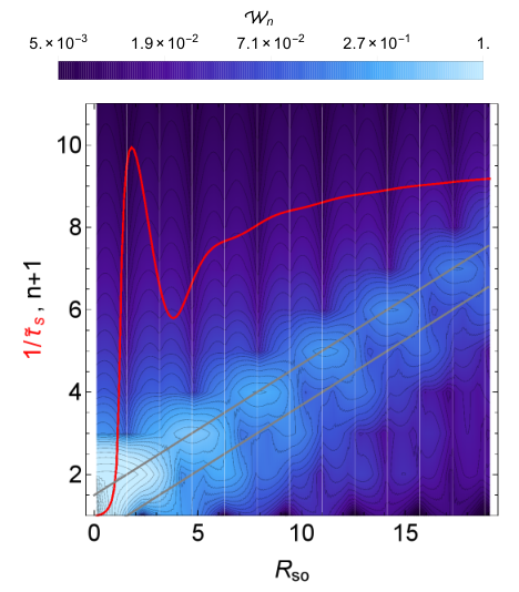
In Fig. 4, we display the numerically computed total spin relaxation rate $(1/\tau_{s})_{z}$ in terms of the 1D-diffusive rate $(1/\tau_{s})^{1D}_{z}$, Eq. (29), in dependence of $R_{\text{so}}$ and for different ratios of $Q_{\text{so}}^{2}/\delta_{\text{D}}^{(3)}$. The rate $(1/\tau_{s})_{z}$ is defined by the time, after which the z-component of the total spin is decayed to the factor $\mathcal{S}_{z}(t)/\mathcal{S}_{z}(0)=e^{-1}$ of its initial value. Notice that, here a single-exponential fit is not necessarily reliable for the extraction of the spin relaxation rate since a single-exponential decay is only given for an eigenstate. Most striking is the massive increase of the spin relaxation rate for small values of $R_{\text{so}}$. The peak in the relaxation rate occurs almost precisely at $R_{\text{so}}=\pi/2$. We can understand this behavior by noting that for $R_{\text{so}}=\pi/2$ the $\ket{1,\pm 1}$-components of $\mathbf{s}_{0}^{\prime}$ can be well represented by the basis functions $\braket{\mathbf{r}|n=1,l=\mp 1,0}$. The respective boundary-induced relaxation rate is given by $(1/\tau_{s})_{1,|1|}=D_{e}(2\zeta_{1,1}/\pi)^{2}Q_{\text{so}}^{2}$, which is remarkably of the order of magnitude of the bulk spin relaxation rate. Similar but less pronounced resonances occur at larger integer values of $R_{\text{so}}/(\pi/2)$. As the radius $R_{\text{so}}$ further increases, the influence of higher modes gains more and more weight and the mixing of the modes becomes larger, which is depicted in Fig. 5. Nevertheless, the total increment is weakened by the simultaneously decreasing significance of the boundary-induced relaxation rates, which scale with $\propto R_{\text{so}}^{-1}$. At last, we illustrate in Fig. 6 the dynamical evolution of a spin density for the radius $R_{\text{so}}=10$, where the corresponding (gauge-transformed) initial state $\mathbf{s}_{0}^{\prime}$ strongly deviates from a spatially homogeneous distribution. Similar characteristic behavior was observed in planar quantum wires.[26] The relaxation process of the local spin density $\mathbf{s}(\mathbf{r},t)$ is strongly inhomogeneous and locally accelerated due to the fast-decaying modes. As the optical measurement typically provides information about the average spin $\bm{\mathcal{S}}(t)$, the long-lived spin states are masked by the fast-decaying modes. Note, that also in 2D systems an accelerated decay can be found if the initial state is spatially not homogeneous.[80]

In conclusion, we found a dramatic change of the total average spin relaxation rate for an initially homogeneously $z$-polarized spin density with the wire radius. Within the range of ${0<R/L_{\text{so}}\leq 1/4}$ (with $l_{e}<R$) the spin relaxation rate varies from the very small 1D-diffusive rate to a rate which is of the order of the bulk spin relaxation rate. This peculiar feature should be directly detectable in optical spin injection measurements.[48] We stress that, this behavior cannot be observed in zinc-blende nanowires since the homogeneous initial state, Eq. (30), constitutes an eigenstate that is independent of the wire radius.[30] This is a consequence of the missing effective vector potential in Eq. (11) which in turn is due to the lack of first-degree spherical harmonic SOC terms, in particular, the $k$-linear contribution.

In order to emphasize the significance of the results, we provide a concrete example of a wurtzite InAs nanowire grown along the [0001]-axis. The spin relaxation in these systems has been experimentally investigated recently in Refs. 50, 49 by means of magnetoconductance measurements. Both studies use nanowires with diameters of about $80\text{\,}\mathrm{n}\mathrm{m}$ and carrier densities which correspond to a 3D electron density $n\sim${10}^{17}\text{\,}\mathrm{c}\mathrm{m}^{-3}$$. The authors extract values for the spin relaxation length from fitting using different theoretical models. Ref. 50 applies the model of Kettemann[27] developed for diffusive planar wires with DP spin relaxation. On the other hand, Ref. 49 uses the 1D magnetoconductance model of Kurdak et al.,[81] which is developed for ballistic planar wires. As already pointed out in Ref. 49, we emphasize that in both situations the utilized model does not include an accurate description of the wurtzite nanowire. Ref. 50 observes spin relaxation lengths of $75\text{\,}\mathrm{n}\mathrm{m}$ and $100\text{\,}\mathrm{n}\mathrm{m}$ for two different samples and a fixed gate voltage. In Ref. 49 various gating techniques are used which yield spin relaxation lengths of 150-$170\text{\,}\mathrm{n}\mathrm{m}$ for low gate voltages.

For comparison with our findings, we consider an average effective mass $m$ of the $\Gamma_{7}$ conduction band of wurtzite InAs as $m=(2m_{\perp}+m_{\parallel})/3$, where $m_{\parallel}=0.042\,m_{0}$, $m_{\perp}=0.037\,m_{0}$, and $m_{0}$ denotes the bare electron mass.[47, 46] The respective SOC coefficients read as $\gamma_{\text{R}}^{\text{int}}=$0.3\text{\,}\mathrm{e}\mathrm{V}\AA$$, $\gamma_{\text{D}}=$132.5\text{\,}\mathrm{e}\mathrm{V}\AA^{3}$$, and $b=-1.24$.[45] The Fermi wave vector $k_{F}$ can be estimated from the 3D electron density $n$ as $k_{F}=(3\pi^{2}n)^{1/3}$. The DP spin relaxation length is related to the spin lifetime $\tau_{s}$ as $l_{s}=\sqrt{D_{e}\tau_{s}}$. Let us concentrate on the relaxation of spin states that are homogeneously polarized in real space since the bulk eigenstates coincide with the nanowire eigenstates in the 1D-diffusive limit. In Fig. 7, we compare the spin precession length and the spin relaxation lengths of the bulk and the long-lived spin states in the 1D diffusive limit with the spin relaxation rates Eqs. (17) and (29), respectively. In general, the density-modulation enters through the parameters $\delta_{\text{D}}^{(1)}$ and $\delta_{\text{D}}^{(3)}$, which result from the $k$-cubic SOC terms. Remarkably, the spin precession length, i.e., $L_{\text{so}}=\pi\hbar^{2}/[m(\gamma_{\text{R}}^{\text{int}}+\delta_{\text{D}}^{(1)})]$, diverges for a large density of $n=$3.4\text{\times}{10}^{18}\text{\,}\mathrm{c}\mathrm{m}^{-3}$$ since the coefficients $\delta_{\text{D}}^{(1)}$ and $\gamma_{\text{R}}$ cancel each other. In this case, the bulk spin relaxation lengths are solely determined by the $k$-cubic terms and, therefore, the relaxation lengths of bulk and long-lived spin states coincide.

Focusing on the regime of low to moderate electron densities, i.e., $n<${10}^{18}\text{\,}\mathrm{c}\mathrm{m}^{-3}$$, the spin precession length alters only insignificantly, i.e., $L_{\text{so}}=200-$350\text{\,}\mathrm{n}\mathrm{m}$$. Moreover, the spin relaxation lengths of the long-lived spin states ($>$1\text{\,}\mu\mathrm{m}$$) are at least two orders of magnitude larger than the bulk spin relaxation lengths ($<$60\text{\,}\mathrm{n}\mathrm{m}$$). As we have seen above, for nanowires with diameter $d>L_{\text{so}}/2=100-$175\text{\,}\mathrm{n}\mathrm{m}$$ the optical measurement will detect a spin relaxation length that is of the order of magnitude of the relaxation length in the bulk. This is in strong contrast to the magnetoconductance measurement, which probes the spin relaxation of the long-lived spin states and hardly changes with the radius (cf. Fig. 2). Hence, there is a large discrepancy between experimental characterization methods. These findings also indicate that in Refs. 49, 50 the obtained spin relaxation lengths predominantly result from the externally induced Rashba SOC, assuming that the results do not largely deviate due to the employed magnetoconductance model. This reasoning is also in agreement with the presumptions made in Ref. 50. Last, it should be mentioned that for InAs in the low-density range additional SOC effects due to Fermi level surface pinning may become relevant.[82, 58, 83] Their impact on the intrinsic spin relaxation in wurtzite nanowires shall be discussed elsewhere.

We conclude that it will be a delicate task to gain information about the intrinsic spin relaxation and the SOC coefficients from both experimental techniques. In magnetoconductance measurements owing to the long-lived spin states the intrinsic relaxation features can be easily covered by the externally induced Rashba terms due to electrical gating. On the other hand, in optical spin orientation the long-lived spin states are only excited in the 1D diffusive limit, where $R/L_{\text{so}}\ll 1$. Beyond this regime, the measured lifetime corresponds to a superposition of states and can strongly differ from the one of the long-lived spin states.

For small external fields, i.e., $Q_{\text{so}}^{\prime}/Q_{\text{so}}\ll 1$, the term in $\kappa$, which couples to the wave vector $Q_{z}$ can be neglected and the global minimum of the spectrum is found at $Q_{z}=0$. In this case, the triplet eigenvalues $E^{(0)}_{T,\pm}$ simplify to gaped unit parabolas, i.e.,

to second order in $R_{\text{so}}(R_{\text{so}}^{\prime})$.

In analogy and for better comparison to many other previous works,[84, 77, 27, 58, 30] the spin relaxation time is defined here by the global minimum of the spectrum at $Q_{z}=0$, which describes the decay of a spin density, that is homogeneously excited along the wire axis. Even though it is determined by the relative strength of the extrinsic and intrinsic SOC, in the limit $R_{\text{so}}\rightarrow 0$ and $R_{\text{so}}^{\prime}\rightarrow 0$ the lowest eigenvalue is always given by $E^{(0)}_{T,0}(0)$. Therefore, we define here

The eigenvectors of $\hat{H}_{c}$, that correspond to the eigenvalues $E^{(0)}_{T,j}(0)$ are $\mathbf{b}_{0}={}\mathbf{\hat{x}},\mathbf{b}_{-}={}\mathbf{\hat{y}},$ and $\mathbf{b}_{+}={}\mathbf{\hat{z}}$ in the basis of spin density components to lowest order in $Q_{\text{so}}\rho$ ($Q_{\text{so}}^{\prime}\rho$).

In our previous work,[30] we have seen that for zinc-blende wires a dominating external field was necessary to observe WAL characteristics. The latter are urgent for an unambigious parameter fitting. For $\eta<1$, the minimum of $E^{(0)}_{T,-}$ moves to finite wave vectors

to second order in $R_{\text{so}}(R_{\text{so}}^{\prime})$, which yields the gap

to second order in $R_{\text{so}}(R_{\text{so}}^{\prime})$. Using this, we can rewrite the eigenvalues $E^{(0)}_{T,\pm}$ as

For large extrinsic SOC, the gap $E^{(0)}_{T,-}(|Q_{z,0}|)$ turns into the global minimum of the spectrum, which underlines again the superiority of helical spin states and was also seen in other systems.[27, 26, 28, 29, 58, 16, 30] Neglecting the term $\propto\eta^{2}$, we can estimate the transition to occur at

for $R_{\text{so}}\wedge R_{\text{so}}^{\prime}\leq 1$. Note that for $\eta\ll 1$, the gap is about half as large as the global minimum for $Q_{z}=0$, i.e., $E^{(0)}_{T,0}(0)$.

References

- [1] P. Yang, R. Yan, and M. Fardy, Nano Lett. 10, 1529 (2010).
- [2] V. Mourik, K. Zuo, S. M. Frolov, S. R. Plissard, E. P. A. M. Bakkers, and L. P. Kouwenhoven, Science 336, 1003 (2012).
- [3] A. Das, Y. Ronen, Y. Most, Y. Oreg, M. Heiblum, and H. Shtrikman, Nat. Phys. 8, 887 (2012).
- [4] L. Hofstetter, S. Csonka, J. Nygård, and C. Schönenberger, Nature 461, 960 (2009).
- [5] J. A. van Dam, Y. V. Nazarov, E. P. A. M. Bakkers, S. De Franceschi, and L. P. Kouwenhoven, Nature 442, 667 (2006).
- [6] S. Heedt, I. Wehrmann, K. Weis, R. Calarco, H. Hardtdegen, D. Grützmacher, Th. Schäpers, C. Morgan, and D. E. Bürgler, “Toward spin electronic devices based on semiconductor nanowires,” in Future Trends in Microelectronics (John Wiley & Sons, Inc., 2013) pp. 328–339.
- [7] A. B. Greytak, C. J. Barrelet, Y. Li, and C. M. Lieber, Appl. Phys. Lett. 87, 151103 (2005).
- [8] J. Xiang, W. Lu, Y. Hu, Y. Wu, H. Yan, and C. M. Lieber, Nature 441, 489 (2006).
- [9] S. Nadj-Perge, S. M. Frolov, E. P. A. M. Bakkers, and L. P. Kouwenhoven, Nature 468, 1084 (2010).
- [10] S. Nadj-Perge, V. S. Pribiag, J. W. G. van den Berg, K. Zuo, S. R. Plissard, E. P. A. M. Bakkers, S. M. Frolov, and L. P. Kouwenhoven, Phys. Rev. Lett. 108, 166801 (2012).
- [11] P. Krogstrup, H. I. Jørgensen, M. Heiss, O. Demichel, J. V. Holm, M. Aagesen, J. Nygård, and A. Fontcuberta i Morral, Nat. Photonics 7, 306 (2013).
- [12] X. Dai, S. Zhang, Z. Wang, G. Adamo, H. Liu, Y. Huang, C. Couteau, and C. Soci, Nano Lett. 14, 2688 (2014).
- [13] P. E. Faria Junior, G. Xu, J. Lee, N. C. Gerhardt, G. M. Sipahi, and I. Žutić, Phys. Rev. B 92, 075311 (2015).
- [14] X. Dai, A. Messanvi, H. Zhang, C. Durand, J. Eymery, C. Bougerol, F. H. Julien, and M. Tchernycheva, Nano Lett. 15, 6958 (2015).
- [15] M. I. D’yakonov and V. I. Perel’, Sov. Phys. Solid State 13, 3023 (1972), [Fiz. Tverd. Tela 13, 3581 (1971)].
- [16] M. Kammermeier, P. Wenk, and J. Schliemann, Phys. Rev. Lett. 117, 236801 (2016a).
- [17] P. Wenk, M. Kammermeier, and J. Schliemann, Phys. Rev. B 93, 115312 (2016).
- [18] J. Schliemann, J. C. Egues, and D. Loss, Phys. Rev. Lett. 90, 146801 (2003).
- [19] B. A. Bernevig, J. Orenstein, and S.-C. Zhang, Phys. Rev. Lett. 97, 236601 (2006).
- [20] M. Trushin and J. Schliemann, New J. Phys. 9, 346 (2007).
- [21] T. Dollinger, M. Kammermeier, A. Scholz, P. Wenk, J. Schliemann, K. Richter, and R. Winkler, Phys. Rev. B 90, 115306 (2014).
- [22] J. Schliemann, Rev. Mod. Phys. 89, 011001 (2017).
- [23] M. Kohda and G. Salis, Semicond. Sci. Technol. 32, 073002 (2017).
- [24] A. G. Mal’shukov and K. A. Chao, Phys. Rev. B 61, R2413 (2000).
- [25] A. A. Kiselev and K. W. Kim, Phys. Rev. B 61, 13115 (2000).
- [26] P. Schwab, M. Dzierzawa, C. Gorini, and R. Raimondi, Phys. Rev. B 74, 155316 (2006).
- [27] S. Kettemann, Phys. Rev. Lett. 98, 176808 (2007).
- [28] P. Wenk and S. Kettemann, Phys. Rev. B 81, 125309 (2010a).
- [29] P. Wenk and S. Kettemann, Phys. Rev. B 83, 115301 (2011).
- [30] M. Kammermeier, P. Wenk, J. Schliemann, S. Heedt, Th. Gerster, and Th. Schäpers, Phys. Rev. B 96, 235302 (2017).
- [31] Th. Schäpers, V. A. Guzenko, M. G. Pala, U. Zülicke, M. Governale, J. Knobbe, and H. Hardtdegen, Phys. Rev. B 74, 081301 (2006).
- [32] A. W. Holleitner, V. Sih, R. C. Myers, A. C. Gossard, and D. D. Awschalom, New J. Phys. 9, 342 (2007).
- [33] F. Glas, J.-C. Harmand, and G. Patriarche, Phys. Rev. Lett. 99, 146101 (2007).
- [34] G. Patriarche, F. Glas, M. Tchernycheva, C. Sartel, L. Largeau, J.-C. Harmand, and G. E. Cirlin, Nano Lett. 8, 1638 (2008).
- [35] L. Zhang, J.-W. Luo, A. Zunger, N. Akopian, V. Zwiller, and J.-C. Harmand, Nano Lett. 10, 4055 (2010).
- [36] P. Krogstrup, S. Curiotto, E. Johnson, M. Aagesen, J. Nygård, and D. Chatain, Phys. Rev. Lett. 106, 125505 (2011).
- [37] T. Rieger, M. I. Lepsa, Th. Schäpers, and D. Grützmacher, J. Cryst. Growth 378, 506 (2013).
- [38] P. Schroth, M. Köhl, J.-W. Hornung, E. Dimakis, C. Somaschini, L. Geelhaar, A. Biermanns, S. Bauer, S. Lazarev, U. Pietsch, and T. Baumbach, Phys. Rev. Lett. 114, 055504 (2015).
- [39] A. Fontcuberta i Morral, Nature 531, 308 (2016).
- [40] D. Jacobsson, F. Panciera, J. Tersoff, M. C. Reuter, S. Lehmann, S. Hofmann, K. A. Dick, and F. M. Ross, Nature 531, 317 (2016).
- [41] Y. Zhang, Z. Sun, A. M. Sanchez, M. Ramsteiner, M. Aagesen, J. Wu, D. Kim, P. Jurczak, S. Huo, L. J. Lauhon, and H. Liu, Nano Letters 18, 81 (2018).
- [42] A. De and C. E. Pryor, Phys. Rev. B 81, 155210 (2010).
- [43] T. Cheiwchanchamnangij and W. R. L. Lambrecht, Phys. Rev. B 84, 035203 (2011).
- [44] G. A. Intronati, P. I. Tamborenea, D. Weinmann, and R. A. Jalabert, Phys. Rev. B 88, 045303 (2013).
- [45] M. Gmitra and J. Fabian, Phys. Rev. B 94, 165202 (2016).
- [46] T. Campos, P. E. Faria Junior, M. Gmitra, G. M. Sipahi, and J. Fabian, Phys. Rev. B 97, 245402 (2018).
- [47] P. E. Faria Junior, T. Campos, C. M. O. Bastos, M. Gmitra, J. Fabian, and G. M. Sipahi, Phys. Rev. B 93, 235204 (2016).
- [48] S. Furthmeier, F. Dirnberger, M. Gmitra, A. Bayer, M. Forsch, J. Hubmann, C. Schüller, E. Reiger, J. Fabian, T. Korn, and D. Bougeard, Nat. Commun. 7, 12413 (2016).
- [49] Z. Scherübl, G. Fülöp, M. H. Madsen, J. Nygård, and S. Csonka, Phys. Rev. B 94, 035444 (2016).
- [50] T. S. Jespersen, P. Krogstrup, A. M. Lunde, R. Tanta, T. Kanne, E. Johnson, and J. Nygård, Phys. Rev. B 97, 041303 (2018).
- [51] A. E. Hansen, M. T. Björk, I. C. Fasth, C. Thelander, and L. Samuelson, Phys. Rev. B 71, 205328 (2005).
- [52] S. Dhara, H. S. Solanki, V. Singh, A. Narayanan, P. Chaudhari, M. Gokhale, A. Bhattacharya, and M. M. Deshmukh, Phys. Rev. B 79, 121311 (2009).
- [53] X.-J. Hao, T. Tu, G. Cao, C. Zhou, H.-O. Li, G.-C. Guo, W. Y. Fung, Z. Ji, G.-P. Guo, and W. Lu, Nano Lett. 10, 2956 (2010).
- [54] I. van Weperen, B. Tarasinski, D. Eeltink, V. S. Pribiag, S. R. Plissard, E. P. A. M. Bakkers, L. P. Kouwenhoven, and M. Wimmer, Phys. Rev. B 91, 201413 (2015).
- [55] P. Roulleau, T. Choi, S. Riedi, T. Heinzel, I. Shorubalko, T. Ihn, and K. Ensslin, Phys. Rev. B 81, 155449 (2010).
- [56] D. Liang and X. P. Gao, Nano Lett. 12, 3263 (2012).
- [57] K. Takase, Y. Ashikawa, G. Zhang, K. Tateno, and S. Sasaki, Sci. Rep. 7, 930 (2017).
- [58] M. Kammermeier, P. Wenk, J. Schliemann, S. Heedt, and Th. Schäpers, Phys. Rev. B 93, 205306 (2016b).
- [59] S. G. Carter, Z. Chen, and S. T. Cundiff, Phys. Rev. Lett. 97, 136602 (2006).
- [60] J. D. Koralek, C. P. Weber, J. Orenstein, B. A. Bernevig, S.-C. Zhang, S. Mack, and D. D. Awschalom, Nature 458, 610 (2009).
- [61] G. Wang, B. L. Liu, A. Balocchi, P. Renucci, C. R. Zhu, T. Amand, C. Fontaine, and X. Marie, Nat. Commun. 4, 2372 (2013).
- [62] J. H. Buß, J. Rudolph, S. Starosielec, A. Schaefer, F. Semond, Y. Cordier, A. D. Wieck, and D. Hägele, Phys. Rev. B 84, 153202 (2011).
- [63] S. Jahangir, F. Doğan, H. Kum, A. Manchon, and P. Bhattacharya, Phys. Rev. B 86, 035315 (2012).
- [64] W. Stefanowicz, R. Adhikari, T. Andrearczyk, B. Faina, M. Sawicki, J. A. Majewski, T. Dietl, and A. Bonanni, Phys. Rev. B 89, 205201 (2014).
- [65] I. Zutic, J. Fabian, and S. Das Sarma, Rev. Mod. Phys. 76, 323 (2004).
- [66] M. Wu, J. Jiang, and M. Weng, Phys. Rep. 493, 61 (2010).
- [67] S. Hikami, A. I. Larkin, and Y. Nagaoka, Prog. Theor. Phys. 63, 707 (1980).
- [68] P. Wenk and S. Kettemann, in Handbook on Nanophysics, edited by K. Sattler (Francis & Taylor, 2010) p. 49.
- [69] L. E. Golub, Phys. Rev. B 71, 235310 (2005).
- [70] M. M. Glazov and L. E. Golub, Semicond. Sci. Tech. 24, 064007 (2009).
- [71] Y. Araki, G. Khalsa, and A. H. MacDonald, Phys. Rev. B 90, 125309 (2014).
- [72] B. L. Al’tshuler and A. G. Aronov, JETP Lett. 33, 499 (1981), [Pis’ma Zh. Eskp. Teor. Fiz. 33, No. 10, 515 (1981)].
- [73] I. L. Aleiner and V. I. Fal’ko, Phys. Rev. Lett. 87, 256801 (2001).
- [74] J. S. Meyer, V. I. Fal’ko, and B. L. Altshuler, in Nato Science Series II, Vol. 72, edited by I. V. Lerner, B. L. Altshuler, V. I. Fal’ko, and T. Giamarchi (Kluwer Academic Publishers, Dordrecht, 2002) p. 117.
- [75] P. E. Faria Junior, G. Xu, Y.-F. Chen, G. M. Sipahi, and I. Žutić, Phys. Rev. B 95, 115301 (2017).
- [76] Y. V. Pershin and V. A. Slipko, Phys. Rev. B 82, 125325 (2010).
- [77] W. Knap, C. Skierbiszewski, A. Zduniak, E. Litwin-Staszewska, D. Bertho, F. Kobbi, J. L. Robert, G. E. Pikus, F. G. Pikus, S. V. Iordanskii, V. Mosser, K. Zekentes, and Yu. B. Lyanda-Geller, Phys. Rev. B 53, 3912 (1996).
- [78] P. Wenk, Itinerant Spin Dynamics in Structures of Reduced Dimensionality, Ph.D. thesis, Jacobs University Bremen (2011).
- [79] M. O. Hachiya, G. Usaj, and J. C. Egues, Phys. Rev. B 89, 125310 (2014).
- [80] V. A. Froltsov, Phys. Rev. B 64, 045311 (2001).
- [81] Ç. Kurdak, A. M. Chang, A. Chin, and T. Y. Chang, Phys. Rev. B 46, 6846 (1992).
- [82] A. Bringer and Th. Schäpers, Phys. Rev. B 83, 115305 (2011).
- [83] V. E. Degtyarev, S. V. Khazanova, and N. V. Demarina, Sci. Rep. 7, 3411 (2017).
- [84] S. V. Iordanskii, Yu. B. Lyanda-Geller, and G. E. Pikus, JETP Lett. 60, 206 (1994), [Pis’ma Zh. Eksp. Teor. Fiz. 60, 199 (1994)].
- [85] B. L. Altshuler and A. G. Aronov, Solid State Communications 38, 11 (1981).
- [86] J. M. Kikkawa and D. D. Awschalom, Phys. Rev. Lett. 80, 4313 (1998).
- [87] R. I. Dzhioev, K. V. Kavokin, V. L. Korenev, M. V. Lazarev, B. Y. Meltser, M. N. Stepanova, B. P. Zakharchenya, D. Gammon, and D. S. Katzer, Phys. Rev. B 66, 245204 (2002).