Non-Hermitian coherent states for finite-dimensional systems
Abstract
We introduce Gilmore-Perelomov coherent states for non-unitary representations of non-compact groups, and discuss the main similarities and differences with respect to ordinary unitary Gilmore-Perelomov coherent states. The example of coherent states for the non-unitary finite dimensional representations of is considered and they are used to describe the propagation of light in coupled PT-symmetric optical devices.
1 Deparment of Mathematics, Experimental Sciences Faculty,
Campus las Lagunillas, University of Jaén, 23071 Jaén, Spain.
JulioGuerrero@ujaen.es
2 Computer Science Faculty, Campus de Espinardo, University of Murcia, 30100 Murcia, Spain.
1 Introduction and physical motivation
Non-hermitian Hamiltonians have been used for a long time as effective Hamiltonians (think, for instance, of the optical potential in nuclear physics [1]). With the introduction of -symmetric Hamiltonians [2] in Quantum Mechanics they became very popular, however only a few papers have been devoted to coherent states (CS) for non-Hermitian systems (see [3], where Gazeau-Klauder CS are constructed using the definition of scalar product in terms of the CPT norm, [4, 5, 6, 7, 8, 9] where the notion of pseudo-bosons and bi-coherent states are introduced, or [10, 11]) as compared with the huge amount of papers devoted to usual coherent states.
Non-hermitian systems, in particular PT-symmetric ones, have found the goose that laid the golden eggs in optics, in particular in discrete photonic systems (DPS), where the first experimental11 1 The first theoretical proposal of -symmetry in optics was given in [12]. realization of PT-symmetry was realized [13].
Let us describe briefly DPS and later we shall study the implications on non-hermiticity on these systems.
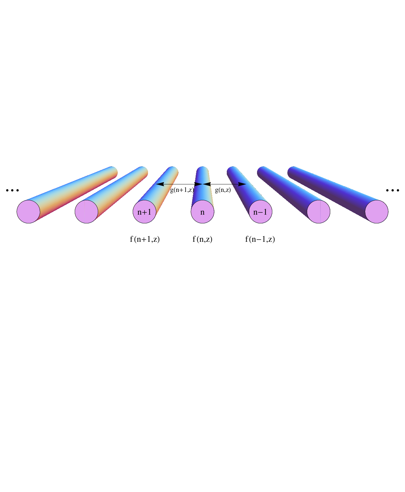
Consider an (infinite) planar array of optical waveguides, like the one of Fig. 1. Using Maxwell theory of electromagnetism, and performing some approximations (valid in a wide range of applications in DPS), we arrive to a set of coupled first-order differential equations describing the scalar magnitude of the (either electric o magnetic) field inside the waveguides (see for instance, [14]):
| (1) |
where we have supposed that the couplings between adjacent waveguides (with units inverse of length) and the propagation constant (proportional to the refractive index and also with units inverse of length) depend both on the waveguide number and the distance along the waveguide [15].
Note that if the coupling vanishes for one value of (for all ) the array can be semiinfinite. If it vanishes for two or more values of the array can be finite.
Writing eq. (1) in matrix form and using Dirac’s bra-ket notation we see that this set of equations can be written in Schrödinger-like form (equivalence is established by simply changing ):
| (2) |
where
| (3) |
and
The Hamiltonian reads:
| (4) |
where is the number operator, and and are the step-down and step-up operators, respectively.
1.1 Symmetric DPS
The differential equation
| (5) |
can be solved by group-theoretical methods (like Wei-Norman factorization [16]) if
| (6) |
with constant matrices realizing a representation of a Lie algebra (associated with the Lie group ) with . In this case the propagator (evolution operator in the case of Schrödinger equation) can be explicitly computed:
| (7) |
where is the initial value of and the functions satisfy non-linear first-order coupled differential equations (in ) involving the structure constants and the coefficients . Here represents an element of the group that, for fixed , describes a curve in , and is a representation of (the one obtained by exponentiation of the representation of defined by the matrices ).
Note that the propagator satisfies the composition property
| (8) |
(i.e. defining a groupoid), and if the Hamiltonian does not depend on , then and the composition property becomes the usual homomorphysm property
| (9) |
In this case the curve constitutes a one-parameter subgroup of generated by the Lie algebra element . Let’s denote this subgroup by .
Define as the family of Gilmore-Perelomov coherent states [17] associated with the group , the representation , and the fiducial vector . Then is a one-parameter subfamily of coherent states. If does not depend on , then the subfamily is by itself a family of coherent states associated with the subgroup , the representation restricted to , and the fiducial vector .
An interesting fact is that, since the Hamiltonian is always an element of the Lie algebra , we have temporal (or rather, spatial) stability [18], since the propagation along always remains in the family (i.e. for some ). If further does not depend on and it is a compact operator, there will be periodic revivals, i.e. the system returns to the original state after multiples of some length , and in general .
Strictly speaking, for to be a coherent state it is required that the representation be unitary and square-integrable (modulo a subgroup, perhaps [19]), and the fiducial vector be admissible. However, in the examples we are considering (and in the general discussion we provide later in Sec. 2), we shall drop the requirement of unitarity, but keeping square-integrability, and see how this still provides a well defined notion of coherent states.
We shall focus on finite DPS, i.e. the index set will be finite. If is a compact group (like SU(2)), is unitary and the total light power is conserved along propagation. If is a non-compact group (like or ), is not unitary and the total power is not conserved. Non-unitarity is caused by non-Hermiticity of the Hamiltonian.
Non-Hermitian Hamiltonians describe DPS with losses and/or gain, or non-symmetrical couplings (due, for instance, to torsion of non-identical waveguides or in effective Hamiltonians for some non-linear DPS [20]).
1.2 Non-Hermitian dimer
Let us focus on a finite DPS with two waveguides, usually known as dimer. Consider the most general non-Hermitian coupling matrix
| (10) |
Setting the propagation constants relative to their average,
| (11) |
gives the traceless effective non-Hermitian coupling matrix,
| (12) |
and the differential system,
| (13) |
Note that the Hamiltonian is an element of the Lie algebra, where , with basis , being the standard angular momentum operators (Pauli matrices in the case of the dimer). More precisely, it can be written as:
| (14) | |||||
Designing appropriately the parameters in the Hamiltonian some of the coefficients in the right hand side of previous equation can vanish and thus will be an element of the Lie subalgebra , whose generators are denoted by . For this purpose, there are various possibilities:
| (15) |
Experimentally, it is easier to realize a Hamiltonian that can be written as a combination of , imposing , and (i.e. , real and pure imaginary). If we further impose , i.e. and real (i.e. real and symmetrical couplings), this system corresponds to a PT-symmetric DPS with balanced gain/loss [21, 22]. In the next subsection a realization of this case is discussed in detail.
1.3 Finite DPS with symmetry: PT-symmetric DPS
The Hamiltonian for a finite DPS with underlying symmetry can be taken as
| (16) |
If we take a unitary representation of with spin , we obtain a non-unitary representation of with “spin” . Since this representation is finite dimensional with dimension , our system will have waveguides.
Under the transformation () and “” transformation (, ) the Hamiltonian changes to:
| (17) |
provided and are even. Therefore the system is -symmetric.
However, for some values of the parameters, the -symmetry can be spontaneously broken, in the sense that wavefunctions are not PT-symmetric.
For the case and , simple analytical expressions can be obtained. Three cases have to be considered, depending on whether is positive, zero or pure imaginary, corresponding to three qualitatively different propagations: periodic (but with total power not conserved along propagation, unbroken PT-symmetry), growing with a power law, or growing with an exponential law, respectively (broken PT-symmetry). See Fig. 2 showing the light intensities for a PT-symmetric DPS with three waveguides.
Guided by the physical motivation of non-hermitian DPS, we shall try to provide in the rest of the paper a mathematical framework that describes the propagation of light in these devices as non-hermitian (or non-unitary) Gilmore-Perelomov coherent states.
2 Non-Hermitian Coherent States
As we have seen in the physical example, in some situations one has to handle systems possessing a symmetry group that it is realized through a non-unitary representation. To mathematically describe this situation, one has to resort (in the infinite dimensional case) to a more general setting than Hilbert spaces, and this is the notion of Banach space. However, to simulate some of the properties of unitary representations on Hilbert spaces, a “dual” representation is needed. Let us introduce the notion of contragredient representation associated to a non-unitary representation , following [23].
Let be a representation of a locally compact Lie group with Lie algebra in a reflexive22 2 We shall restrict to reflexive Banach spaces since in this case the formulation is simpler and more similar to the Hilbert space case, see [23]. Banach space :
| (18) |
Define the contragredient representation on the dual space , as .
Note that, since is assumed to be reflexive, we have that if is bounded and continuous, then is continuous, and that is irreducible if and only if is irreducible.
By definition, the pair verifies
| (19) |
where denotes the usual pairing between and .
Note that if is unitary (and is a Hilbert space, where is the scalar product, related to the pairing by Riesz representation theorem) then . In this sense, the pair generalizes the unitary case to the non-unitary case, in the more general setting of Banach spaces.
The notion of square integrability of a representation should be adapted to this more general setting as follows:
Definition 1
([23]) A representation on a reflexive Banach space is square integrable if there exist a non-zero vector (called admissible) such that
| (20) |
where is the (left) Haar measure on .
An analogous definition can be given for the contragredient representation:
Definition 2
([23]) The contragredient representation on is ∗-square integrable if there exist a non-zero vector (called ∗-admissible) such that
| (21) |
where is the (left) Haar measure on .
The set of admissible (resp. ∗-admissible) vectors is invariant under (resp. ).
From now on we shall say, to simplify the notation, that the representation is square integrable if it is ∗-square integrable and that the non-zero vector is admissible if it is ∗-admissible.
2.1 Non-hermitian Gilmore-Perelomov Coherent States
Definition 3
Given a square integrable representation on a reflexive Banach space and an admissible vector , a family of non-hermitian Gilmore-Perelomov Coherent States is given by:
| (22) |
The analogous “dual” definition is:
Definition 4
Given the square integrable representation on and an admissible vector , the dual family of non-hermitian Gilmore-Perelomov Coherent States is given by:
| (23) |
The idea of defining two families of coherent states can be seen as a generalization (in the sense of Gilmore-Perelomov coherent states) of bi-coherent states for the standard bosonic operators [4, 5, 6, 7, 8, 9].
The notion of square integrability (and its dual) is required to make sense of the following concepts (to avoid cluttering of notation we shall omit the dependence on the representation and the admissible vector on and ).
Definition 5
([23]) Let be a square integrable representation of the locally compact group on the reflexive Banach space , and an admissible vector for . Then the sampling (or analysis) operator is given by
| (24) |
The adjoint defines the synthesis operator:
| (25) |
There is an analogous definition for the dual case:
Definition 6
([23]) Let be a square integrable representation of the locally compact group on , and an admissible vector for . Then the dual sampling (or analysis) operator is given by
| (26) |
The adjoint defines the synthesis operator:
| (27) |
Let us introduce the Resolution operator :
| (28) |
and its dual .
A non-unitary version of Schur’s lemma can be stated. For this purpose, denote by the Banach algebra of bounded linear operators on the Banach space . We need the following results, that can be obtained by a slight modification of those in [24] (Corollary 3.2.9 and Theorem 4.2.2).
Lemma 1
Let be a bounded and irreducible representation of the Lie group on the Banach space . If we define , then is isomorphic to .
With this Lemma we can prove:
Proposition 1
Let be a reflexive Banach space. If is continuous and irreducible, the resolution operators and , if non-zero and bounded, are proportional to the identity operator on and , respectively.
Proof: Using the definitions of and and the invariance of the left Haar measure on , it is easy to check that
| (29) |
Thus and (defined analogously for ). Since is irreducible also is and by the previous Lemma both and are isomorphic to , and therefore and are proportional to the identity operators.
It should be stressed that the requirement that (and thus ) be bounded is crucial for the validity of the previous results (otherwise and it cannot be granted that is bounded). Also, the requirement of irreducibility is necessary to have that is bijective (and not just that is injective with having dense domain in .
If are square-integrable (with their respective admissible vectors), then we have that and are bounded (see [23]), and therefore Proposition 1 applies.
Similarly to the unitary case, a reproducing (or overlapping) kernel can be defined.
Definition 7
Let be a reflexive Banach space and a continuous representation of a Lie group on , with its contragredient representation. Define the Overlapping Kernel as:
| (30) |
Proposition 2
The overlapping kernel depends only on .
Proof:
| (31) |
where is the identity element in .
Proposition 2 means that is the kernel of a convolution operator on when is square integrable.
The overlapping kernel, in the unitary and square-integrable case, endorses the Hilbert subspace with a reproducing kernel Hilbert space structure, with kernel , which is square-integrable, hermitian () and positive definite. In the non-unitary case, if are square-integrable, we still have that the overlapping kernel is square-integrable, but since , we need two admissible functions and therefore and in general are not related to each other and does not make sense to speak about hermiticity and positive definiteness. Therefore, does not endorses with a reproducing kernel Hilbert space structure.
2.2 The non-square integrable case
If the representations are not square integrable, previous expressions are purely formal in the sense that the norm of and can be unbounded on (implying unbounded and non-integrable) due to the non-unitarity of and non-compactness of .
This means that, although it is possible to define a family of coherent states, it is useless in the sense that we cannot use it as a “basis”, and in particular it is not possible to reconstruct a function from its coefficients in this “basis”. This process requires the inverse of the resolution operator and this operator is not bounded (and even can be “infinite” in the sense that the integral on defining it is divergent).
Despite of these problems related to the lack of square-integrability, non-hermitian Coherent States can be physically meaningful in some situations, as shown in previous sections.
The reason can be understood as follows. Suppose is a non-compact Lie group and a non-unitary representation, with its contragredient representation. Suppose they are not square integrable and consider the maximal compact subgroup of . Since is compact, the restriction of the representations are both equivalent to a unitary representation of . Redefine such that restricted to coincide with . Since is compact is square-integrable, thus consider admissible vectors in and , respectively. The resolution operator is
| (32) |
where is a left-invariant Haar measure on and . is bounded and satisfy the interwinning property, Eq. (29), with respect to . In general is not irreducible (even if is) and therefore we cannot apply Prop. 1 to conclude that is proportional to the identity operator on (the same applies to on ).
Consider now and define the elliptic subgroups , where is a representative for a class . Define as the restriction to of . Then we have that the representations are square integrable and the resolution operator is given by: .
As before, in general are not irreducible (even if is) and therefore we cannot apply Prop. 1 to conclude that is proportional to the identity operator on .
These considerations can even be extended to the general case. Let be a non-unitary representation of the non-compact group on the Banach space . If is square integrable, then is topologically isomorphic to a Hilbert space and are equivalent to a unitary representation on (see [23], Theorem 3.13). This result can be seen as a group-theoretical version of the concept of pseudo-hermiticity (see [25]).
In the next section, motivated by the -symmetric dimer, we consider the example of the non-unitary finite-dimensional representations of , and discuss various ways of tackling the lack of square-integrability of the representations.
3 Example: SU(1,1) Non-hermitian coherent states
Consider the realization (see [17]) of . Note that this is a different realization to that of the -symmetric dimer, we shall use this one in this example since the compact generator of is , the usual convention in mathematics. All results discussed here apply to the case of the -symmetric dimer by changing
| (33) |
Thus, if we take the -dimensional unitary irreducible representation of , we get a -dimensional non-unitary irreducible representation of .
We shall use the following parametrization of the group elements (for the case , leading to the fundamental o defining representation, for other values of provides the different non-unitary representations of the group):
| (34) |
where (the unit disk in the complex plane), and . Note that are not the adjoint of each other, but instead . For this reason is not a unitary operator, in fact it is hermitian positive-definite. Thus eq. (34) provides explicitly the polar decomposition of the representation, and shows that it is non-unitary.
For instance, the case is:
| (35) |
The contragredient representation for this case is:
| (36) |
It is important to mention that, for general , matrix elements of both representations diverge as when . This is also the behavior of the largest eigenvalue.
Let us choose as fiducial vectors (other choices lead to similar results in this case) . Then the coherent states are:
The resolution operator is:
| (39) |
where is the left-invariant Haar measure on the group. The dual version is simply the adjoint. is divergent since the representation is not square integrable. The reason is that the behavior for of the matrix elements of , for arbitrary , is , and together with the integration measure gives which is divergent when integrated on .
This should be compared with the unitary representations of the discrete series of , which are infinite-dimensional, and the behavior for of the matrix elements of the corresponding resolution operator is , where is the Bargmann index characterizing the representation. Together with the integration measure gives and this is convergent when integrated on if . Therefore, the representations of the discrete series are unitary and square-integrable for .
Note that all expressions can be derived from those of the discrete series simply performing the change , with and half-integer.
The overlapping kernel is given by:
| (40) |
In this case the overlapping kernel is hermitian and positive definite (since is isomorphic to and ), but it is not bounded on and therefore it is not square-integrable. In fact, as commented previously, it coincides with the overlapping kernel for the coherent states associated with the representation of the discrete series with Bargmann index .
To overcome these problems there are many alternatives, as suggested in Sec. 2. We shall discuss some of them in the following subsections.
3.1 Restriction to the maximal compact subgroup
If we restrict the representation to the maximal compact subgroup , a double cover of , we obtain a unitary, although reducible, representation of . It decomposes into (for general ) irreducible unitary characters, labeled by . This case coincides with that of a representation of restricted to . In a sense this case is trivial since it reduces to a well-known, unitary case.
Denote by the restriction of the resolution operator to the compact subgroup (as defined in eq. (32)). Since the representation restricted to is reducible, is not proportional to the identity, and even non-invertible, in general. In this case is invertible only if the component-wise product of the vectors and is a vector with all its components different from zero. If all the components of this vector are identical, then is proportional to the identity.
The overlapping kernel restricted to , , is square-integrable on . Since in this finite-dimensional case and are isomorphic, we can choose as before and therefore is positive definite and hermitian. Thus, is a reproducing kernel for the Hilbert subspace .
3.2 Restriction to a subgroup of elliptic elements
Consider now the non-trivial case of a subgroup of elliptic elements in of the form , with a representative element of the class [26]. Restricting the representation to leads to a non-unitary finite-dimensional representation of , and this corresponds (with the changes (33)) to taking the propagator associated with a Hamiltonian in eq. (16) that is a compact operator. For the case of constant parameters and , this corresponds to the case , see Fig. 2 (left). This propagator generates non-hermitian coherent states with bounded (but non constant) norm on .
The resolution operator is bounded and invertible for arbitrary nonzero vectors and (there are only a few values of , depending on the components of and for which it is non-invertible). For a given non-zero and a given , there is a unique non-zero (up to normalization) that makes the resolution operator proportional to the identity. The overlapping kernel is square-integrable on .
3.3 Restriction to subgroups of hyperbolic and parabolic elements
The restriction to subgroups of parabolic or hyperbolic elements [26] always leads to non-square integrable representations for any choices of nonzero and . The subgroup of parabolic elements correspond (with the changes (33)) to the case , see Fig. 2 (center), and subgroups of hyperbolic elements correspond to the case , see Fig. 2 (right).
In these last cases other strategies should be adopted to overcome non-square integrability, and this will be considered in the next subsection.
3.4 Restriction to compact subsets
The non square-integrability of the representation is caused by the integration on the non-compact subset . We can consider compact subsets of (times ) that avoid the non square-integrability. For instance, we can take the following subsets:
- a)
, with fixed. The integration in this case is over the compact subset .
- b)
, with . The integration in this case is over the compact subset .
- c)
with , , . The integration in this case is over times a sum in .
In all these cases the resolution operator for the corresponding subfamily of coherent states is bounded and proper choices of and can be made to render it invertible and even proportional to the identity. Case (c) is similar to the construction made in [29, 30, 31] where discrete (pseudo-) frames of coherent states were constructed for unitary representations of , and the Heisenberg-Weyl group, respectively.
In none of these cases the subset constitutes a subgroup of , not even an homogeneous space, i.e. of the form for some subgroup . Therefore some of the properties of Gilmore-Perelomov [17] coherent states or coherent states modulo a subgroup [19] are lost. In particular, the subfamily of coherent states associated with them does not contain all the states generated by the propagator for Hamiltonians with , although they contain them for finite propagation distances (chosing appropriately and in case (b), for instance).
In any case, if the subfamily of coherent states associated with a compact subset leads to an invertible resolution operator, they form an overcomplete family and any state of the system can be expressed in terms of them.
4 Conclusions and outlook
In this work coherent states associated with non-unitary representations of non-compact Lie groups have been introduced motivated by the behavior of certain DPS with non-hermitian Hamiltonians (in particular -symmetric DPS), and following the general theory outlined in [23]. We have called these families of coherent states “non-hermitian” rather than “non-unitary” since we focus in the physical motivation (non-hermitian systems with a symmetry Lie group) rather than the mathematical setting (non-unitary representation of the symmetry Lie group).
Although we discuss for completeness the general, infinite-dimensional case, which requires the use of Banach spaces (versus Hilbert spaces for the unitary case) to account for the maximum generality, we shall focus in the examples in finite-dimensional (infinite-dimensional examples will be considered elsewhere), non-unitary representations, where all the subtleties of Banach spaces do not appear. See [23] for infinite-dimensional examples with non-trivial Banach spaces ( and with ).
The main obstruction for constructing coherent states for non-unitary representations comes from the lack of square-integrability of the representation. Different approaches have been used to circumvent this problem in the example of considered in Sec. 3, the most interesting one being the restriction to certain subgroups (in particular elliptic subgroups), where the representation restricted to the subgroup is still non-unitary but it is square-integrable. This is related to the physically interesting case of a -symmetric waveguide array in the regime of unbroken -symmetry. Other possibilities have been discussed, like the restriction to certain compact subsets of .
References
- [1] Foldy L.L.& Walecka J.D.: On the theory of the optical potential. Ann. Phys. 54, 447-504 (1969)
- [2] Bender C. M. & Boettcher S. : Real spectra in non-Hermitian Hamiltonians having PT-symmetry. Phys. Rev. Lett. 80, 5243–5246 (1998)
- [3] Roy B. & Roy P.: Coherent states of non-Hermitian quantum systems. Physics Letters A 359 110–113 (2006)
- [4] Trifonov D. A.: Pseudo-Boson Coherent and Fock States, in Differential Geometry, Complex Analysis and Mathematical Physics, eds. K. Sekigawa et al. (W. Scientific 2009), pp. 241-250. arXiv:quant-ph/0902.3744
- [5] Bagarello F.: Pseudobosons, Riesz bases, and coherent states. J. Math. Phys. 51, 023531 (2010)
- [6] Bagarello F.: Pseudo-bosons and Riesz Bi-coherent States, in Geometric Methods in Physics, series Trends in Mathematics, pp 15-23 (2016). arXiv:1610.09317v1 [math-ph]
- [7] Bagarello F.: Intertwining operators for non-self-adjoint Hamiltonians and bicoherent states. J. Math. Phys. 57, 103501 (2016)
- [8] Bagarello F.: Deformed quons and bi-coherent states Proc. Roy. Soc. A, DOI: 10.1098/rspa.2017.0049
- [9] Bagarello F.: kq-representation for pseudo-bosons, and completeness of bi-coherent states. JMAA 450, 631-643 (2017)
- [10] Ali S.T., Roknizadeh R. & Tavassoly M. K.: Representations of coherent states in non-orthogonal bases. J. Phys. A: Math. Gen. 37 (2004) 4407–4422
- [11] Rosas-Ortiz O., Zelaya K.: Bi-Orthogonal Approach to Non-Hermitian Hamiltonians with the Oscillator Spectrum: Generalized Coherent States for Nonlinear Algebras. Ann. Phys. 388 (2018) 26–53
- [12] Ruschhaupt A., Delgado F. and Muga J.G.: Physical realization of PT-symmetric potential scattering in a planar slab waveguide. J. Phys. A 38, L171–L176 (2005)
- [13] Rüter C. E., Makris K. G., El-Ganainy R., Christodoulides D. N., & Kip D.: Observation of parity-time symmetry in optics. Nature Phys. 6, 192 – 195 (2010)
- [14] Hardy A., Streifer W.: Coupled mode theory of parallel waveguides. J. Lightwave Technol. LT-3, 1135-1146 (1985)
- [15] Villanueva Vergara L. & Rodríguez-Lara, B. M.: Gilmore-Perelomov symmetry based approach to photonic lattices. Opt. Express 23, 22836 (2015)
- [16] Wei J. & Norman E.: Lie algebraic solution of linear differential equations. J. Math. Phys. 4, 575–81 (1963).
- [17] Perelomov A.: Generalized Coherent States and Their Applications. Springer (1986)
- [18] Antoine J.-P., Gazeau J.-P., Monceau P., Klauder J.R. and Penson K.A.: Temporally stable coherent states for infinite well and Pöschl–Teller potentials. J. Math. Phys. 42, 2349 (2001)
- [19] Ali S. T., Antoine J. P. & Gazeau J. P.: Coherent States, Wavelets, and Their Generalizations. Springer (2014)
- [20] Zhong Q., Ahmed A., Dadap J.I. , Osgood JR, R.M. and El-Ganainy, R.: Parametric amplification in quasi-PT symmetric coupled waveguide structures, New J. Phys. 18, 125006 (2016)
- [21] Rodríguez-Lara B. M. & Guerrero J.: Optical finite representation of the Lorentz group. Opt. Lett. 40, 5419–5701 (2015)
- [22] Huerta Morales J. D., Guerrero J., López-Aguayo S. & Rodríguez-Lara B. M.: Revisiting the optical PT-symmetric dimer. Symmetry 8, 83 (24p) (2016)
- [23] Zimmermann G.: Coherent States from Nonunitary Representations. Topics in Multivariate Approximation and Interpolation, K. Jetter, M. Buhmann, W. Haussmann, R. Schaback, and J. Stöckler (eds.) Number 12 in Studies in Computational Mathematics Elsevier, Amsterdam 2006, pp. 291–339; Zimmermann G.: Coherent States from Nonunitary Representations. Habilitation’s thesis at Vienna University (2005)
- [24] Aupetit B.: A Primer on Spectral Theory. Springer-Verlag. New York (1991).
- [25] Mostafazadeh A.: Pseudo-Hermitian Representation of Quantum Mechanics. Int. J. Geom. Methods Mod. Phys. 07, 1191 (2010)
- [26] Simon B.: Orthogonal Polynomials on the Unit Circle. AMS Colloquium Publications, vol. 54, part 2, AMS, Provedence (2009)
- [27] Gordon R.: Harmonic oscillation in a spatially finite array waveguide. Opt. Lett. 29, 2752 (2004)
- [28] Perez-Leija, A. P. et al.: Coherent quantum transport in photonic lattices. Phys. Rev. A87, 012309-1–012309-8 (2013).
- [29] Calixto M., Guerrero J. & Sánchez-Monreal J. C.: Sampling Theorem and Discrete Fourier Transform on the Riemann Sphere. J. Fourier Anal. Appl. 14, 538–567(2008)
- [30] Calixto M., Guerrero J. & Sánchez-Monreal J. C.: Sampling Theorem and Discrete Fourier Transform on the Hyperboloid. J. Fourier Anal. Appl. 17 240–264 (2011)
- [31] Calixto M., Guerrero J. & Sánchez-Monreal J. C.: Almost complete coherent state subsystems and partial reconstruction of wavefunctions in the Fock-Bargmann phase-number representation. J. Phys. A 45, 244029 (2012)